Meta-learning Recommendation of Default Hyper-parameter Values ...

Meta-learning Recommendation of Default Hyper-parameter Values for SVMs in Classifications Tasks Rafael G. Mantovani1 , Andr´e L. D. Rossi2 , Joaquin Vanschoren3 , and Andr´e C. P. L. F. Carvalho1 1

3

Universidade de S˜ ao Paulo (USP), So Carlos - Brazil, {rgmantov,andre}@icmc.usp.br 2 Universidade Estadual Paulista (UNESP), Itapeva - SP, Brazil [email protected] Eindhoven University of Technology (TU/e), Eindhoven, The Netherlands [email protected]

Abstract. Machine learning algorithms have been investigated in several scenarios, one of them is the data classification. The predictive performance of the models induced by these algorithms is usually strongly affected by the values used for their hyper-parameters. Different approaches to define these values have been proposed, like the use of default values and optimization techniques. Although default values can result in models with good predictive performance, different implementations of the same machine learning algorithms use different default values, leading to models with clearly different predictive performance for the same dataset. Optimization techniques have been used to search for hyper-parameter values able to maximize the predictive performance of induced models for a given dataset, but with the drawback of a high computational cost. A compromise is to use an optimization technique to search for values that are suitable for a wide spectrum of datasets. This paper investigates the use of meta-learning to recommend default values for the induction of Support Vector Machine models for a new classification dataset. We compare the default values suggested by the Weka and LibSVM tools with default values optimized by meta-heuristics on a large range of datasets. This study covers only classification task, but we believe that similar ideas could be used in other related tasks. According to the experimental results, meta-models can accurately predict whether tool suggested or optimized default values should be used. Keywords: Meta-learning. Hyper-parameter tuning. Default Values. Support Vector Machines.

1

Introduction

Support Vector Machine (SVMs) have been successfully used for classification tasks [21]. However, their predictive performance for a given dataset is affected by

2

Mantovani, R.G. et al.

their hyper-parameter values. Several approaches have been proposed to choose these values. Some machine learning tools suggest hyper-parameter values for SVMs regardless of the dataset analyzed, or employ simple heuristics [8]. Although these values can induce models with good predictive performance [6] this does not occur in many situations, requiring a fine tuning process [4,13,25]. However, the optimization of these hyper-parameters usually has a high computational cost, since a large number of candidate solutions needs to be evaluated. An alternative is to generate a new set of default values by optimizing these hyper-parameter values over several datasets rather than for each one. The optimized common values may improve the model accuracy, when compared with the use of the default values, and reduce the computation cost to induce models, when compared with a optimization for each dataset. This study proposes a recommendation system able to indicate which default hyper-parameters values should be used in SVMs when applied to new datasets. This recommendation is based on Meta-learning (MTL) [7] ideas to induce a classification model that, based on some features of a dataset, indicates which hyper-parameters default values should be used: those proposed by ML tools or those achieved by an optimization technique considering a set of prior datasets. The proposed recommendation system is evaluated experimentally using a large number of classification datasets and considering three sets of hyperparameters values for SVMs: default values from LibSVM [9], default values from Weka [16], and those obtained from an pre-optimization process with prior datasets, from here on referred to as ”Optimized”. We employed a Particle Swarm Optimization (PSO) [20] algorithm to perform the optimization. This study covers only classification task, but we believe that similar ideas could be used in other related tasks. This paper is structured as follows: section 2 contextualizes the hyper-parameter tuning problem and cites some techniques explored by related work. Section 3 presents our experimental methodology and steps covered to evaluate the approaches. The results are discussed in section 4. The last section presents our conclusions and future work.

2

Hyper-parameter tuning

Hyperparameter optimization is a crucial step in the process of applying ML in practice [12]. Setting a suitable configuration for the hyperparameters of a ML algorithm requires specific knowledge, intuition and, often, trial and error. Depending on the training time of the algorithm at hand, finding good hyperparameters values manually is time-consuming and tedious. As a result, much recent work in ML has focused on the study of methods able to find the best hyper-parameter values [19]. The tuning of these hyperparameters is usually treated as an optimization problem, whose objective function captures the predictive performance of the model induced by the algorithm. As related in [24], this tuning task may present many aspects that can make it difficult: i) some hyperparameter values that lead

Meta-learning for Default Recommendation

3

to a model with high predictive performance for a given dataset may not lead to good results for other datasets; ii) the hyperparameter values often depend on each other, and this must be considered in the optimization; and iii) the evaluation of a specific hyperparameter configuration, let alone many, can be very time consuming. Many approaches have been proposed for the optimization of hyperparameters of classification algorithms. Some studies used Grid Search (GS), a simple deterministic approach that provides good results in low dimensional problems [6]. For optimization of many hyperparameters on large datasets, however, GS becomes computationally infeasible due to the combinatorial explosion. In these scenarios, probabilistic approaches, such as Genetic Algorithms (GA), are generally recommended [13]. Other authors explored the use of Pattern Search (PS) [11] or techniques based on gradient descent [10]. Many automated tools are also available in the literature, such as methods based on local search (ParamILS [18]), estimation of distributions (REVAC [23]) and Bayesian optimization (Auto-Weka [28]). Recent studies have shown the effectiveness of Random Sampling (RS) methods [1] for hyper-parameter fine tuning. In [5], the authors use RS to tune Deep Belief Networks (DBNs), comparing its performance with grid methods and showed empirically and theoretically that RS are more efficient for hyperparameter optimization than trials on a grid. Other recent works use a collaborative filtering solution [3], or combine optimization techniques for tuning algorithms in computer vision problems [4].

3

Materials and methods

In addition to the default values suggested by LibSVM and Weka, an optimization technique was used to search for a new set of values suitable for a group of datasets. For such, the predictive performance of models induced by SVMs for public data sets using a PSO algorithm to tune SVM’s hyper-parameters was evaluated. In the PSO optimization, each particle encodes one hyper-parameter setting composed of a pair of real values representing the SVM hyper-parameter C (cost) and the width of the Gaussian kernel γ. The former is a SVM parameter and the latter is the Gaussian kernel parameter [17]. Table 1 shows the range of values for C and γ [26] used in the optimization. The default values provided by the Weka [16] and LibSVM tools [9], and the obtained optimized values are listed in Table 2. Table 1. SVM hyper-parameters range values investigated during optimization [26]. Hyper-parameter cost (C) gamma (γ)

Minimum 2−2 2−15

Maximum 215 23

4

Mantovani, R.G. et al. Table 2. Default values tested in the datasets and used to generate meta-labels. Approach Cost (C) DF-Weka 1 DF-LibSVM4 1 DF-Optimized5 25.6376

3.1

Gamma (γ) 0.1 1/attrs 2−8.2269

Datasets

For the experiments, 145 classification datasets with different characteristics were collected from the UCI repository [2] and OpenML [29]. These datasets were split into two groups: – One group contains 21 datasets that were used in the optimization process to find common values of the hyper-parameters. These datasets were randomly selected from the total amount of 145; – The second group, containing the 124 remaining datasets, were used to test the models induced with the hyper-parameters values found by the optimization process. These 124 datasets and models results were used in the meta-learning system. Only few datasets were selected to the optimization to not spend too much time, and because we need the other for the meta-learning. All datasets were standardized with µ = 0 e σ = 1 internally by package ’e1071’ (R interface for ’LibSVM’ library), employed here to train SVMs. 3.2

Optimization process

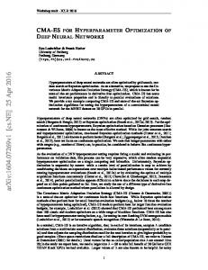
Figure 1 illustrates the optimization process. The PSO algorithm is run with the 21 training datasets. The evaluation of the hyper-parameters uses 10-fold crossvalidation (CV). Whenever a pair of SVM hyper-parameter values is generated by the tuning technique, one model is induced for each dataset using 8 partitions (training folds). One of the remaining partitions is used to validate the induced models, and will guide the search for the best hyper-parameter values (validation fold). The final one is used to asses the predictive performance of the induced models (test fold) only, not for hyper-parameter selection. This way, each dataset has validation and testing accuracies averaged over the 10-fold CV. The fitness criteria was defined as the median validation accuracy. The PSO algorithm was implemented in R using the ”pso” package, available on CRAN6 . Since PSO is a stochastic method, the technique was run 30 times 4 5

6

attrs: the number of attributes in the dataset (except the target attribute) Those are the values that presented the median accuracy over 30 solutions found in the optimization process. See Section3.2 http://cran.r-project.org/

Meta-learning for Default Recommendation

5

Fig. 1. SVM hyper-parameter tuning process with multiple datasets.

for each training dataset, so we obtain 30 solutions. The hyper-parameters values that resulted in the best median testing accuracy, considering the training datasets and executions, are defined as the ”Optimized Default” values found by the optimization technique. Those values will be compared to the default ones provided by ML tools in Section 4. 3.3

Meta-learning system

The problem of choosing one of the default values shown in Table 2 can be viewed as a classification task, and solved using a meta-learning approach. A meta-dataset is created by extracting characteristics from the datasets and used to induce a meta-model that predicts the best set of hyper-parameters based on these data characteristics. Then, this meta-model can be applied to predict which default values are more likely to lead to good predictive SVM models for a new dataset. 3.4

Meta-data set

Each meta-example of the meta-data set is composed of meta-features and a target feature. The meta-features are extracted from the 124 datasets from the total amount of 145 (Sec. 3.1). The other 21 datasets were used to find the DF-Optimized parameter settings, and are therefore excluded in the metalearning system. Since each dataset results in one meta-example, the meta-data set contains 124 meta-examples, each one composed of 81 meta-features. Table 3 shows an overview of the meta-features obtained from these datasets, subdivided into 7 subsets. These meta-features were used before in many similar studies [14, 15, 25, 27]. For each subset of these meta-features, a different meta-data set was created to explore their utility for this task. Furthermore, we built a meta-data set merging all meta-features, referred to as ALL, and another one, referred as FEAT.SELEC., obtained using a meta-feature selection method on the subset

6

Mantovani, R.G. et al. Table 3. Classes and number of meta-features used in experiments.

Meta-features Statlog Statistical Information Landmarking Model Time Complexity Total

Num. 17 7 7 10 18 9 13 81

Description Simple measures, such as number of attributes classes and attributes. Statistics measures, such as the skewness and kurtosis. Information theory measures, such as the attributes’ entropy, and so on. The performance of some ML algorithms on the datasets Features extracted from DTs models, such as the number of leaves, nodes, rules. The execution time of some ML algorithms on these dataset. measures that analyze the complexity of a classification problem. All meta-features

ALL. Specifically, we employed the correlation rank method from R package ’FSelector’, selecting the 25% most correlated meta-features. Besides the meta-features, each meta-example has a target, whose label indicates which default hyper-parameter values should be used on the corresponding dataset. In order to define the label of the meta-examples, we run the three sets of default values (DF-LibSVM, DF-Weka, and DF-Optimized) on the 124 test datasets. The hyper-parameters values that yielded the median accuracy value over 30 executions are selected. All of the default approaches were evaluated performing 10-CV strategy on testing datasets. This procedure was repeated 30 times and the predictive performance of models assessed by the mean balanced accuracy. The Wilcoxon sign-test was applied for each pair of alternatives for the default values to assess the significance of the differences of accuracy measures per dataset. Table 4 shows the win-tie-loss results based on this significance test with a confidence level of 95%. Table 4. Win-tie-loss of the approaches for 124 datasets. Technique Win Tie Loss DF-Weka 13 21 90 DF-LibSVM 6 20 98 DF-Optimized 84 6 34

In these initial experiments, we considered the problem as binary, specially due to a small number of DF-Weka and DF-LibSVM wins and eventual ties. Thus, if the best mean accuracy for the dataset was obtained by the DFOptimized with statistical significance (Wilcoxon test) compared to the other both approaches, a meta-example receives the label ”OPTM”. Otherwise, it is labeled as ”DF”. According to this criteria, 84 of the 124 datasets were labeled with the OPTM class: the induced models presented the best predictive performance when it used the parameter values obtained by the optimization process. The other 40 meta-examples were labeled with DF class: default values provided by tools were enough. Due to the small number of meta-examples, the Leave-One-Out

Meta-learning for Default Recommendation

7

Cross-Validation (LOO-CV) methodology was adopted to evaluate the predictive performance of the meta-learners. 3.5

Meta-learner

Six ML classification algorithms were used as meta-learners: J48 Decision Tree (J48), Na¨ıve Bayes (NB), k-Nearest Neighbors (k-NN) with k = 3, Multilayer Perceptron (MLP), Random Forest (RF) and Support Vector Machines (SVM). These algorithms follow different learning paradigms, each one with a distinct bias, and may result in different predictions. An ensemble (ENS) of these classifiers was also used, with prediction defined by majority voting. The predictive performance of each meta-learner, including the ensemble, was averaged over all LOO-CV iterations/executions for four performance measures. Each meta-learner was evaluated with meta-data sets composed by meta-features extracted by different approaches, described in Table 3, and the meta-feature sets ALL, which combines all meta-features, and FEAT.SELEC., which applies feature selection to ALL.

4

Experimental results

The predictive performance of models induced using the optimized default values for SVMs were compared with hyper-parameter values provided by SVMs tools. This comparison was performed by applying the Friedman statistical test and the Nemenyi post-hoc test with a confidence level of 95%. According to the test, the hyper-parameter values optimized by the PSO technique for several datasets (DF-Optimized) led to SVMs models with significantly better predictive performance than the default values provided by both SVMs tools (DF-Weka and DF-LibSVM) (see Table 4). Moreover, the test showed that there is no significance difference between the performance of DF-Weka and DF-LibSVM values. 4.1

MTL predictive performance

Table 5 summarizes the predictive performance of the meta-learners for different sets of meta-features. The first column identifies the meta-learning algorithm. The second column shows the meta-feature set used. The other columns present the predictive performance of the meta-learner according to different predictive performance measures: balanced accuracy, precision, recall, and F-Score. A trivial classifier would have a mean balanced accuracy equal to 0.500. The performance measures of this baseline method (MAJ.CLASS ) and of a RANDOM method are included at the bottom of the Table 5. The random method selects labels randomly. The best results for each meta-feature set according to the F-score measure are highlighted. A general picture of the predictive performance of the meta-learners is provided by the F-Score measure, which is a balance between precision and recall

8

Mantovani, R.G. et al.

measures, and mean balanced classification accuracy. According to these values, the J48 algorithm using all the meta-features was the best meta-learner overall, with an F-Score of 0.821 and balanced accuracy of 0.847. The same combination of meta-learner and meta-features also achieved the best results according to the precision measure. For the recall measure, the best result was also obtained by J48 algorithm, but using the Statlog meta-features subset. 4.2

Hits and Misses

Figure 2 depicts the hits and misses of the top-10 meta-models analyzing the F-score measure. The y-axis represents the meta-models: the algorithm and the set of meta-features used in the experiments. The x-axis represents all the 124 meta-examples of the meta-data set. In the figure, a hit is represented by a light gray square, and a miss by a black one.

J48.ALL J48.FSELEC

Algorithm

J48.STLG RF.STLG RF.FSELEC ENS.COMP RF.COMP ENS.LANDM J48.COMP 0

40

80

120

Dataset

Fig. 2. Hits and misses of the top 10 meta-models regarding the F-score.

The J48 algorithm appears four times in the list, while RF and ENS appear three times each one. These results indicate the superiority of J48 for this task, differently from other similar meta-learning studies, such as [22]. The intrinsic feature selection mechanism of J48 performed slightly better than the rank correlation based method (FEAT.SELEC.), since the meta-model J48-ALL is the first in the ranking followed by ”J48.FSELEC”. Another feature selection method may further improve the meta-learners predictive performance. Figure 2 illustrates that few meta-examples were misclassified by all meta-models. In these cases, all meta-examples are labeled as DF. 4.3

Tree Analysis

The decision tree in Figure 3 was the most frequently induced model during the meta-level learning using the J48 algorithm with all meta-features and performing LOO-CV. This pruned tree was obtained in most of the experiments and kept basically the same structure with 19 nodes, of which 10 are leaf nodes, and 10 rules. The meta-features selected by J48 as the most relevant ones were:

Meta-learning for Default Recommendation

1. 2. 3. 4. 5. 6. 7. 8. 9.

9

dim: the problem dimensionality (Statlog); ktsP : kurtosis pre-processed (Statistical); f3 : maximum individual feature efficiency (Complexity); stSd : standard deviation of stump time (Landmarking); bMin: minimum level of branches (tree) (Model-based); lSd : standard deviation of leaves (Model-based); eAttr : attribute entropy (Information); staTime: the execution time of a statistical model (Time); attr : number of attributes (Statlog).

Fig. 3. Most common J48 DT with all meta-features.

It is interesting to observe that about one meta-feature from each subset was used to generate the tree. The predictive meta-feature most frequently selected as the root node was dim: the problem dimensionality, i.e., dim = attributes samples . The LibSVM library considers the dimensionality of the dataset (Table 2) to assign the γ hyper-parameter value. However, the meta-feature dim is a ratio between the number of attributes and examples. According to the tree, this ratio is close to zero, DF hyper-parameter values are already good solutions, and the pre-optimized values do not improve the model’s accuracy. However, if the execution time of a statistical model (staT ime) is superior to 68.25, it indicates that the optimized hyper-parameter values should be used. The pre-optimized values are also recommended if a standard deviation of the number of leaves generated by model-based DTs is higher than 1.

5

Conclusion

Many experiments with SVMs use default values for the hyper-parameters.Thus, a good set default values allow non-expert users to have good models with

10

Mantovani, R.G. et al.

low computational costs. This study investigated the development of a metalearning system to recommend hyper-parameter values for Support Vector Machines (SVMs) from a set of predefined default values. The meta-learning system was experimentally evaluated using 124 datasets from UCI and OpenML. Besides the default values proposed by ML tools, we used an optimization technique to define new default hyper-parameter values based on a group of datasets. The use of this new set of hyper-parameter values, referred to as optimized default values, produced significantly better models than the default values suggested by ML tools. According to the experiments to assess the performance of the meta-learning system, it is possible to create a recommendation system able to select which default values must be used for SVM hyper-parameters for classification tasks. Observing the most frequent decision tree, a small number of simple meta-features was sufficient to characterize the datasets. According to this decision tree, default values proposed by ML tools are suitable for problems with a dimensionality ratio close to zero. As future work, we intend to expand the experiments by increasing the number of datasets and meta-features and exploring other ML algorithms. We also plan to cluster datasets according to their similarities to generate better optimized hyper-parameter values. The fitness value used in experiments is an aggregate measure of performance across different datasets. It would be interesting to explore other measures such as average ranks. We pretend to build on, and make all our experiments available in OpenML [29]. Acknowledgments. The authors would like to thank CAPES, CNPq (Brazilian Agencies) for the financial support. This project is supported by S˜ao Paulo Research Foundation (FAPESP) under the grant#2012/23114-9.

References 1. Andradottir, S.: A review of random search methods. In: Fu, M.C. (ed.) Handbook of Simulation Optimization, International Series in Operations Research & Management Science, vol. 216, pp. 277 – 292. Springer New York (2015) 2. Bache, K., Lichman, M.: UCI machine learning repository (2013), http:// archive.ics.uci.edu/ml 3. Bardenet, R., Brendel, M., K´egl, B., Sebag, M.: Collaborative hyperparameter tuning. In: Dasgupta, S., Mcallester, D. (eds.) Proceedings of the 30th International Conference on Machine Learning (ICML-13). vol. 28, pp. 199–207. JMLR Workshop and Conference Proceedings (2013) 4. Bergstra, J., Yamins, D., Cox, D.D.: Making a science of model search: Hyperparameter optimization in hundreds of dimensions for vision architectures. In: Proc. 30th Intern. Conf. on Machine Learning. pp. 1–9 (2013) 5. Bergstra, J., Bengio, Y.: Random search for hyper-parameter optimization. J. Mach. Learn. Res. 13, 281–305 (Mar 2012) 6. Braga, I., do Carmo, L.P., Benatti, C.C., Monard, M.C.: A note on parameter selection for support vector machines. In: Castro, F., Gelbukh, A., Gonz´ alez, M.

Meta-learning for Default Recommendation

7. 8. 9.

10. 11.

12.

13. 14.

15.

16.

17.

18.

19.

20.

21.

22.

23.

11

(eds.) Advances in Soft Computing and Its Applications, LNCC, vol. 8266, pp. 233–244. Springer Berlin Heidelberg (2013) Brazdil, P., Giraud-Carrier, C., Soares, C., Vilalta, R.: Metalearning: Applications to Data Mining. Springer Verlag, 2 edn. (2009) Chang, C.C., Lin, C.J.: LIBSVM: a Library for Support Vector Machines (2001), software available at http://www.csie.ntu.edu.tw/~cjlin/libsvm Chang, C.C., Lin, C.J.: LIBSVM: A library for support vector machines. ACM Transactions on Intelligent Systems and Technology 2, 27:1–27:27 (2011), software available at http://www.csie.ntu.edu.tw/~cjlin/libsvm Chapelle, O., Vapnik, V., Bousquet, O., Mukherjee, S.: Choosing multiple parameters for support vector machines. Machine Learning 46(1-3), 131–159 (Mar 2002) Eitrich, T., Lang, B.: Efficient optimization of support vector machine learning parameters for unbalanced datasets. Journal of Comp. and Applied Mathematics 196(2), 425–436 (2006) Feurer, M., Springenberg, T., Hutter, F.: Initializing bayesian hyperparameter optimization via meta-learning. In: Proceedings of the Twenty-Ninth AAAI Conference on Artificial Intelligence (Jan 2015) Friedrichs, F., Igel, C.: Evolutionary tuning of multiple svm parameters. Neurocomput. 64, 107–117 (2005) Garcia, L.P.F., de Carvalho, A.C., Lorena, A.C.: Noisy data set identification. In: Pan, J.S., Polycarpou, M.M., Wo?niak, M., de Carvalho, A.C., Quintin, H., Corchado, E. (eds.) Hybrid Artificial Intelligent Systems, Lecture Notes in Computer Science, vol. 8073, pp. 629–638. Springer Berlin Heidelberg (2013) Gomes, T.A.F., Prudˆencio, R.B.C., Soares, C., Rossi, A.L.D., nd Andr´e C. P. L. F. De Carvalho: Combining meta-learning and search techniques to select parameters for support vector machines. Neurocomput. 75(1), 3–13 (Jan 2012) Hall, M., Frank, E., Holmes, G., Pfahringer, B., Reutemann, P., Witten, I.H.: The weka data mining software: An update. SIGKDD Explor. Newsl. 11(1), 10–18 (Nov 2009) Hsu, C.W., Chang, C.C., Lin, C.J.: A Practical Guide to Support Vector Classification. Department of Computer Science - National Taiwan University, Taipei, Taiwan (2007) Hutter, F., Hoos, H., Leyton-Brown, K., St¨ utzle, T.: Paramils: an automatic algorithm con- figuration framewor. Journal of Artificial Intelligence Research (36), 267–306 (2009) Hutter, F., Hoos, H.H., St¨ utzle, T.: Automatic algorithm configuration based on local search. In: Proceedings of the 22nd national conference on Artificial intelligence - Volume 2. pp. 1152–1157. AAAI’07, AAAI Press (2007) Kennedy, J.: Particle swarms: optimization based on sociocognition. In: Castro, L., Zuben, F.V. (eds.) Recent Development in Biologically Inspired Computing, pp. 235–269. Idea Group (2005) Koch, P., Bischl, B., Flasch, O., Bartz-Beielstein, T., Weihs, C., Konen, W.: Tuning and evolution of support vector kernels. Evolutionary Intelligence 5(3), 153–170 (2012) Mantovani, R.G., Rossi, A.L.D., Bischl, B., Vanschoren, J., Carvalho, A.C.P.L.F.: To tune or not to tune: recommending when to adjust svm hyper-parameters via meta-learning. In: Proceedings of 2015 International Joint Conference on Neural Network (Jul 2015) Nannen, V., Eiben, A.E.: Relevance estimation and value calibration of evolutionary algorithm parameters. In: Proc. of the 20th Intern. Joint Conf. on Art. Intelligence. pp. 975–980. IJCAI’07 (2007)

12

Mantovani, R.G. et al.

24. Reif, M., Shafait, F., Dengel, A.: Meta-learning for evolutionary parameter optimization of classifiers. Machine Learning 87, 357–380 (2012) 25. Reif, M., Shafait, F., Goldstein, M., Breuel, T., Dengel, A.: Automatic classifier selection for non-experts. Pattern Analysis and Applications 17(1), 83–96 (2014) 26. Rossi, A.L.D., Carvalho, A.C.P.L.F.: Bio-inspired optimization techniques for svm parameter tuning. In: Proceed. of 10th Brazilian Symp. on Neural Net. pp. 435– 440. IEEE Computer Society (2008) 27. Soares, C., Brazdil, P.B., Kuba, P.: A meta-learning method to select the kernel width in support vector regression. Machine Learning 54(3), 195–209 (2004) 28. Thornton, C., Hutter, F., Hoos, H.H., Leyton-Brown, K.: Auto-WEKA: Combined selection and hyperparameter optimization of classification algorithms. In: Proc. of KDD-2013. pp. 847–855 (2013) 29. Vanschoren, J., van Rijn, J.N., Bischl, B., Torgo, L.: OpenML: Networked science in machine learning. SIGKDD Explorations 15(2), 49–60 (2013)

Meta-learning for Default Recommendation Table 5. Meta-learning results using LOO-CV. Classifier J48 MLP NB 3-NN RF SVM ENS J48 MLP NB 3-NN RF SVM ENS J48 MLP NB 3-NN RF SVM ENS J48 MLP NB 3-NN RF SVM ENS J48 MLP NB 3-NN RF SVM ENS J48 MLP NB 3-NN RF SVM ENS J48 MLP NB 3-NN RF SVM ENS J48 MLP NB 3-NN RF SVM ENS J48 MLP NB 3-NN RF SVM ENS BASELINE BASELINE

Meta-features Bal. Acc. STATLOG 0.839 STATLOG 0.766 STATLOG 0.427 STATLOG 0.734 STATLOG 0.823 STATLOG 0.758 STATLOG 0.798 STATISTICAL 0.734 STATISTICAL 0.677 STATISTICAL 0.492 STATISTICAL 0.750 STATISTICAL 0.742 STATISTICAL 0.702 STATISTICAL 0.718 INFORMATION 0.806 INFORMATION 0.782 INFORMATION 0.637 INFORMATION 0.677 INFORMATION 0.782 INFORMATION 0.758 INFORMATION 0.774 LANDMARKING 0.766 LANDMARKING 0.758 LANDMARKING 0.702 LANDMARKING 0.750 LANDMARKING 0.782 LANDMARKING 0.774 LANDMARKING 0.798 MODEL 0.734 MODEL 0.734 MODEL 0.677 MODEL 0.677 MODEL 0.782 MODEL 0.734 MODEL 0.774 TIME 0.718 TIME 0.790 TIME 0.403 TIME 0.766 TIME 0.774 TIME 0.766 TIME 0.774 COMPLEXITY 0.806 COMPLEXITY 0.774 COMPLEXITY 0.750 COMPLEXITY 0.710 COMPLEXITY 0.806 COMPLEXITY 0.806 COMPLEXITY 0.815 ALL 0.847 ALL 0.718 ALL 0.573 ALL 0.766 ALL 0.806 ALL 0.782 ALL 0.782 FEAT.SELEC. 0.839 FEAT.SELEC. 0.710 FEAT.SELEC. 0.581 FEAT.SELEC. 0.774 FEAT.SELEC. 0.823 FEAT.SELEC. 0.774 FEAT.SELEC. 0.782 MAJ. CLASS 0.500 RANDOM 0.501

Precision 0.757 0.703 0.518 0.679 0.764 0.645 0.733 0.660 0.572 0.592 0.717 0.672 0.616 0.667 0.726 0.708 0.601 0.638 0.695 0.645 0.689 0.710 0.717 0.649 0.724 0.721 0.715 0.753 0.673 0.686 0.579 0.651 0.735 0.627 0.722 0.635 0.701 0.546 0.729 0.715 0.638 0.722 0.739 0.715 0.730 0.648 0.746 0.713 0.758 0.815 0.674 0.619 0.716 0.746 0.669 0.735 0.802 0.661 0.632 0.722 0.758 0.657 0.735 0.500 0.505

Recall 0.884 0.737 0.522 0.693 0.815 0.781 0.785 0.695 0.608 0.608 0.715 0.705 0.649 0.675 0.817 0.767 0.596 0.634 0.782 0.781 0.765 0.734 0.723 0.655 0.716 0.758 0.746 0.773 0.693 0.694 0.610 0.641 0.753 0.714 0.744 0.673 0.801 0.601 0.732 0.746 0.872 0.744 0.799 0.746 0.718 0.663 0.793 0.844 0.801 0.829 0.676 0.607 0.733 0.793 0.847 0.753 0.821 0.666 0.619 0.744 0.822 0.842 0.753 0.339 0.505

F-Score 0.785 0.714 0.424 0.685 0.781 0.654 0.749 0.669 0.570 0.489 0.716 0.682 0.622 0.670 0.747 0.724 0.597 0.636 0.713 0.654 0.705 0.719 0.719 0.652 0.719 0.734 0.726 0.761 0.680 0.689 0.579 0.644 0.742 0.633 0.730 0.642 0.720 0.376 0.731 0.726 0.642 0.730 0.757 0.726 0.723 0.653 0.761 0.736 0.773 0.821 0.675 0.569 0.723 0.761 0.685 0.742 0.810 0.663 0.578 0.730 0.777 0.669 0.742 0.404 0.486

13