Metabolic Algorithm with Time-varying Reaction Maps Luca Bianco, Federico Fontana, Vincenzo Manca University of Verona Department of Computer Science strada Le Grazie, 15 37134 Verona, Italy E-mail: {bianco,fontana}@sci.univr.it,
[email protected] Summary. A symbolic-based approach to modelling biochemical processes and cellular dynamics is likely to turn useful in computational biology, where attempts to represent the cell as a huge, complex dynamic system must trade with the linguistic nature of the DNA and the individual behavior of the organelles living within. The early version of the metabolic algorithm gave a first answer to the problem of representing oscillatory biological phenomena, so far being treated with traditional (differential) mathematical tools, in terms of rewriting systems. We are now working on a further version of this algorithm, in which the rule application is tuned by reaction maps depending on the specific phenomenon under consideration. Successful simulations of the Brusselator, the Lotka-Volterra population dynamics and the PKC activation foster potential applications of the algorithm in systems biology.
1 Introduction Symbolic rewriting has traditionally been used to study and classify formal languages [18]. It was some years after Chomsky’s fundamental discoveries that rewriting systems began to be applied to the study of the growth of some simple organisms and to the analysis of biological structures [9, 15]. These early applications of rewriting to practical case studies taken from the real world demonstrated the potential ability of a properly defined formal construct to represent, in principle, the development of at least some biological species. Such constructs, in fact, move step by step toward the definition of a language/structure until their computation terminates, hence their application to species in development emphasized the possibility for formal systems to figure out not only classes of languages, but also the paths along which their final structure takes form during the system evolution. Recently, a research line has started which focuses on the rewriting system dynamic activity instead of its expressive power evaluated in terms of language
44
L. Bianco, F. Fontana, V. Manca
types [20, 3, 11]. This line has been stimulated in an attempt to capture, by means of rewriting systems, the dynamics of a biochemical process. In this attempt a novel construct known as P system has come useful, provided its capability to represent several structural aspects of the cell along with many intra- and extra-cellular communication mechanisms [16, 4]. Such a dynamic perspective on rewriting employing P systems has already led to alternative representations of different biological dynamics [1, 19] and to new models of important pathological processes [3, 14]. In [3, 11] we have started to develop a metabolic algorithm that introduced a new perspective in the rewriting mechanism of P systems: 1. rules are not applied to objects. Rather, they are applied to populations of objects; 2. rules are specified along with reactivities. Every reactivity denotes the ability of the corresponding rule to compete against other rules in capturing part of a population, on which the reaction is performed. We have gone further in this perspective, by associating every reactivity to a map that depends on the state of the system. Moreover we have added a strategy for partitioning the objects in the system at every transition, depending on the relative magnitude of every reactivity. The performance shown by the metabolic algorithm in the simulation of wellknown biochemical models, such as the Lotka-Volterra population dynamics [10, 21], the BZ chemical reaction [5], and the PKC activation process [2], fosters potential applications in critical open problems dealt with by systems biology [7]. Simulation in progress are confirming the effectiveness of the algorithm in modelling even more complex biochemical processes, such as those that evoke circadian rhythms in living bodies [8].
2 Metabolic Algorithm As we have told in the introduction, the metabolic algorithm is built on P systems. For the sake of simplicity here, and in the following, we hypothesize that this system is made of just one membrane. In Section 5 we will briefly discuss the formal extensions needed to cope with more membranes. To provide our algorithm with flexibility we will guarantee the fulfillment of the two following principles at any transition of a P system Π, working on the alphabet A = {X, Y, . . . , Z} and provided with rules r, s, . . . , w ∈ R: •
•
increasing the activity of a rule implies a proportional decrease of the rewriting activity of other rules sharing the same symbols. This condition reflects the concurrency among rules over a finite set of objects in the system; the applicability of rules is limited by those objects, whose availability in the system is low. This condition reflects a constraint on resources.
Metabolic Algorithm with Time-varying Reaction Maps
45
In the following we will reformulate these two points in quantitative terms. In the early version of the metabolic algorithm we had postulated that proper reactivity constants affected the rewriting activity of every rule, respectively, in a way that a larger reactivity constant defined a higher rewriting activity of the corresponding rule. Then, this activity was properly limited by defining a population on which a rule r : αr → βr , transforming the string αr ∈ A∗ into a new string βr ∈ A∗ , could be applied during a transition depending on the number of objects available in the system immediately before that transition. The new version of the metabolic algorithm requires, firstly, to recognize the state of the system. This state is used inside so-called reaction maps which generalize the former reactivity constants into time-varying functions. Once we have such maps at hand we will let the rules work according to the relative reactivity expressed by every map, meanwhile limiting this power to avoid over-consumption of the objects in the system. Finally, a simple stochastic method will be adopted to decide how to treat individual objects in the system, for which the procedure described so far does not take a definite decision. More in general, introducing stochastic properties in an algorithm can turn out to be particularly desirable when the dynamics is highly influenced by few molecules [6]. 2.1 State of the System In classical dynamic systems the values assumed along time by every variable usually form the state of the system. In a similar way, here we postulate that at every discrete time t the number of objects of each type is well defined for every membrane. Formally, the state of the system at time t is identified by a function qt :
A −→ N,
(1)
where A is the alphabet of the P system. For instance, qt (X) gives the amount of objects X available in the system at time t. Note that we will usually omit to denote t, except for those cases in which specifying the time turns out to be convenient. The state, hence, can be read by applying qt to every symbol of the alphabet. The set of all states assumed along time by the system is expressed by: Q = {qt | t ∈ N}.
(2)
This set, then, contains the complete information on the evolution of the system. Further insight on the state is not possible since qt is the only probe we can use to observe it. 2.2 Reaction Maps As opposite to the early metabolic algorithm [3] in which the reactivity constants had a direct (and time invariant) role on rewriting, here we generalize such constants into reaction maps, one for each rule, in a way that every reaction map gives
46
L. Bianco, F. Fontana, V. Manca
the reactivity that the corresponding rule has when the system is in a given state. It follows that such maps are time varying, i.e., they in general specify different reactivities in correspondence of different temporal steps. Formally speaking, for each rule r we define a reaction map Fr that maps states into real numbers: Fr : Q −→ R. (3) Since q is defined at any temporal step, the application of a reaction map Fr ultimately results in a positive real number that we will take as the reactivity of r in q. Such maps allow for a wide choice of possible definitions depending on the biological phenomenon under analysis: according to the traditional formulation of dynamic system it is not restrictive to consider real functions that in their structure include the state of the system plus factors such as the reactivity constants mentioned at the beginning of this section. As an example, consider a rewriting system having an alphabet made of five symbols, A = {A, B, C, D, E}, and two rules, r and s: k
r:
ABB →r AC
s:
AE →s BD
k
(4)
in which, consistently with notations traditionally adopted in biochemistry, we have specified constant reactivities (kr and ks ) that are peculiar to each rule— they could be, for example, kinetic parameters related to the chemical reactions respectively associated to these rules. Possible structures of the reaction maps might be the following ones: • simple reactivity constants Fr = kr Fs = ks •
reactivities driven by the law of mass action Fr = kr q(A)q(B) Fs = ks q(A)q(E)
•
reactivities depending on only the largest number of objects in the system that are visible to the rule Fr = max{q(A), q(B)} Fs = max{q(A), q(E)}
• reactivities depending on an external promoter, like an enzyme capable of activating the reaction Fr = q(D) Fs = {q(D)}2
Metabolic Algorithm with Time-varying Reaction Maps
47
In the following we will pick up this example as long as we need to illustrate the principles of the algorithm. 2.3 Reaction Weights Reaction maps are not used directly, as reactivities. Rather, their activity is proportionally distributed among the rules by means of so-called reaction weights. Every reaction weight then gives, for each symbol, a population amount a rule applies to in order to proportionally consume the corresponding object. By denoting with α(i) the ith symbol in a string α, with |α| the length of the same string, and with ¡ |α|X¢the number of occurrences of X in α, then we define the reaction weight Wr αr (i) for r : αr → βr with respect to the symbol αr (i). Normalization can be straightforwardly expressed in quantitative terms if we think that all rules co-operate, each one with its own reactivity, to consume all available objects. Thus, it must be: X ¡ ¢ Wρ X = 1 ∀ X ∈ A (5) ρ∈R | X∈αρ
that is, for each symbol the sum of the reaction weights made over the rules containing that symbol in their left part equals unity. Holding this constraint, we can define the reaction weights for each r ∈ R as ¡ ¢ Wr αr (i) =
Fr X
Fρ
,
i = 1, . . . , |αr |
(6)
ρ∈R | αr (i)∈αρ
Note that, similarly to what happens in (5), we sum at the denominator over the rules containing the symbol αr (i) in their left part. Returning to our example, we have to compute Wr (A), Wr (B), Ws (A), Ws (E): Fr = 1 Wr (A) = F F+r F Wr (B) = F r s r s Ws (A) = F F+s F Ws (E) = F Fs = 1 r s
(7)
2.4 Limitation, Rounding and State Transition For what we have said in the above, the available objects are consumed proportionally to the reaction weights. Then, in our example we have to choose whether to consume Wr (A)q(A) or Wr (B)q(B) (8) objects using r, and Ws (A)q(A)
or
Ws (E)q(E)
(9)
48
L. Bianco, F. Fontana, V. Manca
using s—provided for simplicity that all values in (8) and (9) are integer. The right choice is figured out by considering that every rule cannot consume more than the amount of the (reactant) object, taken with its own multiplicity in the reaction, whose availability in the system is lowest. Limitation, then, comes out for every rule by minimizing among all reactants participating to it: ¡ ¢ n ¡ ¢ q αr (i) o Λr = min Wr αr (i) ¯¯ ¯¯ (10) i=1,...,|αr | αr αr (i) Still, Λr is a real number. As opposite to this, a genuine object-based rewriting system must restrict the rule application domain to integer values. Instead of, for instance, rounding the minima obtained by (10), we prefer the following policy (later we will understand why): for every rule, compare the fractional part frac(Λr ) of Λr to a random variable vr defined between 0 and 1, and choose the floor of Λr if this fraction is smaller, the ceiling otherwise. In this way, new rounded minima result to be equal to: ½ floor(Λr ) , frac(Λr ) ≤ vr Λr = . (11) ceil(Λr ) , frac(Λr ) > vr As a result of this step we obtain the set {Λr , r ∈ R}, containing the number of objects each rule will be applied to. In conclusion, for every symbol X ∈ A the change in the number of objects due to r is equal to the stoichiometric factor of r, equal to |βr |X − |αr |X , times the value Λr : ∆r (X) = Λr (|βr |X − |αr |X ) (12) It descends that for every symbol X ∈ A the state evolves according to the following formula: X qt+1 (X) = qt (X) + ∆r (X) (13) r∈R
Again in our example, let us suppose that at time t it is q(A) = q(B) = q(C) = q(D) = q(E) = q˜, furthermore Fr = 3/4 Fs . Then, n
3/4Fs 1 o 3 q˜, q˜ = q˜ 3/4Fs + Fs 2 7 o 4 n Fs Λs = min q˜, q˜ = q˜ 3/4Fs + Fs 7
Λr = min
After rounding Λr and Λs (here, for simplicity, we suppose to have found integers already at the limitation step) we have 3 q˜ (1 − 1) = 0 7 6 3 ∆r (B) = q˜ (0 − 2) = − q˜ 7 7 ∆r (A) =
Metabolic Algorithm with Time-varying Reaction Maps
∆r (C) = ∆s (A) = ∆s (B) = ∆s (D) = ∆s (E) =
49
3 3 q˜ (1 − 0) = q˜ 7 7 4 4 q˜ (0 − 1) = − q˜ 7 7 4 4 q˜ (1 − 0) = q˜ 7 7 4 4 q˜ (1 − 0) = q˜ 7 7 4 4 q˜ (0 − 1) = − q˜ 7 7
in a way that 3 4 q˜ = q˜ 7 7 ³ 6 4´ 5 q˜ + − + q˜ = q˜ 7 7 7 3 10 q˜ + q˜ = q˜ 7 7 11 4 q˜ + q˜ = q˜ 7 7 4 3 q˜ − q˜ = q˜ 7 7
qt+1 (A) = q˜ − qt+1 (B) = qt+1 (C) = qt+1 (D) = qt+1 (E) =
From the last equations it follows that X X qt+1 (X) = 32/7 q˜ < qt (X) = 5˜ q X∈A
X∈A
Interesting to see, in this system the total number of objects cannot increase along time. In other words in our example the following relation holds: X X qt+1 (X) ≤ qt (X) X∈A
X∈A
3 Flexibility of the Algorithm The proposed algorithm has two basic access points where parameters can be put into: the reaction maps, and the stochastic properties of vr . •
Reaction maps can be defined with relative freedom, and even changed during the process according to the specific phenomenon under study. Their activity, in fact, is in any case normalized by the reaction weights. Occasionally some maps may result in null values: in this case reaction weights might arise in the form 0/0, and proper strategies must be put into action to handle them properly. Reaction maps, in conclusion, enable the fine control of the macroscopic, i.e., deterministic part of the process.
50
•
L. Bianco, F. Fontana, V. Manca
Conversely, the statistics of vr has consequences on the system behavior that become as more important, as fewer objects are present in the system. In other words it influences the stochastic part of the process, i.e., its unpredictability in front of individual drifts from the average behavior. Although further research must be carried out to shift the metabolic algorithm closer to stochastic methods used in biochemistry [17], nevertheless the control of vr already allows to handle, at least to some extent, an interesting property of most discrete population dynamics, according to which the decision taken by an individual becomes as more crucial, as less populated the system is [6]. This feature is evident in the simulation of the Lotka-Volterra dynamics proposed in the following. The rounding policy expressed by (11) does not prevent that the resulting application of rules exceeds the available resources in the system. As an example suppose that, during a transition, it happens that Λr ≥ Λr for each r ∈ R: in this case it is likely that the consequent application of the rules over-consumes at least some objects available in the system. To prevent this we must check that X Λr |αr |X ≤ q(X) ∀ X ∈ A (14) r∈R
otherwise the set of minima must be computed again. In first approximation vr can be chosen to have a uniform distribution. We will present here an example in which a different choice of the random variable leads to more accurate simulation results. 3.1 Transparent Rules The metabolic algorithm allows to tune the activity of rules. Tuning is achieved by adding in the system so-called transparent rules, i.e., rules in the form αr → αr . Proper reaction maps can be selected to put such transparent rules in concurrence with the other, effective rules sharing common reactants. In this way, during a transition of the system every rule is applied as less intensively, as larger the reactivity value expressed by a concurrent transparent rule is. k For instance, let us add a rule t : A →t A in the system expressed by (4). This leads to the following reaction weights: Fr r Wr (A) = F + F Fs + Ft Wr (B) = Fr = 1 r Fs s Ws (A) = F + F Fs + Ft Ws (E) = Fs = 1 r
(15)
Note that we can omit to compute Wt (A) due to the transparency of the corresponding rule. Clearly, Ft tunes the action of r and s over the symbol A. In the limit case Ft = ∞ the rule t inhibits the action of r and s over A, since in this case we have Wr (A) = Ws (A) = 0. Finally, a rule t : ABE → ABE would inhibit both r and s in the same limit case.
Metabolic Algorithm with Time-varying Reaction Maps
51
Transparent rules add further flexibility to the algorithm. In particular, they allow to observe the system evolution with the desired degree of resolution regardless of any consideration about the granularity of the temporal step. Changes in resolution are instead obtained by “hiding” objects to the system evolution by means of transparent rules. The way transparent rules work reflects an inherent attitude of the metabolic algorithm to scale its own resolution not along the time dimension, i.e., by means of a temporal scaling factor as it happens in most numerical methods. Rather, resolution is scaled by adapting the size of populations to the degree of precision expected for the experiment.
4 Results We show results coming from the predator-prey population dynamics, the Brusselator, and the PKC activation process. 4.1 Predator-Prey Population Dynamics The classic Lotka-Volterra population dynamics [10, 21] can be described by a simple set of rewriting rules in which X are preys and Y predators: k
r r : X −→ XX prey reproduction
k
s s : XY −→ Y Y predator reproduction
kt
t : Y −→ λ
(16)
predator death
Here, we can tune the activity of every rule by selecting proper reactivity constants kr , ks and kt proportional to the rate of reproduction and death of both predators and preys. We postulate Fs to be constantly proportional to ks times the maximum number between preys and predators, max{q(X), q(Y )}, that are present in the population at any system transition. Conversely, the remaining reaction maps are set to be constantly equal to the corresponding reactivity constants: Fr = kr Fs = ks max{q(X), q(Y )} Ft = kt
(17)
Moreover we add transparent rules accounting for preys that are not reproducing or being consumed and for predators that are not eating or dyeing: k
u u : X −→ X prey standing by
k
v v : Y −→ Y predator standing by
The set of reaction weights is then equal to
(18)
52
L. Bianco, F. Fontana, V. Manca
Fr Wr (X) = F + F r s + Fu Fs s Ws (X) = F + F Ws (Y ) = F + F Ft + Fv r s + Fu s
(19)
Ft Wt (Y ) = F + F s t + Fv Noticing that |αs |X = |αs |Y = 1, then the minimum between weighted preys and weighted predators must be calculated at each system transition as n Λs = min
ks max{q(X), q(Y )} q(X), kr + ku + ks max{q(X), q(Y )} o ks max{q(X), q(Y )} q(Y ) kt + kv + ks max{q(X), q(Y )}
(20)
If we in particular choose kr = kt and ku = kv this minimum becomes equal to Λs =
ks max{q(X), q(Y )} min{q(X), q(Y )} kr + ku + ks max{q(X), q(Y )} ks q(X)q(Y ) = kr + ku + ks max{q(X), q(Y )}
(21)
In this case we have kr q(X) kr + ku + ks max{q(X), q(Y )} ks Λs = q(X)q(Y ) kr + ku + ks max{q(X), q(Y )} kr Λt = q(Y ) kr + ku + ks max{q(X), q(Y )}
Λr =
(22)
Interesting to notice, these values resemble the terms proposed by Lotka-Volterra in its model of population dynamics. The choice made (not by chance) in (17), then, adds insight on the meaning of the population dynamics equations in the context of a rewriting system whose objects play the role of either preys or predators. Finally we check that the rounding procedure, making use of uniform random variables, does not produce over-consuming applications of the rules: Λr + Λs ≤ q(X)
(23)
Λs + Λt ≤ q(Y ) (though, the existence of u and v makes this possibility remote). A plot of the initial dynamic behavior of the predator-prey model is depicted in Figure 1 and, after 136000 observation slots, in Figure 2. These plots come out when we set kr = kt = 3 · 10−2 , ks = 4 · 10−5 , and ku = kv = 5. Using
Metabolic Algorithm with Time-varying Reaction Maps
53
1100 preys predators 1000
populations
900
800
700
600
500
400
0
1000
2000
3000
4000 step
5000
6000
7000
8000
Fig. 1. Predator-prey initial dynamics.
these parameters, along with initial conditions q(X) = q(Y ) = 900, the system exhibits an interesting oscillating behavior. The oscillation can evolve to the death of both species, as in Figure 2, or to the death of the predators solely. The longterm evolution in fact depends on single events taking place when few individuals, either preys or predators, are present in the system. Such a long-term behavior emphasizes the importance of a careful description of not only the reactivities, but also the relationships existing between individuals: the nature of these relationships can completely change the overall system evolution. 4.2 Brusselator The Belousov-Zhabotinskii (BZ) reaction has represented a milestone in the history of physical chemistry, as it disclosed the previously unrecognized existence of oscillatory chemical phenomena [5]. A simple model of the BZ reaction is realized by the Brusselator [20]:
54
L. Bianco, F. Fontana, V. Manca
8000 preys predators
7000 6000
populations
5000 4000 3000 2000 1000 0 1.36
1.37
1.38
1.39
1.4 step
1.41
1.42
1.43
1.44 5
x 10
Fig. 2. Predator-prey dynamics after 136000 observation slots.
r:
λ
k
r −→
X
reactant in
ks
s : XXY −→ XXX compound into reactant k
Y
reactant into product
k
λ
reactant dissolving
t:
X
t −→
u:
X
u −→
(24)
This set of rules accounts for the fact that the reactant X either turns into a product Y or participates in transforming the product back to the reactant itself. As opposite to the predator-prey model, the Brusselator includes a constant incoming and dissolving of reactant in the system. The literature on the Brusselator suggests that the reaction activity depends on the concentrations of chemical elements according to the law of mass action. We then define the following reaction maps: Fr = kr Fs = ks {q(X)}2 q(Y ) Ft = kt q(X) Fu = ku q(X)
(25)
Metabolic Algorithm with Time-varying Reaction Maps
55
It must be noticed that rules containing λ in their left part do not compete for a limited availability of reactant or for a bounded population, by definition. For this reason they act unconstrained, i.e., no reaction weight holds for any of them. Hence, we come up with the following reaction weights in which r is not considered: Fs Fs Ws (X) = F + F + F Ws (Y ) = F = 1 s
t
u
s
Ft Wt (X) = F + F s t + Fu
(26)
u Wu (X) = F + F Ft + Fu s
Again we have to minimize only over s at any system transition: n Λs = min
o 1 Fs (X) q(X), q(Y ) |αs |X Fs (X) + Ft (X) + Fu (X)
(27)
so that in the end we have Λr = kr
o ks {q(X)}2 , 1 2 kt + ku + ks q(X)q(Y ) kt Λt = q(X) kt + ku + ks q(X)q(Y ) ku Λu = q(X) kt + ku + ks q(X)q(Y ) Λs = q(Y ) min
n1
(28)
Finally we check out that the rounding procedure does not produce overconsuming applications of rules. By (14) it turns out that checking over X is sufficient: 2Λs + Λt + Λu ≤ q(X) (29) A plot of the dynamic behavior of our rewriting system modelling the Brusselator, in which we have set kr = 10, ks = 9, kt = 200, ku = 5, and initially q(X) = 1 and q(Y ) = 10, is depicted in Figure 3. The overall behavior is satisfactory if compared to real experiments conducted over the BZ reaction [5]. An artifact, visible in the center part of the plot, arises after around 1350 steps consisting in a constant climb of the concentration of the reactant. This fact reveals the existence of periods in which the reaction goes in a stand-by situation, and then restarts with the oscillatory dynamic behavior. Interesting to say, a major reduction of this artifact has been achieved by changing the properties of the random variables devoted to round the number of times every rule is applied: by altering their uniform probability so to privilege truncation and discourage rounding toward one, then constant rise-ups of the reactant are almost completely removed.
56
L. Bianco, F. Fontana, V. Manca
5000
reactant product
concentration
4000
3000
2000
1000
0 1320
1340
1360 step
1380
1400
1420
Fig. 3. Brusselator dynamics.
As in the predator-prey model we notice that individual differences in the rule application, occurring when there are few reactant and/or product objects, turn into differences in the system behavior. Though, the BZ reaction is more robust against perturbations and exhibits an asymptotic long-term behavior, that is, individual events affect only the short-term evolution: as opposite to a Lotka-Volterra’s population dynamics, in which the evolution of the system entirely depends on its internal state, the Brusselator is, in fact, driven by a constant incoming and dissolving of the reactant, accounted for respectively by r and u. This streaming activity adds inherent robustness to the model of a BZ reaction. 4.3 PKC activation As another case study, we consider here a simple signal transduction network describing the activation of the protein kinase C (PKC) [12, 13]. The importance of this process is due to the fact that PKC mediates many cellular responses to extracellular stimuli and is involved in several regulatory phosphorylations dealing with proliferation, apoptosis and differentiation. PKC activation is elicited by the allosteric effect of calcium ions (Ca), whose affinity is increased by other agents such as arachidonic acid (AA) and diacylglycerol (DAG).
Metabolic Algorithm with Time-varying Reaction Maps
57
We refer to the PKC activation model discussed in [2], to which we send the reader for further details. We have translated this model into the following set of rules: r1 : P KC − i → P KC − a r2 : P KC − a → P KC − i r3 : P KC − i AA → P KC − aA r4 : P KC − aA → P KC − i AA r5 : Ca.P KC → P KC − aC r6 : P KC − aC → Ca.P KC r7 : Ca.P KC AA → P KC − aCA r8 : P KC − aCA → Ca.P KC AA r9 : DAG.Ca.P KC → P KC − aD r10 : P KC − aD → DAG.Ca.P KC (30) r11 : AA.DAG.P KC → P KC − aAD r12 : P KC − aAD → AA.DAG.P KC r13 : P KC − i Ca → Ca.P KC r14 : Ca.P KC → P KC − i Ca r15 : Ca.P KC DAG → DAG.Ca.P KC r16 : DAG.Ca.P KC → Ca.P KC DAG r17 : DAG.P KC AA → AA.DAG.P KC r18 : AA.DAG.P KC → DAG.P KC AA r19 : P KC − i DAG → DAG.P KC r20 : DAG.P KC → P KC − i DAG in which AA, Ca, and DAG have the meaning introduced previously and we use the symbols P KC−i and P KC−a to denote respectively the inactivated and activated form of protein kinase C. All remaining symbols represent intermediate complexes. Moreover, for every object X of the system we have introduced a transparent rule of the form X → X (not represented in the set of equations above). Note that the rules just expressed represent biochemical reactions mediated by enzymes. For this reason each rule ri is coupled with a rate constant ki . The rate constants used in our simulations are taken directly from [2] and are summarized below: k1 = 50 k4 = 2 · 10−10 k7 = 0.1 k10 = 1 k13 = 0.5 k16 = 1.3333 · 10−8 k19 = 0.1
k2 = 1 k3 = 0.1 k5 = 3.5026 k6 = 1.2705 k8 = 2 · 10−9 k9 = 0.1 k11 = 0.2 k12 = 2 k14 = 1 · 10−6 k15 = 8.6348 k17 = 2 k18 = 3 · 10−8 −9 k20 = 1 · 10
(31)
For every rule ri we define a reactivity map to be simply the corresponding rate ki : Fri = ki , i = 1, . . . , 20 (32)
58
L. Bianco, F. Fontana, V. Manca 100
90 Ca PKC−a DAG PKC−i
80
concentration
70
60
50
40
30
20
10
0
0
5
10
15 step
20
25
30
Fig. 4. PKC activation dynamics. The order of the elements in the legend is the same as the order of their final concentrations within the plot.
meanwhile we associate a constant reactivity map to each transparent rule, in our case F = 50. These reactivity maps are quite simple but in the future we intend to investigate the effectiveness of more complex reactivity maps in the case of the PKC model. The description of the whole set of weights Wri , that can be calculated object by object in the way introduced in previous sections, is omitted. Rather, we present some simulation results obtained using our algorithm. In Figure 4 we see that, in accordance with results obtained in [2], P KC − i decreases to zero while P KC − a grows up until reaching a stationary maximum. Figure 5 represents the characteristic dynamics of the diacylglycerol-protein kinase C (DAG.PKC) complex.
5 Discussion All rules discussed so far do not present any target specification. This aspect needs further discussion due to its importance. Let’s consider the following rule r, present in a membrane wi :
Metabolic Algorithm with Time-varying Reaction Maps
59
0.08 DAGPKC 0.07
0.06
concentration
0.05
0.04
0.03
0.02
0.01
0
0
10
20
30
40
50 step
60
70
80
90
100
Fig. 5. DAG.PKC complex dynamics.
AB → BINj C
,
Fr
where Fr is the reactivity map associated to r. Its meaning is the following: whenever A joins B inside wi , they combine and produce an object C inside the same membrane, meanwhile an object B leaves wi and reaches the membrane wj . In such a way r affects objects that are present in two different membranes. In particular, from a structural viewpoint, the elements B that are present in wi have to be distinguished from the elements B that are present in wj (and, in fact, this is the effect of compartmentalization). For this reason r originates four metabolic equations describing the behavior of its four distinct elements: ∆r (Awi ) = −Λr,wi ∆r (Bwi ) = −Λr,wi ∆r (Bwj ) = +Λr,wi ∆r (Cwi ) = +Λr,wi where we have introduced the label of the membrane containing every element as subscript. In this way we can see that the variation due to r on the objects B placed inside wj , i.e., ∆r (Bwj ), depends on the concentrations of A and B located in wi
60
L. Bianco, F. Fontana, V. Manca
as stated by the subscript notation (note that this dependence is hidden behind the Λr factor). This simple evolution rule is powerful enough to show that movements of objects between membranes can be handled easily by considering, as distinct elements, two objects of the same type located in different regions. This additional information introduces a notational overhead of targeting every object with the label of the membrane containing the respective object. On the other hand it does not introduce any conceptual complication. The case in which elements appearing in the antecedent of the rule are placed inside different membranes can be handled similarly. The only difference that must be taken into account is that the set of weights has to be calculated by considering, in principle, the whole set of rules of the P system rather than the set of rules of a single membrane.
6 Conclusion and Ongoing Research Systems biology demands for novel procedures capable of representing biological processes with both accuracy and flexibility. In front of a huge and well-rooted family of numerical schemes, traditionally devoted to figure out the dynamics of systems described by differential equations, alternative algorithms based on a symbolic representation of the phenomena promise to deal more naturally with the structural characteristics of the biomolecules and with the biochemical reactions such molecules give rise to. By using the same kind of representation, our algorithm moreover seems to handle in a straightforward and efficient way those conditions in which few molecules have an important impact on the system dynamics, where most traditional numerical strategies are no longer effective and must be substituted by stochastic algorithms. Successful simulations conducted on two paradigmatic nonlinear processes in biochemistry, namely the Lotka-Volterra population dynamics and the BZ reaction, plus the experiment conducted with the PKC activation process, ask for further test the potential of the metabolic algorithm. Our present research aims to simulate some fundamental signal transduction networks, in particular the PER and TIM cycle in the circadian oscillation in Drosophila.
References 1. D. Besozzi, G. Ciobanu: A P system description of the sodium-potassium pump. In Membrane Computing, 5th International Workshop, WMC 2004 (G. Mauri, G. P˘ aun, M.J. P´erez–Jim´enez, G. Rozenberg, A. Salomaa, eds.), LNCS 3365, Springer-Verlag, Berlin, 2005, 210–223. 2. U.S. Bhalla, R. Iyengar: Emergent properties of networks of biological signaling pathways. Science, 283 (January 1999), 381–387. 3. L. Bianco, F. Fontana, G. Franco, V. Manca: P systems for biological dynamics. In [4].
Metabolic Algorithm with Time-varying Reaction Maps
61
4. G. Ciobanu, Gh. P˘ aun, M.J. P´erez–Jim´enez, eds.: Applications of Membrane Computing. Springer, Berlin, 2005. 5. I.R. Epstein, K. Showalter: Nonlinear chemical dynamics: Oscillations, patterns, and chaos. J. Phys. Chem., 100, 31 (1996), 13132–13147. 6. A. Goldbeter: Computational approaches to cellular rhythms. Nature, 420 (November 2002), 238–244. 7. H. Kitano: Computational systems biology. Nature, 420 (November 2002), 206–210. 8. J.C. Leloup, A. Goldbeter: A model for circadian rhythms in Drosophila incorporating the formation of a complex between the PER and TIM proteins. J. of Biological Rhythms, 13, 1 (1998), 70–87. 9. A. Lindenmayer: Mathematical models for cellular interaction in development. Part I and part II. J. of Theoretical Biology, 18 (1968), 280–315. 10. A.J. Lotka. Undamped oscillations derived from the law of mass action. J. Am. Chem. Soc., 42 (1920), 1595–1599. 11. V. Manca, L. Bianco, F. Fontana: Evolutions and oscillations of P systems: Theoretical considerations and applications to biochemical phenomena. In Membrane Computing, 5th International Workshop, WMC 2004 (G. Mauri, Gh. P˘ aun, M.J. P´erezJim´enez, G. Rozenberg, A. Salomaa, eds.), LNCS 3365, Springer-Verlag, Berlin, 2005, 63–84. 12. A.C. Newton: Protein Kinase C: Structure, function, and regulation. J. Biol. Chem., 270 (1995), 28495–29498. 13. K. Ohkusu: Elucidation of the protein kinase C-dependent apoptosis pathway in distinct subsets of T lymphocytes in mrl-lpr/lpr mice. Eur. J. Immunol., 25 (995), 3180. 14. M.J. Perez-Jimenez, F.J. Romero-Campero: Modelling EGFR signalling network using continuous membrane systems. Third Workshop on Computational Methods in Systems Biology, Edinburgh, 2005. 15. P. Prusinkiewicz, M. Hammel, J. Hanan, R. Mech: Visual models of plant development. In Handbook of Formal Languages (G. Rozenberg, A. Salomaa, eds.), volume III: Beyond Words, Springer-Verlag, Berlin, 1997, 535–597. 16. Gh. P˘ aun: Computing with membranes. J. Comput. System Sci., 61, 1 (2000), 108– 143. 17. C.V. Rao, D.N. Wolf, A.P. Arkin: Control, exploitation and tolerance of intracellular noise. Nature, 420 (November 2002), 231–237. 18. G. Rozenberg, A. Salomaa, eds.: Handbook of Formal Languages. Springer-Verlag, Berlin, 1997. 19. I. Stamatopoulou, M. Gheorghe, P. Kefalas: Modelling dynamic organization of biology-inspired multi-agent systems with communicating x-machines and population p systems. In Membrane Computing, 5th International Workshop, WMC 2004 (G. Mauri, Gh. P˘ aun, M.J. P´erez-Jim´enez, G. Rozenberg, A. Salomaa, eds.), LNCS 3365, Springer-Verlag, Berlin, 2005, 389–403. 20. Y. Suzuki, H. Tanaka: Chemical oscillation in symbolic chemical systems and its behavioral pattern. In Proc. International Conference on Complex Systems (Y. BarYam, ed.), Nashua, NH, September 1997. 21. V. Volterra: Fluctuations in the abundance of a species considered mathematically. Nature, 118 (1926), 558–560.