Peter S. Gural. Abstract. A meteor ..... Jenniskens, P.M., Butow, S.J., Fonda, M. (2000): The 1999 Leonid Multi-Instrument Aircraft. Campaign â An Early Review ...
Proceedings IMC Cerkno 2001
29
Meteor Observation Simulation Tool Peter S. Gural Abstract A meteor observation simulation tool MeteorSim has been developed to study the phenomenology of meteor observations. This will form the basis for a series of articles to be published in WGN looking at the various aspects of visual and video meteor observation and analysis. This paper represents the first in the series describing the basic modelling and simulation capabilities.
1
Introduction
After the Leonid Multi-instrument Aircraft Campaign in 1999 (Jenniskens et al. 2000), a detailed analysis was performed on one videotape from a low elevation intensified CCD camera that was mounted onboard a high altitude aircraft (Gural & Jenniskens 2000). In analyzing the flux data as a function of elevation angle above the horizon it was empirically verified that the meteor counts increased as one looked lower towards the horizon. This effect was determined to be due to the lack of any magnitude losses arising from atmospheric extinction at the aircraft’s height of 11 kilometers. As part of the Leonid storm flux analysis it was decided to use a prototype meteor flux simulator developed by the author, to verify that these observations could be duplicated in a software simulation. During the course of that analysis and code development, it was realized that this new software for meteor simulation could also be used to derive an independent estimate of the Leonid stream mass ratio and spatial density from the measurements as well as predict optimal (highest flux) video camera pointing angles for future missions (Gural & Jenniskens 2000). The simulation has also been used most recently to verify several new meteor formulae (Gural 1999, Gural 2001) and point out to another meteor researcher a recently published formulation error. With refined models for magnitude losses, flight trajectory, and sensor detection response, the MeteorSim software tool could also be used to examine several aspects of meteor measurements and observations. Thus at the end of this paper is a list of future topics that will be covered in upcoming issues of WGN. Hopefully this series of articles can confirm or dispel any preconceived notions of meteor phenomenology associated with the collection and processing of data since the simulator is not limited to small sample size effects as real observations often are. At this time the author is requesting any insights, constructive criticisms, or improvements that can be made to the models governing this simulation.
2
Simulation and model descriptions
The “MeteorSim” program can be described as a Monte Carlo simulation, which propagates a random distribution of dynamically associated meteoroids into the Earth’s atmosphere. This simulation technique has been used in the past by other researchers to study the observational influences on meteor magnitude distribution index and zenith hourly rate corrections (Van der Veen 1986, Arlt 1998). Each Monte Carlo trial effectively places a randomly
30
Proceedings IMC Cerkno 2001
positioned meteoroid outside the Earth’s gravitational sphere of influence and propagates the particle along a specified radiant direction. The meteoroid is acted on only by the Earth’s gravity (geocentric flight dynamics) yielding a hyperbolic orbit, thus giving rise to the wellknown phenomena of zenith attraction. There is no modelling at this time for deceleration of the meteoroid (meteor) in the atmosphere due to drag, nor any deviation from the simple hyperbolic track. The meteoroids are initially distributed in space in a three-dimensionally uniformly random pattern bounded by the cylinder shown in Figure 1. The cylinder is taken large enough to ensure all points of an observer’s atmospheric cap down to the local horizon (defined as a meniscus between a specified begin and end height) can be reached by meteoroids originating in the cylinder. All the meteoroids initially move along parallel trajectories aligned with the radiant vector and possess identical velocities. Computations proceed by solving for the meteor’s position at any point along the trajectory given the distance relative to the Earth’s center. From that position, the azimuth and elevation of the meteor from the observer or sensor can be computed.
Figure 1: The meteoroids in space in a three-dimensionally uniformly random pattern bounded by the cylinder. The meteoroids are randomly assigned a magnitude referenced to a particle ablating at an observer’s zenith 100 kilometers above the Earth’s surface. The magnitude distribution follows the classical number density formula n(magnitude) = N · r (magnitude−lm) where r is the magnitude ratio for the stream, lm the limiting magnitude, and N is the total number of meteoroids of magnitude lm. To quickly pull a random draw for the magnitude assignment to each meteor, a large table of magnitudes is created with the appropriate r-factor distribution and a uniform random number generator selects the position in the table for the draw. If k is the index for the table of length M and xm is to be the brightest magnitude, then the table of magnitudes m(k) can be generated as follows: loge [k + (M − k) · r xm−lm ] − loge M m(k) = lm + loge r
(1)
Each meteor is assumed to have a constant magnitude during its flight from the beginning height to the ending height and is invisible outside those regions. Thus there will be some
Proceedings IMC Cerkno 2001
31
meteoroids that originate in the cylinder that do not intersect the observer’s meniscus and can never possibly be seen — just as in real life. It is also possible to determine if the meteoroid is a grazer (reaches the begin height and is above the observer’s horizon, but does not penetrate to the end height). Once a magnitude has been determined and a position defined, a magnitude loss must be taken to account for: 1. the distance of the meteor from the observer, 2. the effects of atmospheric extinction, and 3. the effects of angular velocity and its impact on CCD pixel dwell time. In the formulae below, R is the Earth’s radius, ho the observer’s height above the Earth, and θe the elevation angle of the meteor from the observer. For distance fading the loss is taken relative to a zenith height of 100 kilometers. For extinction losses the dependency is on the number of airmasses taken from tabulated values (Roth 1994). The airmass Z is computed via a line integral of the 1962 US Standard Atmospheric density (polynomial fit approximation) from the observer’s height along the elevation angle to the top of the atmosphere (this is normalized by the line integral from ground to zenith which equals one airmass). The angular velocity losses correspond to a CCD integrating pixel that only ”sees” a meteor for a fraction of the 1/60 second NTSC (1/50 second PAL) interleave period from its rapid motion across the face of the CCD. The angular velocity can be derived from the geocentric entry velocity, radiant angular distance, and meteor range. For a human observer it is not clear at this time what the loss should be to account for the speed of the meteor (is there an effective ωo for the human eye?).
m(observed) =m(k) + ∆m(distance) + ∆m(extinction) + ∆m(velocity) ¸ · d(km) ∆m(distance) =5 · log10 100(km) p d(km) = R2 − (R + ho )2 cos2 θe − (R + ho ) sin θe
∆m(extinction) = − 0.003 · Z 2 + 0.228 · Z − 0.225
(2) (3) (4) (5)
log10 ρ(kg/m3 ) = 0.082953 − h(0.034681 + h(0.0014865 − h(1.5604 · 10−5 + h(3.0649 · 10−7 − h · 4.7987 · 10−9 )))), height h in kilometers (6)
∆m(velocity) =
(
2.5 log10 0
for ω > ωo , otherwise
(7)
sin Dradiant d(km)
(8)
pixel size (radians) integration time (s)
(9)
ω = V∞ (km/s)
ωo =
ω ωo
32
Proceedings IMC Cerkno 2001
An example of the degree of extinction loss from the ground, mountaintop and an airborne platform are shown in Figure 2. Figure 3 is an example of the relative contributions of the three loss terms for an airborne platform looking 90 degrees in azimuth from the Leonid radiant at an altitude of 11 kilometers.
Figure 2: An example of the degree of extinction loss from the ground, mountaintop and an airborne platform.
Figure 3: The relative contributions of the three loss terms for an airborne platform looking 90 degrees in azimuth from the Leonid radiant at an altitude of 11 kilometers.
Proceedings IMC Cerkno 2001
33
Figure 4: A three-dimensional vector oriented geometry in which the simulation works.
The simulation works in a three-dimensional vector oriented geometry as seen in Figure 4. At any point in the hyperbolic trajectory, the azimuth, elevation, angular velocity, and magnitude of the meteor is known. Usually this is computed at the beginning and end points only. For simulations involving video cameras, the field of view is well defined with an assumed uniform sensitivity across the CCD. Thus all meteors above the sensor’s limiting magnitude are detected with unity probability. For human observers, the detection is a function of the radial angular distance d of the meteor relative to the observer’s look direction. A plot of meteor minimum magnitude and its elongation from the observer yields a simple test. That is the magnitude value must be less than (70◦ - δ)/10◦ for the meteor to be ¨ considered seen by the human eye (linear fit to the Opik, Backhouse, Hoffmeister plot in Roggemans 1989). A question to be settled is whether the meteor should be tested for detection at the midpoint of the track (brightest point in real meteor light curves) or at that point in the visible track closest in angular distance to the observer’s look direction (minimum elongation). Feed back from readers on this issue is desired as well as how to model the human eye response — is it in fact circularly symmetric, how to account for angular velocity losses, and should the magnitude test be more based on probability of detection versus elongation.
34
Proceedings IMC Cerkno 2001
3
Simulation processing steps
The simulation is comprised of a sequential series of steps to determine the visibility of each Monte Carlo drawn meteor track and accumulate the desired flux or other desired characteristic within the field of view. With modern PCs it is not unrealistic to run a billionparticle simulation and obtain statistics unprecedented in actual meteor observations. Loop over Monte Carlo starting positions of meteoroids (exo-atmospheric) Computation of the vector from observer to the meteoroid starting position Determine closest point of approach to Earth for straight-line propagation Determine closest point of approach (CPA) to Earth with zenith attraction Compute vectors to the meteor begin and end points (or begin and grazer CPA) Is the meteor above the observer’s horizon? No — go to next meteoroid Random draw on meteor’s magnitude Take the magnitude losses based on the azimuth and elevation at the end point Is the meteor brighter than the limiting magnitude? No — go to next meteoroid Is the meteor within the field of view or does the detector ”see” the meteor? Accumulate the desired statistics. End of Monte Carlo loop
4
Future study list
The following is a list of suggested studies that are possible with this meteor simulation and can be written up as a series of articles for WGN. It is the author’s request that any addition ideas or comments on the modelling be forwarded to him via email at the address listed in the IMO’s Who’s who database. The list is presented in no particular order except for the first item due to appear next in print. Next: • Validation plots and meteor characteristics of the baseline simulation. • Optimal look directions for video cameras and human observers. • Effect on meteor counts of r-factor and radiant elevation. • Effect on meteor counts of limiting magnitude and geocentric entry velocity. • Does the observed r-factor in all observing directions deviate from the incident distribution? • Frequency of grazer and pointer meteors. • High altitude advantages of low elevation pointing. • Verify the root-N error bar applied to low sample support meteor counts. • Optimal pointing for photographs — trade of flux for uniform angular velocity in FOV. • Trade-off of FOV and limiting magnitude for all-sky, video, and telescopic flux. • Telescopic counts versus ZHR. How often will you see a fireball — sporadic rates versus shower. • Monte Carlo studies of human perception. • Verify the ZHR correction formulae.
Proceedings IMC Cerkno 2001
35
References Arlt, R. (1998): WGN , 26, 239-248. Gural, P.S. (1999): A Rigorous Expression for the Angular Velocity of a Meteor WGN , 27-2, 111-114. Gural, P.S., Jenniskens, P.M. (2000): Leonid Storm Flux Analysis from One Leonid MAC Video AL50R Earth, Moon and Planets, 82-83, 221-247. Gural, P.S. (2001): Fully Correcting for the Spread in Meteor Radiant Positions due to Gravitational Attraction WGN , 29-4, 134-138. Jenniskens, P.M., Butow, S.J., Fonda, M. (2000): The 1999 Leonid Multi-Instrument Aircraft Campaign — An Early Review Earth, Moon and Planets, 82-83, 1-26. Roggemans, P. (1989): Handbook for Visual Meteor Observations, Sky Publishing Corp., 89. Roth, G.D. (1994): Compendium of Practical Astronomy, Appendix B, Table B.2 SpringerVerlag, 251. Van der Veen, P. (1986): Radiant, Journal of the Dutch Meteor Society, 6, 41-45.
Marc Gyssens and Axel Haas on the banks of the Pivka river which flows into the Postojna cave (photo: LOC).