MAY 1998
SOZZI ET AL.
461
Method for Estimation of Surface Roughness and Similarity Function of Wind Speed Vertical Profile ROBERTO SOZZI
AND
MAURIZIO FAVARON
Servizi Territorio scrl, Milan, Italy
TEODORO GEORGIADIS CNR–FISBAT, Physics and Chemistry of the Lower and Upper Atmosphere, Bologna, Italy (Manuscript received 16 January 1997, in final form 11 July 1997) ABSTRACT This study is aimed at identifying and refining a method suitable to estimate the surface roughness length (z 0 ) and the universal similarity function of the wind speed profile (C M ) based on ultrasonic anemometer measurements carried out at only one measurement height. This method does not require experimental knowledge of wind speed vertical profiles. It permits the use of experimental data obtained from a single sonic anemometer placed in the surface layer in any stability condition, thereby simplifying experimental campaigns and cost reduction. In a fixed station equipped with a sonic anemometer, it is also possible to obtain a periodic estimate of z 0 without additional ad hoc experimental campaigns; thus one can correlate the evolution of this parameter to changes that could be found over the area being studied. To prove its feasibility, the method was applied to data obtained in an experimental campaign carried out in Mexico near the northeast side of Mexico City. An ultrasonic anemometer operating at an altitude of 10 m above surface level was used. The method supplied positive results, thereby confirming its operative usefulness.
1. Introduction The earth’s surface interacts with the bottom of the planetary boundary layer (PBL) due to its natural and man-made geometric irregularities. Among other things, this interaction decreases wind speed in inverse relation to the closeness of the earth’s surface. From a quantity standpoint, this phenomena is evidenced by the wind speed vertical profile observations, which can be obtained by anemometers located in meteorological towers, by radiosoundings, or by sodar. By analyzing measurements obtained at a given point, it is possible to note that this ‘‘momentum sink’’ generally varies according to the wind direction, indicating that local earth surface conditions alone do not completely explain this interaction with the PBL. Air masses have a memory more or less intense of irregularities encountered along their passages. Since they are connected to the earth’s surface geometric status, these phenomena will evolve with it as seen over cultivated areas that radically change aspect with the change of seasons. Since one of the effects of the earth’s surface geometry is the alteration of the wind vertical profile and since the practical ap-
Corresponding author address: Dr. Teodoro Georgiadis, FISBAT– CNR, via Gobetti 101, I-40129 Bologna, Italy. E-mail:
[email protected]
q 1998 American Meteorological Society
plication of this profile is of importance, it is necessary to somehow quantify this interaction. Initially, a territory having an almost homogenous space devoid of scattered irregularities of a dimension causing noticeable wake effects (e.g., housing, forests, etc.) immediately around the observation point is considered. This condition should be persistent for a radius of a few kilometers. In such a situation, it has been noted that the vertical wind profile increases with height and wind speed tends to be nil very close to the earth’s surface, as surface irregularities are smallest. The height where this occurs is called the roughness length, z 0 . Standard values of this parameter run from a few millimeters for bare soil to a few decimeters over growthcovered surfaces. Even though z 0 is not exactly equal to the height of roughness found on the earth’s surface and encountered in the air masses’ flow, a bi–univocal relation does exist between the two. Once z 0 is determined for a wind direction, this parameter will not change with wind speed, atmospheric stability, or surface stress. It will change only if the nature of the obstacles encountered changes [e.g., change of z 0 over a period of time in areas of rising cultivation, Stull (1988)]. Strictly speaking, such statements are realistic only when the surface roughness is determined by ‘‘fixed obstacles.’’ A typical example of this type of surface is bare soil. When, on the contrary, the obstacles are ‘‘mobile,’’ they are no longer rigorously true, and
462
JOURNAL OF APPLIED METEOROLOGY
z 0 is found to be more or less dependent on wind speed (or, better, on friction velocity u*). A discussion on this subject is provided in Brutsaert (1982). The dependence is even clearer when considering water surfaces, which are well described by the Charnock model (Charnock 1955), where z 0 is directly proportional to u 2*. Recently, while analyzing experimental data collected in the Antarctic, it has been seen that ice surfaces present a surface roughness that is highly variable (by many orders of magnitude) due to the presence of mobile obstacles consisting of a fine layer of miniscule ice particles in a continual process of chaotic resuspension. Here too, z 0 was found to depend on u*, although in a far more complex manner than that indicated by the simple Charnock model. Further details on this phenomenon can be found in Bintanja and van den Broeke (1995). The present work does not deal with such situations but limits its scope to the consideration of surfaces mainly characterized by the presence of fixed obstacles. The adiabatic wind speed vertical profile is described in the well-known logarithmic law
12
u z u z 5 * ln , k z0
(1)
where u is the average wind speed at any height z, u* is friction velocity, and k is the von Ka´rma´n constant equal to 0.4. This equation can be derived from both the basic fluid dynamic equation (Stull 1988) and the similarity theory (Sorbjan 1989). If surface geometric characteristics are very different from this ideal situation and roughness elements are grouped close together, as, for example, in the presence of a forest or urban area, this parameter is no longer sufficient to describe PBL surface interaction. The socalled zero-plane displacement height d is then necessary, which is defined as the altitude above which the wind profile is again described by a similarity equation. In this case for every height z greater than d, the adiabatic equation (1) is modified as follows:
1
2
u (z 2 d) u z 5 * ln . k z0
(2)
Details on this parameter can be found in Wieringa (1993). In this work only geometrically homogeneous surfaces without obstacles that could cause noticeable wakes will be considered. From the similarity theory and experimentation, it has been found that in adiabatic situations and within the surface layer (SL) that the wind speed vertical profile can be quantified by Eq. (1). If various adiabatic profiles are known, it is possible to estimate simply the z 0 value for various wind directions. If an adiabatic wind speed vertical profile is known at N heights, methods proposed in the literature (Stull 1988) use Eq. (1) for reference and obtain a friction velocity and z 0 estimate minimizing the following minimum squares functional:
VOLUME 37
O [u 2 1uk* ln(z ) 2 uk* ln(z )2] . 2
N
F(u* , z 0 ) 5
i
i
0
(3)
i51
When M wind speed vertical profiles are available in adiabatic conditions for a given wind direction, M estimates of z 0 are obtained, and the median of these estimates can be considered the most probable values for the roughness parameters of the direction under consideration. Most methods proposed in the literature actually lead back to the above-described equation. In addition to methods based on the adiabatic wind vertical speed profile, there exist methods founded on the analysis of the standard deviation of the horizontal component of the wind speed in adiabatic conditions (Beljaars and Holtslag 1991). The method’s basis is the following similarity equation, true in adiabatic conditions:
su 5 2.5. u*
(4)
Upon substitution of the friction velocity with its expression from Eq. (1), the following equation is derived:
su 5 1/ln[z/z 0 ]. u
(5)
The latter expression defines an estimator of the roughness length parameter. When M couples (u, s u ) are available for a given wind direction, Eq. (5) can be used to obtain M estimates of z 0 ; here too the median of the estimates can be considered as the most probable roughness length value. Essentially, this is the method proposed by the U.S. Environmental Protection Agency (EPA 1987). However, during its application, remember that the constant in the right-hand part of Eq. (4) has a degree of uncertainty due to the scatter of the experimental data from which it is derived (Panofsky and Dutton 1983). In addition, Panofsky and Dutton explain how the interpretation of observed variances and standard deviations is made difficult by the lack of any standard procedure for measuring them; thus, at the lowfrequency end, an appropriate procedure should be used to eliminate low-frequency nonturbulent contributions to the variance, without filtering out the contributions of low-frequency turbulence. These remarks are far from irrelevant and demonstrate how crucial a correct application of the method is. Problems arising from the use of these methods are due to the fact that there are few really adiabatic situations (i.e., situations where the sensible heat turbulent flux is zero) that can be analyzed, especially if a rather strong wind speed is required to reduce estimation errors. Actually, only situations very close to sunrise and sunset offer a sensible chance for adiabaticity. The literature has also proposed methods that do not require these profiles to be obtained in adiabatic conditions, especially at the cost of requiring wind speed vertical profiles (see, e.g., Nieuwstadt 1978; Lo 1979;
MAY 1998
Haenel 1993). In these methods, the estimation of z 0 is carried on concurrently with SL turbulence parameters. One of the problems tied to the use of these methods is that there is no guarantee that by analyzing wind speed profiles coming from the same direction but at different atmospheric stability levels that the same surface roughness parameters are obtained. This contradicts one of the basic principles of this parameter, declaring its independence from atmospheric stability. This paper describes one method that uses only measurements obtained with an ultrasonic anemometer at only one height and in every atmospheric stability situation. The advantage of this method is that it can be used in low-cost experimental structures (measurements from only one altitude) and, during the same observation time, virtually all measurements gathered can be used. In addition, estimates of parameters found in the similarity equation derived from the wind speed vertical profile can also be obtained with this method. 2. Method for estimating surface roughness and wind speed vertical profile similarity functions In a generic stability condition within the surface layer (whose vertical extension is of the order of magnitude of the Monin–Obukhov length), for a flat terrain in nearstationary conditions, the Monin–Obukhov similarity theory describes the wind speed vertical profile. In particular, wind speed u varies with altitude z according to the similarity law
[12
]
12
u z z uz 5 * ln 2 CM , k z0 L
(6)
where function C M is the wind speed vertical profile universal similarity function, which assumes values depending on stability parameter z/L, where L is Monin– Obukhov length. Equation (6) actually indicates that the wind speed vertical profile is described by the logarithmic law where you add a correction based on the level of atmospheric stability. The validity of this similarity equation has been experimentally tested in a very wide stability interval (22 , z/L , 10) (Beljaars and Holtslag 1991). For the equation to work, it is necessary to clarify the similarity C M function. For the time being, it has not been possible to define an analytical equation for every atmospheric stability, and equations commonly used present considerable uncertainties. Based on results obtained during experimental campaigns, the following equations were used. In unstable conditions (convective), when z/L , 0, the following equation (Panofsky and Dutton 1983; Garratt and Hicks 1990) is used: CM with
[
1L2 5 ln 1 z
463
SOZZI ET AL.
11x 2
2
21 2 2 11x
]
2
p 2 2 arctan(x) 1 , 2
1
x 5 l 2 a1
2
z L
1/4
. (7a)
In adiabatic conditions, when z/L 5 0, CM
1L2 5 0. z
(7b)
In stable conditions, when z/L . 0, the following equation (van Ulden and Holtslag 1985) is obtained: CM
1L2 5 2a z
2
[
]
1 L2 .
1 2 exp 2a3
z
(7c)
These semiempiric equations describing the universal function C M contain three numerical parameters (a1 , a 2 , a 3 ) whose values proposed in the literature (Sorbjan 1989) are very different. In particular, parameter a1’s values obtained in experimental campaigns run from 15 to 30 with a certain agreement on 16. The commonly accepted values for parameters a 2 and a 3 are 17 and 0.29, respectively, with most of the uncertainty coming from the fact that experimental data in stable conditions, normally consisting of wind speed vertical profiles, often present noticeable irregularity. Besides representing vertical evolution of wind speed, Eq. (6) also describes the existing relation between the average wind vector modulus and variables that describe atmospheric turbulence status, as well as surface status (friction velocity, Monin–Obukhov length, and surface roughness) at a given observation altitude. Assuming the use of a measuring station equipped with an ultrasonic anemometer placed at height z, the measurements of u, u*, and L will be available for each averaging time. The purpose of this work is to identify a procedure for estimating z 0 and eventual numerical parameters in the similarity equation. If values normally used in the literature (or any row of values believed valid based on experience gained) are adopted for the three numerical parameters found in the similarity equation, it would then be possible to define a simple method for estimating z 0 in the various wind directions by proceeding as follows. First, according to ground geometric irregularities, determine M wind direction sectors. Second, let there be available N j measurements of an ultrasonic anemometer (wind speed, friction velocity, and Monin–Obukhov length) for a given jth sector, that is, ^u jk,(u*) jk, L jk&,
k 5 1, 2, . . . , N j .
Third, from each of these N j-tuples of variables, the following variable can be defined based on Eq. (6): y kj 5 [ln(z 0 )] kj 5 ln(z) 2
12
ku kj z 2 CM j . j (u* ) k Lk
464
JOURNAL OF APPLIED METEOROLOGY
VOLUME 37
5 {z 01 , z 0 2 , . . . , z 0M } 5 {z 0 j } and parameters a1 , a 2 , and a 3 . So, a total of M 1 3 parameters must be estimated by minimizing the objective function: J(z 0 , a1 , a2 , a3 )
5O O [(uku*) 2 1 ln 1zz 2 2 C 1Lz , a , a , a 22]6 . M
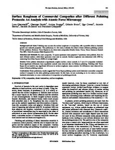
FIG. 1. Example of homogeneous roughness situation in the wind direction sector.
5
Nj
j51 k51
j k
j k
j 0
M
1
2
3
(9) Experimental data are inevitably affected by error. If this was not true, a single measurement in each wind direction sector would be sufficient to estimate the relative z 0 value. Fourth, this is not the case and the y jk is a stochastic process: the expected z 0 value can be deducted from the respective probability density function. A reasonable estimate can be obtained from the median value by sorting in ascending numerical order the values obtained for the y jk variable and finding the 50th percentile [i.e., the median; Press et al. (1992)]. Among other things, this procedure is an indirect method of evaluating the suitability of the wind direction sector divisions. If y jk values are graphed after having executed a dataset sorting, graph results should define a distinct plateau, as can be seen in Fig. 1. If this does not occur, it is probable that the sector under consideration presents an exaggerated high j level of unhomogeneity. Therefore, once the ymed median value is defined, an estimate of surface roughness for the jth sector is obtained from the equation j z 0 5 exp(ymed ).
(8)
This procedure assumes that numerical parameters of the similarity universal function for the wind speed profile are known a priori. The wide range of these parameters found in the literature suggests that it could be interesting to define a workable methodology based on measurements from an ultrasonic anemometer within the surface layer at a fixed station that would permit the simultaneous estimate of surface roughness in each wind direction sector and numerical parameters in the universal function of which only the functional equation (which, as has been seen, is continuous but not derivable in each point of its existing dominion) is known. The method can actually be articulated in the following manner: proceed as previously described in the subdivision of available measurements according to wind direction. The available N measurement is then subdivided in M subsets each with numerousness N j . The selection of wind sectors should be performed based on the characteristics of the ground surface near the measurement points and on the statistical representation of the sectors. In particular, when a sector is characterized by a very low wind frequency in that direction, merging it with a contiguous sector or changing the sector definition in order to have all the N j’s roughly equal should be considered. The quantities to estimate are vector z 0
The difficulties of estimating parameters are twofold. First, the function cannot be reduced to a general linear least squares problem, and second, the function is continuous but not differentiable everywhere. This does not permit the use of techniques requiring the use of partial derivatives with respect to required parameters. Even if the resolution of such optimization problems could be attempted with nondifferential mathematical optimization techniques (Gaudioso 1984), the large number of parameters to be estimated does not recommend the direct resolution. Note that if a direct resolution is desired, it is advisable to adopt numerical methods similar to the downhill simplex method proposed by Murray (1972). This optimization algorithm, described in detail in Press et al. (1992), has the fundamental characteristic of not requiring the calculation of the partial derivatives of the objective function with respect to the parameters for which the optimum value is sought. Basically, the search for the optimum value is performed within the parameter space by analyzing the value assumed by the objective function at the vertex of a hypertetrahedron (known as the ‘‘simplex’’). On the basis of the result obtained in a search, the algorithm modifies the geometrical structure of the search simplex by using one of the following strategies: reflection, reflection and expansion, contraction, and multiple contraction; then a new search is performed. The algorithm is concluded when the estimate of the parameters reaches a substantial equilibrium. A useful and interesting example of the implementation of the algorithm is the AMOEBA routine, part of the well-known mathematical library, Numerical Recipes in FORTRAN (Press et al. 1992), which was used by us in the data processing of these measurements. The easiest and most efficient estimating method is as follows. Step 1: For the three numerical parameters a1 , a 2 , a 3 , a guess value is assigned [e.g., 16, 17, and 0.29, respectively, as often suggested in the literature (van Ulden and Holtslag 1985)]. This way, the only unknowns of the problem are the z 0 vector elements. Step 2: As previously done, surface roughness z 0 length values are determined for any desired sectors, and these constitute the initial guess for estimates. All available data are used in spite of its associated atmospheric stabilities.
MAY 1998
SOZZI ET AL.
Step 3: The N j variables are obtained from standard measurements of a given jth sector, w kj 5 ln
12
z ku kj 2 , z0j (u* ) kj
or, in other words, the realization of the similarity universal function of the wind speed vertical profile at various atmospheric stability situations. Remember that connected with each w ‘‘event,’’ the experimental value of atmospheric stability (z/L) and friction velocity (u*) is known. Step 4: The least squares function,
O O [w 2 C 1Lz , a , a , a 2] , M
F(a1 , a2 , a3 ) 5
2
Nj
j k
j51 k51
M
j k
1
2
3
depends only on three numerical parameters characteristic of C M . An estimate of these parameters is obtained by reducing this function to a minimum. Even if this function is not derivable everywhere, its minimization is more easily reached than that of Eq. (9) due to the limited number of parameters to estimate. The aforementioned routine AMOEBA is utilized for this purpose. Step 5: After obtaining the new estimates for the three numerical parameters of the similarity universal function, the procedure goes to step 2 and terminates when both surface roughness length and the three numerical parameter values reach ‘‘equilibrium’’ values. This procedure is actually equivalent to the direct resolution of the minimization problem (9), even though it is easier to use and verify since it is possible to directly control results obtained step by step. To further decrease computational efforts, it is possible to also partially modify step 3. Instead of considering all w variable values singly, it is possible and advisable to substitute them with respective averages of z/L intervals at a predefined size. This reduces the irregularity of data used in the parameter-estimating process, making it more stable and faster. The synthetic illustration of the operating procedure presents some interesting aspects. 1) It permits the use of ultrasonic anemometer measurements for simultaneous estimation of surface roughness parameter for each wind direction sector and universal similarity function numerical parameters of the wind speed vertical profile. 2) It permits the use of not only the measures obtained in strong wind adiabatic situations but also in every type of stability situation. This usually means that even highly stable and unstable situations can be considered. This permits minimizing campaign duration (as well as relative economical costs) and increasing data statistics upon which this estimating procedure is based. 3) It requires only a low-cost sensor placed at a fixed altitude. This is an iterative procedure and its convergence should be demonstrated before utilization. As it often
465
occurs, even in this case, it is not easy to demonstrate method convergence with strictly mathematical arguments and a practical demonstration based on numerical experiments is the most sensible approach. Some results of the experiment are cited in the next section. However, it can be stated that the iterative procedure converges very quickly; in fact, after two iterations, the surface roughness values are practically stable, while after three or four iterations even numerical parameters of the similarity universal function reach their ‘‘equilibrium’’ value. 3. Use of the methodology in an experimental campaign In an attempt to understand the mechanisms underlying the serious air pollution problems frequently encountered in Mexico City, a number of experiments were carried out in the metropolis from 1992 to 1994. More precisely, in the period 1992–93, a contract (C11CT90-0868) of the Commission of the European Communities (CEC) Directorate General XII (DG XII) permitted the investigation of the micrometeorological characteristics of the area in which the city is located (Valle de Me´xico). The principal goal of the experimental campaign was to organize an Italo-Mexican work group to install micrometeorological monitoring stations and undertake the necessary data processing. In view of the preliminary character of this activity, work was limited to setting up a single measurement station, initially equipped with traditional meteorological instrumentation, and only toward the end of the campaign was an ultrasonic anemometer added. Alongside the fixed instrumentation, radiosoundings were performed for limited time intervals in order to determine the thermal stratification of the PBL. Some of the results obtained are reported in Salcido et al. (1994), and most of the measurements performed are provided in the campaign’s final report (document number E 90042-01-RT) available from DG XII of the CEC. In 1994, the Federal District allocated funds to the Instituto de Investigaciones Electricas and to Servizi Territorio so that it could continue this form of investigative activity, extending it to cover most of the city area. The original objective that would span many years was the development of a model that would realistically describe the main average meteorological parameters and the turbulence throughout the entire Mexico City area; such data were supposed to provide the necessary meteorological input for models of pollutant dispersion. However, the Mexican economic crisis prevented the completion of the project, and the relevant activities were terminated during 1994. The experimental work involved contributions of the Institute of Atmospheric Science of the National Autonomous University of Mexico (UNAM) and the University of Vera Cruz. The experiment was based on four identically equipped meteorological monitoring stations. The sen-
466
JOURNAL OF APPLIED METEOROLOGY
sors present were an RM Young triaxial propeller anemometer, a Vaisala thermohygrometer, a LI-COR pyranometer, a REBS net radiometer, a Vaisala barometer, and a USAT-3 (METEK GmbH) ultrasonic anemometer. On all sensors, except the ultrasonic anemometer, measurement acquisition was performed by a Campbell CR10 datalogger. The ultrasonic anemometer was equipped with an independent acquisition and data-processing system. All measurements recorded were stored in a PC present at the various stations. In addition, for a limited time period, radiosoundings were performed (on average, five per day) to identify the vertical profiles of wind, temperature, and air humidity, correlating them to the turbulent fluxes registered at ground level. Three of the meteorological stations were located within the city (one at the Institute of Atmospheric Science of UNAM), while a fourth was situated in a zone several tens of kilometers northeast of the center of Mexico City, in a locality known as Vaso de Texcoco. Not all of the 1994 campaign results have been published yet, but they are available at the Instituto de Investigaciones Electricas. [Campaign details and results can be found in Salcido et al. (1994).] The present work considers only some of the data relative to the station at Vaso de Texcoco, in particular those of the ultrasonic anemometer in the periods 9–28 June and 8–30 July 1994. In the first place, a description of the measurement site must be taken into account. Vaso de Texcoco lies several tens of kilometers from the center of Mexico City. The terrain is completely flat and composed of bare soil. It lies at a considerable distance where the part of the city closest to the locality is characterized by a very limited vertical extension. At approximately 150–200 m north-northeast from the meteorological station, there were a few scattered low shacks (approximately 3 m high) and to the northnorthwest at approximately 1–1.5 km, there were a few 10-m-high trees. The Vaso de Texcoco station, as well as the other stations, was equipped with conventional instruments and an ultrasonic anemometer (METEK, mod.USAT3, Metek GmbH, Hamburg, Germany), functioning at a sample frequency of 10 Hz. To simplify the data-processing procedure, it was decided to use data-processing hardware and software supplied by the ultrasonic sensor manufacturer, which caused a few restrictions, as explained below. The importance of this station was that it was one of the few sites possible (with available electricity supply) that was not perturbed by the presence of the city. This allowed the acquisition of micrometeorological information, which was virtually unperturbed by the city and thus of certain interest for comparison with the analogous (and simultaneous) measurements performed within the city. Unfortunately, the unreliability of the electrical grid brought about the loss of a significant number of measurements, which accounts for the relatively lim-
VOLUME 37
ited number of data available with respect to the theoretical amount. Data-processing procedures included the following. R Data obtained from the ultrasonic sensor were processed according to Kaimal and Finnigan’s (1994) recommendations with a 10-min averaging time that provided friction velocity, the covariance between vertical velocity and temperature, variance of wind components and temperature, as well as average value of the three wind vector components and temperature. Note that the choice of using sensor manufacturer data processing led to the use of only two system rotations for reference. R Values obtained with 10-min sample time were put together in semihourly values averaging the averages, the variances, and the covariances, while the following equation was used for the friction velocity:
!O 1u* 2 . 2
3
u* 5
(i)
i51
This procedure substantially coincides with Weseley (1988) and de Bruin et al. (1993) and represents a filtering action of low frequency, in agreement with the suggestions of Panofsky and Dutton (1983). R The value of the z/L stability parameter was obtained by using the usual definition in which the average semihourly friction velocity value and the covariance between vertical components of the wind speed and temperature can be found. There were 1244 measurements (semihourly means) taken during the campaign, corresponding to approximately 60% of theoretical data. The incidence of the interruptions of the electricity supply turned out to be very high. Meteorological characteristics encountered were such that no measurement could be classified as extremely convective or stable. This is because during the measurement periods, the situations at high insolation were never accompanied by winds of less than about 2 m s21 . In practice, the variation interval of the stability parameter z/L has an upper limit of about 2 and a lower limit of about 22. Therefore, all data obtained were used during the parametric estimate procedure. The data were initially divided into 36 wind direction sectors at a 108 width starting from the north. Due to the unhomogeneity of the number of data proper to each sector, and the surface homogeneousness of various sectors especially in the south and southwest, these sectors were reduced to 25. Table 1 indicates that both estimates were obtained after the first iteration, as well as final estimates. Note that the surface roughness is greater in the angular sector between north and east, while it is uniformly low in all the other directions. A comparison with the local geographic situation can at least partially explain such results. In effect, the city is located so far away from Texcoco (several tens of kilometers) as to not significantly influence the surface roughness. Also
MAY 1998
467
SOZZI ET AL.
TABLE 1. The z0 values of various wind direction sectors obtained at Vaso de Texcoco with the proposed method from ultrasonic anemometer set at a height of 10 m. Mean direction (8N)
Number of data points
z0, first iteration (m)
z0, final value (m)
Mean direction (8N)
Number of data points
z0, first iteration (m)
z0, final value (m)
5 15 25 35 45 55 65 75 85 95 105 115 125
108 91 108 86 72 49 31 27 24 20 13 16 10
0.200 0.337 0.405 0.390 0.209 0.112 0.169 0.182 0.199 0.091 0.078 0.052 0.084
0.195 0.327 0.389 0.376 0.194 0.111 0.141 0.166 0.179 0.086 0.063 0.047 0.076
135 145 155 165 175 195 230 280 325 335 345 355 —
36 34 49 35 19 24 25 49 34 90 97 97 —
0.114 0.059 0.017 0.018 0.012 0.027 0.033 0.019 0.032 0.034 0.053 0.092 —
0.112 0.059 0.017 0.016 0.010 0.026 0.032 0.018 0.030 0.032 0.048 0.085 —
note that the vertical extension of the buildings (in any case, very far off ) is quickly reduced as one moves farther away from the city’s center. The numerous suburbs of the city, which are not visible from Texcoco, have a vertical elevation of no more than 6 m. The measurement station is cut off from the suburban area by a completely flat, bare plain entirely free of irregularities. As far as the angular sector between north and east is concerned, note that the relatively high surface roughness encountered could be due to a combination of different causes. First is the presence in these directions of orographic irregularities, far off clusters of trees (at a few kilometers distance), and sparse trees at closer distances, as well as the presence of some isolated shacks, standing very near to the measurement point. It is likely that the influence of the shacks is not marginal, although there is no way of knowing their contribution to the overall estimate of the roughness length; this highlights the fact that the determination of z 0 is a rather delicate problem and that a reliable determination, needed, for example, in prognostic PBL models, requires either a longer temporal extension of the measurement campaign or a greater number of measurement points
within the same area in order to minimize the impact of local flux distortions. It would also have been interesting to compare this methodology of parametric estimation with the other methods mentioned. Unfortunately, the unavailability of anemological measurements at several levels and a dataprocessing system unsuitable for a reliable estimation of s u , as requested by Panofsky and Dutton (1983), prevented such comparison. It is therefore impossible to say whether the proposed method is more sensitive than others to the presence of local flux obstructions. Weighing all sectors, an average surface roughness value of 0.152 m is obtained. The median value of sector roughness data is 0.111 m, which is very different from the weighed average value. Results are graphed in Fig. 2. At this point, it was possible to estimate numerical parameter values found in the similarity function of the wind speed vertical profile. Results obtained are indicated in Table 2. The value found for parameter a1 is within the experimental range of other campaigns, as reported by Garrat and Hicks (1990). In regard to parameters a 2 and a 3 , only Beljaars and Holtslag (1991) take into consideration the stability levels reached in this experimental campaign. In view of the functional structure of (7c), it is difficult to state whether or not the results obtained are close to the values reported in the literature. The best way of making this comparison is by using a graph. Figure 3 compares the trends predicted by (7c) with the set of parameters
TABLE 2. Wind profile universal similarity function parameter from ultrasonic anemometer data obtained at height of 10 m at Vaso de Texcoco. Parameter
FIG. 2. Surface roughness from measurements obtained by ultrasonic anemometer at a height of 10 m.
a1 a2 a3
Initial value
Final value
16 17 0.29
22.83 11.72 0.416
468
JOURNAL OF APPLIED METEOROLOGY
FIG. 3. Comparison between the wind profile universal function (PSIpM) reported in the literature for stable situations (solid line) and Vaso de Texcoco results (dotted line).
provided in the literature and that are reported in Table 2. A visual examination of the trends confirms a substantial agreement between the two trends. The comparison between function C M reported in the literature and the semiemperical correlation experimental values was also affected in this case, as shown in Fig. 4, where again it can be noted that dispersioncharacterizing experimental data decreases notably when considering block experimental averages (Fig. 5). In conclusion, the asymptotic equation for the similarity universal function in stable situations is CM
1L2 5 2a a L 5 24.9 L , z
z
2
z
3
which is also very much in accordance with the literature. 4. Conclusions This work has identified an iterative procedure for contemporarily estimating z 0 surface roughness and similarity universal function parameters of the wind speed vertical profile. This procedure is based on measurements obtained from a single ultrasonic anemometer placed at a fixed altitude (within the surface layer) and utilizes practically all measurements obtained in spite
VOLUME 37
FIG. 5. Comparison between wind profile universal similarity function (block averaged) and the semiempirical correlation.
of PBL stability status. The adoption of this procedure could simplify and lessen costs of experimental campaigns for characterizing surface roughness of a site and could also permit the control of this parameter’s evolution due to seasonal changes verified in local vegetation by means of a fixed meteorological station. This procedure was later applied to results obtained at Vaso de Texcoco near Mexico City. The procedure led to the estimate of surface roughness relative to all wind directions, as well as numerical parameters found in the similarity universal function wind speed vertical profile. Results obtained for these parameters were very realistic and in accordance with the existing literature, thus confirming the validity of the method and its application to actual cases. Its algorithmic stability and relative simplicity make it suitable as both a basic processing method of measurements gathered in ad hoc micrometeorological campaigns, as well as an integral part of the data processing of a fixed meteorological station equipped with an ultrasonic anemometer. Since the proposed method is based on measurements at one height only, it is indispensable that the measurement height is always within the surface layer. This means that the height must not be too high, especially in zones experiencing frequent weak winds, where strongly convective situations are consequently highly probable. Apart from this, the normal instructions (EPA 1987) for the installation of a meteorological station are valid, particularly those regarding the minimum distance between the measurement pole and the nearest obstacles. Acknowledgments. The authors would like to express their appreciation to Instituto de Investigaciones Electricas (Morelos, Mexico) that provided the Texcoco data. In particular, we would like to express a special thanks to Ricardo Saldan˜a and Alejandro Salcido (IIE), who carried out and processed the Texcoco data. REFERENCES
FIG. 4. Comparison between wind profile universal similarity function and the semiempirical correlation.
Beljaars, A. C., and A. A. M. Holtslag, 1991: Flux parameterization over land surfaces for atmospheric models. J. Appl. Meteor., 30, 327–341.
MAY 1998
SOZZI ET AL.
Bintanja, R., and M. R. van der Broeke, 1995: Momentum and scalar transfer coefficients over aerodynamically smooth Antarctic surfaces. Bound.-Layer Meteor., 74, 89–111. Brutsaert, W., 1982: Evaporation into the Atmosphere—Theory, History and Applications. D. Reidel, 299 pp. Charnock, H., 1955: Wind stress on a water surface. Quart. J. Roy. Meteor. Soc., 81, 639–640. de Bruin, H. A. R., W. Kohsiek, and B. J. J. M. van den Hurk, 1993: A verification of some methods to determine the fluxes of momentum, sensible heat and water vapor using standard deviation and structure parameter of scalar meteorological quantities. Bound.-Layer Meteor., 63, 231–257. EPA, 1987: On-site meteorological program guidance for regulatory modeling applications. U.S. Environmental Protection Agency Rep. EPA-450/4-87-013, 171 pp. Garratt, J. R., and B. B. Hicks, 1990: Micrometeorological and PBL experiments in Australia. Bound.-Layer Meteor., 50, 11–29. Gaudioso, M., 1984: Metodi di ottimizzazione non differenziabile. Metodi e Algoritmi per L’ottimizzazione, Pitagora, 514 pp. Haenel, H. D., 1993: Surface layer profile evaluation using a generalization of Robinson’s method for the determination of d and z 0 . Bound.-Layer Meteor., 65, 55–67. Kaimal, J. C., and J. J. Finnigan, 1994: Atmospheric Boundary Layer Flows—Their Structure and Measurement. Oxford University Press, 289 pp. Lo, A., 1979: On the determination of the boundary layer parameters
469
using velocity profiles as sole information. Bound.-Layer Meteor., 17, 465–484. Murray, W., 1972: Numerical Methods for Unconstrained Optimization. Academic Press, 144 pp. Nieuwstadt, F. T. M., 1978: The computation of the friction velocity and the scale temperature from temperature and wind velocity profiles by least squares methods. Bound.-Layer Meteor., 14, 235–246. Panofsky, H. A., and J. A. Dutton, 1983: Atmospheric Turbulence: Models and Methods for Engineering Applications. Wiley and Sons, 397 pp. Press, W. H., B. P. Flannery, S. A. Teukolsky, and W. T. Vetterling, 1992: Numerical Recipes in FORTRAN—the Art of Scientific Computing. Cambridge University Press, 963 pp. Salcido, V. A., R. Saldana, R. Sozzi, and D. Fraternali, 1994: Estudio de la Micrometeorologia del Valle de Mexico Informe Final (in Spanish). Instituto de Investigaciones Electricas, 327 pp. Sorbjan, Z., 1989: Structure of the Atmospheric Boundary Layer. Prentice-Hall, 317 pp. Stull, R., 1988: An Introduction to Boundary Layer Meteorology. Kluwer Press, 666 pp. van Ulden, A. P., and A. A. M. Holtslag, 1985: Estimation of atmospheric boundary layer parameters for diffusion applications. J. Appl. Meteor., 24, 1196–1207. Wesely, M. L., 1988: Use of variance techniques to measure dry air– surface exchange rates. Bound.-Layer Meteor., 44, 13–31. Wieringa, J., 1993: Representative roughness parameters for homogeneous terrain. Bound.-Layer Meteor., 63, 323–363.