The commercial classified information of components is protected. ... "black box" that has to provide only the strictly determined set of information via its ...
Modelling and Simulation of Multibodies in Mechatronic Systems
R. Kasper, D. Vlasenko Otto-von-Guericke-University Institute of Mobile Systems (IMS)
Abstract. This paper presents the detailed description of the method for the component-oriented modelling and simulation of mechanical parts of mechatronical systems, implemented in the mechatronic simulation software Virtual Systems Designer (VSD). The simulation of complex mechatronic systems shows the stability and efficiency of the proposed approach.
1
Introduction
The implementation of the component-oriented in simulation tools significantly reduces the cost and development time, increasing the software usability. All popular simulation tools used today support componentoriented development of models, where mechanical systems are considered as a hierarchy of components, where components usually include bodies, joints, external forces, etc. But this type of modularization in most cases is given up during simulation, especially for mechanical systems, because common modelling formulations use access to the complete system. On the other hand, there are big advantages of a simulation on the basis of components: • Components can be modelled, tested and compiled. Then they can be used in a way similar to software components that encapsulate their internal structure and can be connected via interfaces. • The commercial classified information of components is protected. A component works like a "black box" that has to provide only the strictly determined set of information via its interfaces. The components's internal data: parameters of constraints, forces, masses of internal bodies, etc. are unknown to the users of components. • Critical effects like coulomb friction, backslash etc. can be encapsulated inside a subsystem. • The tool can be easily integrated into more general tools for the development of virtual reality of mechatronic systems. Mechanical objects like bodies, springs, torques, etc. can be used as parents of mechatronic objects. This paper presents Virtual Systems Designer (VSD) for the development of virtual reality of mechatronic systems. The tool is based on the fast component-oriented simulation method, whose time complexity is comparable with the fastest available parallel algorithms. Starting from the extended 3D-CAD model of a mechatronic system, VSD analyses the model’s mechanical properties and the hierarchy of components. Then for each CAD component, defined by design engineers during the model’s development, the correspondent VSD component is generated. The simplification of equations of motion of components in VSD is made by Maple preprocessing module.
2
Description of Component-Oriented Simulation Method
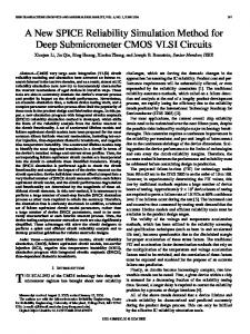
The base idea of the method, shown in Fig. 1, is to perform the simulation of mechanical systems using the hierarchy of submodels that builds up the complete system.
q(tk ), v (tk ) Calculation accelerations v� (tk )
q� (tk +1 ), v� (tk +1 )
Integration
Stabilisation
q(tk +1 ), v (tk +1 ) Figure 1: Simulation steps
of
Components of the first level in general consist of connected bodies. Components of next levels (called children) consist, without loss of generality, of connected submodels (called parents). Since the main number of calculations proceeds inside of components, it follows that the simulation can be distributed easily on several processors. During the simulation on each time step the following tasks have to be performed: 1. Distributed calculation of the absolute accelerations v� (t k ) . 2. Calculation of the absolute coordinates and velocities at the next time step. Using a favorite ODE integration scheme (e.g. Runge-Kutta or some multistep method), the value of the absolute coordinates ~ (t ) and velocities ~ q v (t k +1 ) at the new time step can be obtained. k +1 3. Distributed stabilization of the absolute coordinates q(tk+1) and velocities v(tk+1).
3
Distributed calculation of acceleration
Let be a vector of absolute coordinates of bodies in the simulated mechanical system, … consisting on bodies position coordinates and Euler parameters. Let be the vector of constraints, describing
(
)
T
the joints between bodies, and gb (q) = g1b , … gbn
be the vector of additional constraints on the Euler
parameters 1
g
(1)
where are Euler parameters of the i-th body. The index-one system of differential-algebraical equations then can be written as =T( )v ( ) ( )
( )
(2) ,
·
(3)
,
where v is the vector of absolute velocities, consisting on bodies linear and angular velocities ( ) is the mass matrix , is the vector of external forces (other than constrain forces) ( ) is the constraint Jacobian matrix ( )= T
λ is the vector of Lagrange multipliers. q, v
S1,1
S1,2
S2,1
S2,2
D(1,1) R(1,1)
D(1,2) R(1,2)
D(2,1) R(2,1)
D(2,2) R(2,2) S2
S1 D(1) R(1)
D(2) R(2) S
Q
Q(2)
(1)
S2
S1
Q(1,1)
Q(1,2)
S1,1
S1,2
Q(2,1) S2,1
v� Figure 2: Calculation of acceleration steps
Q(2,2) S2,2
Starting from (3), we can distribute the process of the calculation of accelerations
as it shown in Fig. 2.
3.1 Hierarchical generations of equations of motion Each component gets from its parents their dependency matrices D(i) and R(i):
v� (ei ) = D( i ) Q( i ) + R ( i )
(4)
where v� (ei ) is the vector of accelerations of the i-th parent’s bordering bodies Q( i ) is the vector of forces acting in the i-th parent’s external links. For example, in Fig. 2 the component S1 gets matrices D(1,1), R(1,1), D(2,1), R(2,1) from its parents S1,1, S1,2 etc. Here a body is called bordering to a component, if it has constraints in the component and is connected with external joints. A body is called internal to a component, if it has constraints in the component and is not connected to any external joint. The component generates matrices D and R using the equation of constraints connecting the parents. Here D and R are the dependency matrices:
v� e = DQ + R
(5)
where v� e is the vector of accelerations of component’s bordering bodies Q is the vector of forces in component’s external links. Then the component transmits D and R to its child.
3.2 Calculation of absolute accelerations on the top of hierarchy The component of the highest level calculates Q(i) for each parent i and transmits it to the parent (e.g. in Fig. 2 the component S transmits Q(1), Q(2) to its parents S1, S2 correspondingly).
3.3 Backward hierarchical calculation of absolute accelerations Subsequently, each component gets the current value of Q from its child (e.g. in Fig. 2 the component S1,2 gets Q(2) from its child S1). Using Q the component calculates v� e . Then for each parent i the component calculates Q(i) and transmits it to the parent. Finally the absolute accelerations of all bodies are obtained.
4
Algorithm of distributed post-stabilization
Using standard explicit solver (Runge-Kutta, etc.), the values of coordinates q� (tk +1 ) on the new time step are obtained. However, q� (tk +1 ) do not fulfil nor the equations of joint constraints , nor the vector of additional constraints on the Euler parameters . The drift of constraints grows with time t – at worst quadratically. To overcome this difficulty, the coordinates and velocities can be projected back onto the manifolds given by and ( ). In [4, 5] it was shown that this projection can be done in the successive way. On the first stage for each body i we project its coordinates q� i onto the manifold, given by (1):
( ) ( )
1 i g b q� s 2 gbi q� i + 1 i
q i = q� i −
(
where s i = 0 0 0 e0i
e1i
e2i
e3i
)
T
i
(6)
. On the second step we calculate the stabilized values of coordinates
q as the projection of q on the manifold, given by by : q = q + T(q) ⋅ δ
(7)
where the stabilizing displacement δ is obtained by solving the following minimization problem δ
Z
→ min
with g(q + T(q ) ⋅ δ) = 0
(8)
Depending on the method of projection (orthogonal or energy), the norm δ or δ
Z
Z
can be calculated as δ
Z
= δT δ
= δT Mδ , correspondently.
The distribution of projection of coordinates is similar to the distribution of calculation of accelerations [7, 5]. ˆ (q ) ⋅ v = 0 is also needed. In sake of simulation robustness, the stabilization of velocity constraints g� (q, v ) = G This can be made by the distributed projection of velocities v� on the manifold, given by g� in the manner, similar to the projection of coordinates [7, 5].
5
Implementation
The implementation of method was made in the Virtual System Designer (VSD) software, integrated with a CAD tool Autodesk Inventor. Starting from the hierarchy of component, defined by design engeniers in Autodesk Inventor, VSD generates correspondent objects, describing the components dynamics. During the implementation of the method we needed to solve the problem of rank-deficiency of constraint Jacobian matrix . Commonly, the rank deficiency can be two types: 1. Permanent rank deficiency because of existence of redundant constraints, defined during the modeling. In many cases design engineers develop CAD models using the greater number of constraints than it is needful from the mechanical point of view. For example, stiff connection between two bodies is usually defined as the combination of three plane-to-plane joints, that leads to appeareance three redundant constraints in the vector g . The best way to solve this problem is to elliminate dependent rows from , using the singular value decomposition (SVD) of [3]. Singular configuration. If equations of motion of a complex multibody systems are made in absolute coordinates, the appeareance of singular configuration is very common. This leads to the rank-defitient problems during the simulation of system dynamics. The calulation of accelerations and of stabilizing displacements on the coordinate and on the velocity levels needs the decomposition of the same coordinate-dependent sparse matrix A for the calculation of X 2.
AT AX = B
(9)
where B varies for different types of calculation. In common case columns of A can be linear dependent, therefore, the numericall expensive SVD of A is needed for the calculation of the minimal-norm solution of (9). Nethertheless, in practice X can be calculated as a basic solution of (9). Therefore, we need only to calculate the the numerically cheap QR-decomposition with pivoting AΠ = QR [3, 1]. Since using absolute coordinates, the matrix A usually has a sparse structure and includes both numerical and symbolic elements, e.g. the elements that are constant during the simulation and elements, depending on the coordinates of bodies. We have developed in Maple a preprocessing module, which generates for each component a corresponding Dynamically Linked Llibrary (.dll), decomosing the component’s matrix A [6]. The symbolic simplification of decompositions has several advantages in comparison with standard sparse solvers: • Sparse structure of matrices is used completely without any run time overhead. • The numerical operations with numerical elements of matrices are performed already during the translation. • Additional operations with arrays of indexes (like in usual sparse solvers) are not needed.
6
Robot example
In order to test our software we performed the number of simulations of complex mechatronic systems. In this article we present the simulation of dynamics of the Autodesk Inventor model of the industrial robot SPBot [2]. This is a two-axis robot, equipped with two DC servo motors, for rotating and transferring car engine block. The complete mechanical Autodesk Inventor model consists of 247 parts coupled in several components, shown in Fig 3: upper arm, motors, cyclo-drive gearboxes, etc. The mechanical part of the correspondent VSD model includes 17 bodies connected by 32 joints. Some of model constraints are redundant because of the model’s design in Autodesk Inventor (e.g. the definition of stiff connection as three plane-to-plane joints leads to the generation of three redundant constraints). The list of components’ parts is shown in Table 1.
Figure 3: Hierarchy of components of SPBot robot model
Name component Vertical Motor
Parts Rotor, Housing
Horizontal Motor
Rotor, Housing
Vertical Cyclo-Drive Gearbox Horisontal CycloDrive Gearbox Complete Model
High-speed Shaft, Slow-Speed Shaft, 2 Cycloid Discs, Housing High-speed Shaft, Slow-Speed Shaft, 2 Cycloid Discs, Housing Vertical Motor, Horizontal Motor, Vertical Gearbox, Horisontal Gearbox, Base, Lower Arm, Upper Arm
Joints, External Forces, Sensors 1 Revolute Joint, Driving Torque, Velocity Sensor 1 Revolute Joint, Driving Torque, Velocity Sensor 4 Revolute Joints, 3 Gear Constraints 4 Revolute Joints, 3 Gear Constraints 4 Revolute Joints, 6 Plane Joints, 6 Cylindrical Joints
Table 1: Components of SPBot robot model The simulation data shows that the consequent distributed stabilization algorithm is stable and the model's drift is constant. The component-oriented distribution of calculations together with the implementation of the preprocessing module greatly reduces numerical costs of the simulation. The computations of accelerations and
stabilizing displacements were distributed on the four cores of the Intel Core i7 I7-920 Quad Core Processor, that significantly reduced the simulation time. The component-oriented approach allows easily develop and simulate electro-mechanical models of motors and integrate them with electrical components of the robot model.
7
Conclusion
The implementation of the component-oriented approach for the modelling and simulation of dynamics of mechanical parts of mechatronic systems significantly simplifies the development, test and reuse of models. The distribution of calculations on the base of components together with the implementation of the preprocessing module for the simplification of components’ equations of motion greatly reduces numerical costs of the simulation. The example of SPBot robot mechatronical model illustrates the implementation of the proposed method. References [1] Å. Björck. Numerical Methods for Least Squares Problems. SIAM, Philadelphia, 1995 [2] M.M. Dalvand (2009): Automation of a complex transfer operation using a polar manipulator. Assembly Automation, Vol. 29, No. 1., pp. 68-74. [3] Golub G.H., Van Loan Ch.F. Matrix Computations, The John Hopkins University Press, Baltimore and London, 1989, Second Edition. [4] D. Vlasenko, R. Kasper (2009): Implementation of consequent stabilization method for simulation of multibodies described in absolute coordinates Multibody System Dynamics (accepted, to appear). [5] D. Vlasenko, R. Kasper (2009): Successive projection method for the simulation of spatial dynamics of multibodies. Proceedings of Multibody Dynamics 2009 (ECCOMAS Thematic Conference), Warsaw, Poland, June 29-2 July, 2009 [6] D. Vlasenko, R. Kasper (2008): Implementation of the Symbolic Simplification for the Calculation of Accelerations of Multibodies. Proceedings of Industrial Simulation Conference 2008, Lyon, France, 911 June, 2008. [7] D. Vlasenko, R. Kasper (2007): Integration Method of CAD Systems. Proceedings of the ASME 2007 International Design Engineering Technical Conferences & Computers and Information in Engineering Conference IDETC/CIE 2007 September 4-7, 2007, Las Vegas, Nevada, USA.