Method of Fault Isolation in Electrical Circuits Alexey Zhirabok
Daniil Tkachev
Department of Radio and Electronics Far Eastern State Technical University Vladivostok, Russia
[email protected]
Department of Radio and Electronics Far Eastern State Technical University Vladivostok, Russia
[email protected]
Abstract— The problem of fault diagnosis in electrical circuits is studied. The suggested method is based on diagnostic observers. The procedure of observer synthesis for circuits described by linear equations is developed. The existence conditions to design the observer invariant with respect to the fault are considered. The example of electrical circuit and simulation results are given.
structure of the circuit and values of the resistors, capacitors, and inductances, H is a constant matrix describing measurements. Vector equation (1) can be obtained on the basis of the equations
C U (t ) = I (t ) , LI (t ) = U (t )
I. INTRODUCTION Electrical circuits are of importance both on their own and a convenient tool for modeling different technical objects such as transformers, synchronous and asynchronous electrical machines, drives, and so on. For this reason, electrical circuits are the subject of investigation for fault diagnosis. The majority of papers considering the problem of fault diagnosis in electrical circuits use methods of identification as usual (see, e.g. [1-4]). These methods allow providing an exhaustive analysis (in particular, determining values of parameters) but demand comprehensive information about the circuit operation and are of high computational complexity. At the same time, in practice, one need only to know that some parameters have been changed. In this paper, the method of fault isolation in electrical circuits described by linear equations is suggested. It does not use methods of identification and allows finding out a parameter which has been changed, i.e. has been deviated from its nominal value. It is assumed that the circuit contains resistors, capacitors, inductances, sources and may operate in no stationary regime. The method is based on the following general description of the circuit:
x(t ) = Fx(t ) + Gu (t ) , y (t ) = Hx(t ) ,
(1)
where x(t ) is the state vector whose components are voltages across the capacitors and currents through the resistors and inductances, u (t ) is the vector whose components are values of the sources, y (t ) represents measured components of the state vector; F and G are constant matrices describing a
978-1-4244-7826-2/10/$26.00 ©2010 IEEE
308
and Kirchhoff’s lows. We will consider as an example the electrical circuit shown in Fig. 1. Kirchhoff’s lows describing the circuit are as follows: I1 = I 2 + I 5 , I1 = I 3 + I 4 , R1 I 5 + U 1 + U 3 = E , R2 I 2 + U 1 + U 2 + U 3 = E , − R3 I 4 + U 3 = E . Using the equations
C1U 1 (t ) = I 1 (t ) ,
C 2U 2 (t ) = I 2 (t ) ,
C3U 3 (t ) = I 3 (t ) and assuming that ⎛ U1 ⎞ ⎜ ⎟ x = ⎜U 2 ⎟ , ⎜U ⎟ ⎝ 3⎠
⎛U ⎞ y = ⎜⎜ 1 ⎟⎟ , ⎝U 2 ⎠
one obtains the following matrices in the model (1): ⎛ k1 + k 2 ⎜ F = ⎜ k3 ⎜k + k 5 ⎝ 4
k1 k3 k4
k1 + k 2 ⎞ ⎟ k3 ⎟, k 4 + k 5 + k 6 ⎟⎠
ΦF = F*Φ + J *H ,
I5
R1
→
RH = H *Φ ,
С2 I2
It is known [6] that the observer can be designed in canonical form when
С3
С1
I4 ↓
I3 ↓
I1 ↑
⎛0 1 0 ⎜ ⎜0 0 1 F* = ⎜ ⎜ ⎜0 0 0 ⎝
E
Figure 1. Electrical circuit
⎛ − (k1 + k 2 ) ⎞ ⎜ ⎟ G=⎜ − k3 ⎟, ⎜ − (k + k + k ) ⎟ 4 5 6 ⎠ ⎝
(3)
G* = Φ G . R3
R2
→
.
0⎞ ⎟ 0⎟ ⎟, ⎟ 0 ⎟⎠
H * = (1 0 … 0 ) .
⎛1 0 0⎞ ⎟⎟ , H = ⎜⎜ ⎝ 0 1 0⎠
(4)
It can be shown that the first equation in (3) for canonical form (4) takes the form
where
Φ 1 = RH ,
k1 = −
1 , C1R2
k2 = −
1 k4 = − , C3 R2
1 , C1R1
k3 = −
1 k5 = − , C3 R1
1 , C 2 R2
Φ i +1 = Φ i F − J i H , i = 1,2,..., k − 1 ,
Φk F = Jk H ,
1 k6 = − . C 3 R3
where k is a dimension of the observer. These equations can be transformed into the single one
Assume that a fault is a deviation of resistance (for resistors) or capacity (for capacitors) from its nominal value. The problem is to design tools for fault detection and isolation. II. PROBLEM SOLUTION General relationships To detect and isolate faults, so-called observers are used. The observer O is described by the following equations:
A.
x* (t ) = F* x* (t ) + G* u (t ) + Jy (t ) + Kr (t ) , y* (t ) = H * x* (t ) ,
(2)
where x* (t ) is the observer state vector, y* (t ) is the output, F* , G , J , H * , and K are constant matrices, r (t ) is the residual. It is assumed that if there are no faults, the equality
RHF k = J 1 HF k −1 + J 2 HF k −2 + … + J k H .
(6)
This equation is a basis to find a minimal dimension of the observer and the matrices J 1 , J 2 ,… , J k which are used for obtaining the rows of the matrix Φ from (5). If this matrix satisfies the condition Φ = NM for the matrix M specified below and some matrix N , then the matrix G* = ΦG is obtained. Otherwise one has to find another solution to equation (6). As a result, the observer invariant with respect to the considered fault has been built. The observer O is sensitive to some set S of faults: if the fault d from this set occurs, then the residual r (t ) becomes nonzero; if d ∉ S , then r (t ) = 0 and the observer is said to be invariant with respect to the fault d . To isolate the faults, one has to use a bank of the observers {O1 , O2 ,..., O p }
r (t ) = Ry (t ) − y* (t ) = 0
corresponding to the sets
holds, r (t ) ≠ 0 otherwise; here R is some matrix.
{S1 , S 2 ,..., S p } .
Assume that the matrix Φ exists such that
x* (t ) = Φx(t )
(5)
If d i , d j ∈ S q for all q , then the faults d i , d j
∀t
in the unfaulty case. It is known [5] that matrices describing the circuit and observer satisfy the equations
309
are
indistinguishable, or equivalent. In our case, the faults d1 ÷ d 6 correspond to the capacitors C1 ÷ C 3 and the resistors R1 ÷ R3 , respectively.
B. The fault d1 . Main relations To be specific, consider the fault d1 corresponding to the capacitor C1 . To design the observer invariant with respect to the fault d1 , introduce the matrix M 1 with maximal number of linearly independent rows such that (∂ / ∂C1 ) M 1 ( Fx + Gu ) = 0 .
⎛ 0 1 0⎞ ⎟⎟ . It can be shown In our case one obtains M 1 = ⎜⎜ ⎝0 0 1⎠ that the observer will be invariant with respect to the fault d1 if Φ = N1 M 1 for some matrix N1 .
If these inequalities do not hold, the observer invariant with respect to the fault d1 can not be built. It is easily to check that in our case the inequalities hold. C. The fault d1 . Solution Consider the fault d1 with R = (0 1) . In this case equation (6) is solvable only for k = 2 and (0 1) HF 2 = ( K1 K 2 K 3 ) = H1Fk3 + H 2 F ( k3 + k4 + k5 + k6 ) − H1k3k6 − H 2 k3 ( k5 + k6 )
where
K1 = (k1 + k 2 )k 3 + k 32 + (k 4 + k 5 )k 3 ,
The condition Φ = N1 M 1 and the second equation in (3) result in the equality RH = H * N1 M 1 . It can be rewritten in the form
(R
⎛H ⎞ ⎟⎟ = 0 . − H * N1 )⎜⎜ ⎝ M1 ⎠
(7)
K 2 = k1k3 + k32 + k 4 k3 , K 3 = (k1 + k2 )k3 + k32 + k3 (k 4 + k5 + k6 ) .
This equation results in J 1 = (k 3
This equation has nontrivial (when R ≠ 0 ) solution if rows of the matrices H and M 1 are linearly dependent. This is equivalent to the inequality
J 2 = (− k 3 k 6
(k3
If this condition does not hold, the observer invariant with respect to the fault d1 does not exist. In our case this condition holds, and a solution to equation (7) is R = (0 1) .
Φ 2 = Φ1F − J1H =
k3
k3 ) − (k3
(0
k3 + k 4 + k 5 + k 6
− ( k 4 + k5 + k6 ) k3 ),
0) =
(8)
⎛− k ⎞ G* = ΦG = ⎜⎜ 3 ⎟⎟ . ⎝ 0 ⎠ One can check that the condition Φ = N1 M 1 holds for some matrix N 1 therefore the observer O1 invariant with respect to the fault d 1 has been built. It can be shown that the matrix
N 1 M 1 F = F* N1 M 1 + J * H that is equivalent to the relation N1 M 1 F = ( F* N1
−k 3 (k 5 + k 6 ) ) ,
Φ 1 = RH = (0 1 0) ,
⎛H ⎞ ⎟⎟ < rank ( H ) + rank ( M 1 ) . rank ⎜⎜ ⎝ M1 ⎠
Rewrite the first equation in (3) in the form
k3 + k 4 + k5 + k6 ) ,
⎛ − 2⎞ K = ⎜⎜ ⎟⎟ ensures a stability of the observer. ⎝ −1⎠
⎛M ⎞ J * )⎜⎜ 1 ⎟⎟ . ⎝H ⎠
It should be noted that the capacitor C1 connects with the coefficients k1 and k2 . It follows from equations (8) that they do not contain k1 and k2 . This corresponds to the fact that the observer O1 is invariant with respect to the fault d 1 . It follows from (8) also that these equations contain other coefficients k 3 ÷ k 6 therefore the observer O1 is sensitive to other faults, i.e. S1 = {d 2 , d3 , d 4 , d5 , d6 }.
Criteria of solving this equation are as follows:
⎛ M1 ⎞ ⎟ ⎜ ⎛M ⎞ rank ⎜ H ⎟ < rank ( M 1 F ) + rank ⎜⎜ 1 ⎟⎟ , ⎝ H ⎠ ⎜M F ⎟ ⎝ 1 ⎠
D. The faults d 2 , d 3 , and d 5
⎛M F ⎞ rank ⎜⎜ 1 ⎟⎟ < rank ( M 1 F ) + rank ( M 1 ) . ⎝ M1 ⎠
d2
310
Obtain the observer O2 invariant with respect to the fault corresponding to the capacitor C2 . In this case one
⎛1 0 0⎞ ⎟⎟ . It can be shown that if one let obtains M 2 = ⎜⎜ ⎝0 0 1⎠ R = (1 0 ) , then equation (6) reduces to
⎛ 1 J1 = ⎜⎜ C1 ( k6 + k5 ) − R 1 ⎝ ⎛k J 2 = ⎜⎜ 6 ⎝ R1
(1 0) HF 2 = H1F ( k1 + k2 + k4 + k5 + k6 ) + H 2 Fk1 − H1 ( k1 + k2 ) k6 +
Φ 1 = RH = (C1
This equation results in the following matrices:
k 2 k 4 − k1 ( k5 + k 6 )) ,
Φ 1 = (1 0 0 ) , 0
k1 + k2 ) ,
The condition Φ = N 2 M 2 holds for some matrix N 2 therefore the observer invariant with respect to the fault d 2 has been built. Obtain the observer O3 invariant with respect to the fault d 3 corresponding to the capacitor C 3 . One can obtain
⎛1 0 0⎞ ⎟⎟ in this case. Notice that because M 3 = ⎜⎜ ⎝0 1 0⎠ ⎛1 0 0⎞ ⎟⎟ , the faults d 3 and d 6 are equivalent and M 6 = ⎜⎜ ⎝0 1 0⎠ indistinguishable. It can be shown that R = (k3 − ( k1 + k2 ) ) according to (7) and (6) reduces to
It can be shown by analogy with the observer O1 that S2 = {d1, d3 , d 4 , d5 , d6} , S3 = {d1, d 2 , d 4 , d5} , S4 = {d1, d 2 , d 3 , d 4 , d 6 }. The relations between the observers and faults can be represented by a table (Table 1). An analysis shows that the observer invariant with respect to the fault d 4 can not be built but this fault can be isolated that follows from Table 1. III. SIMULATION RESULTS
− ( k1 + k2 ) )HF = − H 2 k2 k3 ,
For simulating, numerical values of the parameters are as follows: R1 ÷ R3 = 10 Ohm, C1 ÷ C3 = 10−6 F, E = sin(105 t ) .
therefore k = 1, Φ 1 = RH = (k 3
0) ,
One can check that the condition Φ = N 5 M 5 holds for some matrix N5 therefore the observer invariant with respect to the fault d 5 has been built.
⎛ − (k1 + k2 ) ⎞ ⎟⎟ . G* = ΦG = ⎜⎜ 0 ⎝ ⎠
(k3
−C 2
⎛ 1 ⎞ Φ 2 = ⎜⎜ − C1 ( k6 + k5 ) C2 k6 − ⎟⎟ , R1 ⎠ ⎝ ⎛ 1 ⎞ ⎜ ⎟ G* = ΦG = ⎜ R1 ⎟ . ⎜ 0⎟ ⎝ ⎠
J1 = ( k1 + k 2 + k 4 + k5 + k6 k1 ) ,
Φ 2 = ( − ( k 4 + k5 + k 6 )
⎞ 0 ⎟⎟ . ⎠
Equations (5) give:
H 2 ( k2k4 − k1 ( k5 + k6 )).
J 2 = ( − ( k1 + k 2 ) k 6
⎞ − C2k6 ⎟⎟ , ⎠
Fig. 2 illustrates the observer O1 residual behavior. The fault d 2 is modeled by changing the parameter C2 from
−(k1 + k 2 ) 0) ,
J1 = ( 0 − k 2 k3 ) ,
10 −6 F to 2 ⋅ 10−6 F at once at t = 10−3 c. It is obviously that the residual is sensitive to this fault.
G* = 0 .
Because the equality Φ = N 3 M 3 holds for some matrix N 3 , the observer invariant with respect to the faults d 3 and d 6 has been built. Obtain the observer O4 invariant with respect to the fault d 5 corresponding to the resistor R 2 . In this case one can 0 ⎞ ⎛ C − C2 ⎟ . Solutions to equations (7) obtain M 5 = ⎜⎜ 1 0 − C3 ⎟⎠ ⎝ C1 and (6) are, respectively, R = (C1 − C2 ) and
311
TABLE 1. CORRESPONDENCES BETWEEN OBSERVERS AND FAULTS
O1 O2 O3 O4
d1 d 2 0 1 1 0 1 1 1
d3 1 1 0
d4 1 1 1
d5 1 1 1
d6 1 1 0
1 1 1 0 1
IV. CONCLUSIONS
Figure 2. Behavior of the observer
The paper is devoted to the problem of fault diagnosis in electrical circuits. The advantage of the suggested method is that is of small computational complexity in contrast with the known methods of fault diagnosis based on identification; the disadvantage is that it does not allow estimating values of parameters, it allows one only finding parameters which have been changed. Using so-called logic-dynamic approach [6, 7], one can solve the fault diagnosis problem in nonlinear circuits (including non-differential nonlinearities) by linear methods considered in this paper with additional restrictions.
O1 residual
Robustness of the proposed method with respect to the inaccuracies of the electrical components can be achieved by using the known methods based on singular value decomposition and adaptive threshold [5]. ACKNOWLEDGMENT The publication is supported by Russian Foundation of Basic Researches, grants 10-08-00133 and 10-08-91220-СТ. REFERENCES
Figure 3. Behavior of the observer
[1]
O4 residual
Fig. 3 illustrates the observer O4 residual behavior. The fault d 2 is modeled by changing the parameter C2 from 10 −6 F to 2 ⋅ 10−6 F at once at t = 10−3 c. One can see that the residual is sensitive to this fault but its sensitivity is far less than that above because resistance of the capacitor C2 is far less than that of the resistor R2 (see Fig. 1).
[2] [3] [4] [5]
[6]
[7]
312
N. Kinsht, G. Gerasimova and M. Kats, Diagnosis of electrical circuits. Moscow: Energoatomizdat, 1983 (in Russian). J. Benlder and A. Salama, “Fault duagnosis in analog curcits”, Proc. of the IEEE, vol. 73, pp. 35-87, August 1985. P. Butyrin and M. Alpatov, “Continuous diagnosis of tensfomers”, Electricity, pp.46-55, July 1998 (in Russian). A. Alpatova, A. Butyrin and M. Alpatov, “Identification of transformers”, Power ingenering, pp.93-98, April 2001 (in Russian). P. Frank, “Fault diagnosis in dynamic systems using analytical and knowledge-based redundancy – A survey and some new results”, Automatica, vol. 26, pp.459-474, March 1990. A. Zhirabok and S. Usoltsev, “Fault diagnosis for nonlinear dynamic systems via linear methods”, CD ROM Proceedings of the 15th World Congress IFAC, Spain, Barcelona, 2002. A. Zhirabok, “Nonlinear parity relation: logic-dynamic approach.”, Automation and remote control, no 6, pp. 1051-1064, June 2008.