Dec 12, 1999 - Guaranteed frame rate (GFR) service has been attract- ing attention as .... can process an Explicit Rate field in an RM cell; there- fore, they can ...
IEICE TRANS. COMMUN., VOL.E82–B, NO.12 DECEMBER 1999
2081
PAPER
Method of Implementing GFR Service in Large-Scale Networks Using ABR Control Mechanism and Its Performance Analysis Ryoichi KAWAHARA† , Yuki KAMADO†† , Masaaki OMOTANI†† , and Shunsaku NAGATA††† , Members
SUMMARY This paper proposes implementing guaranteed frame rate (GFR) service using the available bit rate (ABR) control mechanism in large-scale networks. GFR is being standardized as a new ATM service category to provide a minimum cell rate (MCR) guarantee to each virtual channel (VC) at the frame level. Although ABR also can support MCR, a source must adjust its cell emission rate according to the network congestion indication. In contrast, GFR service is intended for users who are not equipped to comply with the source behavior rules required by ABR. It is expected that many existing users will fall into this category. As one implementation of GFR, weighted round robin (WRR) with per-VC queueing at each switch is well known. However, WRR is hard to implement in a switch supporting a large number of VCs because it needs to determine in one cell time which VC queue should be served. In addition, it may result in ineffective bandwidth utilization at the network level because its control mechanism is closed at the node level. On the other hand, progress in ABR service standardization has led to the development of some ABR control algorithms that can handle a large number of connections. Thus, we propose implementing GFR using an already developed ABR control mechanism that can cope with many connections. It consists of an explicit rate (ER) control mechanism and a virtual source/virtual destination (VS/VD) mechanism. Allocating VSs/VDs to edge switches and ER control to backbone switches enables us to apply ABR control up to the entrance of a network, which results in effective bandwidth utilization at the network level. Our method also makes it possible to share resources between GFR and ABR connections, which decreases the link cost. Through simulation analysis, we show that our method can work better than WRR under various traffic conditions. key words: ATM, GFR, ABR, large-scale networks, VS/VD, explicit rate control, WRR
1.
Introduction
Guaranteed frame rate (GFR) service has been attracting attention as a new asynchronous transfer mode (ATM) service category. It is intended for users who are either unable to specify traffic parameters needed to request most ATM services, or not equipped to comply with the source behavior rules required by existManuscript received February 16, 1999. Manuscript revised June 21, 1999. † The author is with NTT Information Sharing Platform Laboratories, Musashino-shi, 180-8585 Japan. †† The authors are with NTT Network Service Systems Laboratories, Musashino-shi, 180-8585 Japan. ††† The author is with NTT Phoenix Communications Network, Inc., Tokyo, 100-0004 Japan.
ing ATM services. Traffic parameters for most existing applications cannot be predicted; however, to achieve good throughput, certain cell-loss requirements must be met. For these applications, a static allocation of bandwidth, such as a constant bit rate (CBR) or variable bit rate (VBR), would be inadequate or wasteful because their traffic characteristics are unpredictable. In available bit rate (ABR) service, on the other hand, bandwidth is not allocated statically. Instead, the peak cell rate (PCR) and minimum cell rate (MCR) are specified at call set-up, and the cell emission rate of each virtual channel (VC) is controlled between the PCR and MCR based on feedback from the network. This feedback control makes it possible to utilize the bandwidth effectively without cell loss when the traffic characteristics of the cell stream are unpredictable. However, a source must adjust its cell emission rate according to the network indication. Thus, GFR is being standardized as a new service to provide an MCR guarantee to VCs at the frame level, while allowing the user to send in excess of the MCR. The excess traffic will be delivered on the basis of available network resources. That is, a user can always attain MCR throughput, and may be able to achieve higher throughput if the network is underloaded; this results in effective bandwidth utilization. The performance of various GFR implementations has been studied (e.g., [1]–[4]). These results showed that weighted round robin (WRR) with per-VC queueing at each switch had the best performance. However, WRR is hard to implement in a switch supporting a large number of VCs because it needs to determine in one cell time which VC queue should be served. In addition, it may cause ineffective bandwidth utilization at the network level because its control mechanism is closed at each node without taking account of other node conditions in the network. On the other hand, accompanied with standardization of ABR service, several kinds of ABR control algorithms have been developed, and some of these can handle a large number of VCs. Thus, in this paper, we propose implementing GFR using an already developed ABR control mechanism, which consists of virtual source/virtual destination (VS/VD) and explicit rate (ER) control
IEICE TRANS. COMMUN., VOL.E82–B, NO.12 DECEMBER 1999
2082
mechanisms [5] that can handle many VCs. (As explained in Sect. 2, the ER control and VS/VD mechanisms are also useful and necessary to support ABR service in large-scale networks.) Allocating VSs/VDs to edge switches and ER control to backbone switches makes it possible to regulate excess traffic adequately at the entrance of the network, which results in effective bandwidth utilization at the network level. Although VSs/VDs also require per-VC queueing, like WRR, our method does not need to allocate VSs/VDs at backbone switches, where a lot of VCs are multiplexed into a high-speed link, while WRR requires per-VC queueing and scheduling at every switch. Our method can also lower the GFR implementation cost when the ABR control mechanisms have already been implemented for ABR service. Furthermore, it enables bandwidth to be shared between ABR-VCs and GFR-VCs, which also lowers the link cost. To evaluate the effectiveness of our proposed method from the users’ viewpoint, we investigated the performance of transmission control protocol (TCP) when our method is applied to ATM networks. As related works, the performance of TCP over ABR has been investigated (e.g., [12]–[17]). However, most works have assumed that ABR service is applied to each VC between the source end system and the destination end system (that is, end-to-end ABR). Though Refs. [13] and [14] have investigated the performance of TCP over ATM when ABR was applied only to backbone ATM networks, these works have neither investigated the applicability of ABR control to implementation of GFR service nor discussed the effective bandwidth utilization at the network level. We begin by explaining ABR service and the ABR control algorithm used for our GFR implementation. Then, we describe our GFR implementation method, and compare it with WRR from the viewpoint of scalability to the number of multiplexed connections, performance, and cost. After that, by simulating various traffic conditions, we show that our method can achieve minimum throughput guarantee and fairness like WRR and more effective bandwidth utilization than WRR. In addition, we show that our method can work well even when ABR and GFR-VCs are coexisting. 2.
ABR Service
In this section we describe the ABR flow control mechanism [5]. Figure 1 summarizes the behavior of ABR service. In ABR, the cell-emission rate of each VC is controlled according to the network-congestion level by using a closed-loop control indication. We use a Resource Management (RM) cell to provide this closed loop. A forward RM cell is sent every N rm (e.g., 32) cells from a Source End System (SES) along an ATM connection to a Destination End System (DES). After reaching the DES, the forward RM cell returns to the
Fig. 1
ABR behavior (ER marking).
SES as a backward RM cell. During this round trip, the network congestion level is written in the RM cell and is reported to the SES through either an Explicit Forward Congestion Indication (EFCI), Relative Rate (RR), or Explicit Rate (ER) marking. Switches supporting EFCI marking only mark the EFCI bit of data cells. When the DES receives an EFCI-marked data cell, it marks the Congestion Indication (CI) bit in an RM cell returning to the SES. The ER and RR marking switches do not need to set the EFCI bit; instead they can directly process the RM cell. RR marking switches set the CI bit in the RM cells returning to the SES from the DES. Therefore, RR and EFCI marking are binary feedback that indicates whether or not the network is congested. In contrast, ER marking switches can process an Explicit Rate field in an RM cell; therefore, they can let the sources know explicitly what rate they can transmit at. In this paper, we focus on ER marking because it is the main mode of ABR service, and it can achieve better performance than others [6]. In Sects. 2.1 and 2.2, we explain source behavior and ER marking switch behavior. Section 2.3 shows VS/VD behavior, which is used later in our GFR implementation method. 2.1 Source Behavior The cell emission rate at which the SES is allowed to transmit is called the Allowed Cell Rate (ACR). The ACR is initially set to the Initial Cell Rate (ICR). When the SES sends a forward RM cell, the SES writes the current ACR value in the Current Cell Rate (CCR) field of the RM cell. When the SES receives a backward RM cell, the SES updates the ACR by using the following formula. If the CI bit in the RM cell=1, then ACR := ACR − ACR RDF,
(1)
else if the Not Increase (NI) bit in the RM cell = 0, then ACR := ACR + P CR RIF.
(2)
ACR := min(ACR, P CR).
(3)
KAWAHARA et al: METHOD OF IMPLEMENTING GFR SERVICE
2083
Fig. 3 Fig. 2
Per-VC queueing with weighted round robin (WRR).
Virtual source/virtual destination approach.
3. ACR := min(ACR, ER).
(4)
ACR := max(ACR, M CR).
(5)
Here, ER is a value written in the ER field of a backward RM cell, RDF is the Rate Decreasing Factor, and RIF is the Rate Increasing Factor. P CR, M CR, ICR, RDF , and RIF are negotiation parameters, specified at the call set-up. In general, ER marking switches do not set either the CI bit or the NI bit, so RDF is not used in the case of an ER marking. 2.2 ER-Switch Behavior When an ER marking switch receives an RM cell belonging to VCi, it either calculates the ER for VCi or reads the ER value that has already been calculated. It also writes the ER to the ER field of the RM cell if it is less than the value already there. 2.3 VS/VD Behavior We can divide the ABR control loop into segments by using the VS/VD technique, as shown in Fig. 2. Virtual sources and virtual destinations are defined along the route of the ABR connection to divide the connection into separately controlled segments. Each VS mimics the behavior of an SES; backward RM cells received by a VS are removed from the connection. Each VD mimics the behavior of a DES; forward RM cells received by a VD are returned to the virtual or actual source, and not transmitted to the next control segment of the connection. The VS/VD technique is mainly used to improve performance by reducing the delay in each control segment. In addition, it is also used, to protect users from malicious users by isolating the latter, and to improve network security by enabling the network to correct information in the RM cell fields that may have been generated by malicious users. Therefore, the VS/VD mechanism is necessary for large-scale networks, especially for public networks that assure network security [7].
GFR Service and Its Conventional Implementation
In GFR, the values of PCR and MCR are specified at the call set-up. The user can always send cells at PCR, and the network must guarantee MCR throughput at the frame level. That is, the excess traffic above the MCR may be discarded at the frame level when the network is congested. On the other hand, when the network is not congested, the excess traffic will be delivered within the limits of available resources, which gives the user higher throughput than MCR. Furthermore, the service specifies that the excess traffic from each user should have access to a fair share of the available resources. Unlike ABR, cell discards may occur; instead, the GFR service need not give users explicit feedback regarding the current level of network congestion. 3.1 GFR Implementations [18] To date, two possible implementations for GFR have been suggested [2]: - Using per-VC queueing and per-VC scheduling (e.g., weighted round robin (WRR)) - Using single FIFO (first-in first-out) queueing and per-VC tagging. Hereafter, we call the former “Per-VC WRR” or simply WRR,” and the latter “FIFO tagging.” References [1]– [4] reported that Per-VC WRR has better performance than FIFO tagging in terms of throughput, fairness, and MCR guarantee. To implement Per-VC WRR, one must prepare a per-VC queue at each switch (see Fig. 3). Furthermore, WRR schedules every cell time which VC queue should be served, according to the MCR and the predetermined weight of each VC. Thus, Per-VC WRR makes it possible to transmit cells from each VC at a rate of at least MCR. To discard cells at the frame level, the early packet discard (EPD) mechanism is implemented. When the first cell of a frame arrives at the VC buffer, if the queue of the VC buffer is longer than a predetermined EPD threshold, then the first cell and every subsequent cell of the frame are discarded. On the other hand, FIFO tagging is implemented by executing per-VC tagging at the frame level at the
IEICE TRANS. COMMUN., VOL.E82–B, NO.12 DECEMBER 1999
2084
Fig. 4
FIFO queueing with per-VC tagging.
usage parameter control (UPC) point, as shown in Fig. 4. At the UPC point, a counter X is increased by one every time a cell arrives and decreased by one every time 1/M CR has elapsed. When the first cell of a frame arrives at the UPC point, if X is larger than a predetermined threshold L for detection of the burst in excess of M CR (which is related to M BS), the first cell and every subsequent cell of the frame are tagged. Here, M BS is the maximum burst size. Using this tagging, selective cell discard (SCD) is executed at the FIFO buffer shared among VCs (Fig. 4). When the first cell of a frame arrives at the FIFO, if the queue is longer than the EPD threshold, the first cell and every subsequent cell of the frame are discarded. If the SCD threshold < the queue length < the EPD threshold and the first cell is tagged, then the first cell and every subsequent cell of the frame are discarded. Giving priority to the acceptance of non-tagged cells enables each VC to attain MCR throughput.
Fig. 5 WRR.
Link 1) to each VC of groups 1 and 2. Thus, the VC of group 1 transmits cells at 1 Mbps to switch 2 via Link 1. However, switch 2 allocates only 0.5 Mbps (= Link 2 capacity/no. of VCs multiplexed at Link 2) to each VC of groups 1 and 3, which causes cell loss not only at switch 1 but also at switch 2. Therefore, the VCs of group 1 utilize 5 Mbps (= (1 Mbps−0.5 Mbps)*10 VCs) ineffectively at Link 1. To solve these problems while maintaining the same good performance as WRR, we propose the GFR implementation method described in the next section. 4.
3.2 Problems of WRR Although WRR has good performance, it has the following problems, as explained in the introduction: (1) difficulty of being implemented in a switch supporting a large number of VCs and (2) ineffective bandwidth utilization at the network level. The first problem is caused by per-VC queueing and scheduling. WRR must prepare a per-VC queue at each switch. In addition, WRR needs to schedule every one cell time which VC queue should be served, taking account of other VCs’ conditions (e.g., whether or not the VC queue is empty). Therefore, WRR is hard to implement in a switch multiplexing a large number of VCs to a high-speed link. We illustrate the second problem by the following example. Figure 5 consists of three WRR switches, two 20-Mbps links, and three groups of VCs; 10 VCs fro group 1 pass through both Link 1 and Link 2, 10 VCs from group 2 pass through only Link 1, and 30 VCs from group 3 pass through only Link 2. Let the offered load of each VC be 2 Mbps. Here, the weight of WRR to each VC is set to 1. In this case, switch 1 allocates 1 Mbps (= Link 1 capacity/no. of VCs multiplexed at
Example of ineffective bandwidth utilization under
Proposed GFR Implementation Using ABR Mechanism
4.1 Proposed Method Our method allocates a VS/VD to each VC at the entrance of the network (i.e., at the edge switches), and uses an ER marking mechanism at backbone FIFOswitches (see Fig. 6). By doing this, we can regulate excess traffic adequately at the entrance of the network, which results in effective bandwidth utilization at the network level (solving problem (2)). We illustrate this using the same example as in Sect. 3.2. Figure 7 shows the bandwidth allocation of our method. Unlike WRR (Fig. 5), our method can regulate excess traffic at the edge switch by adequately allocating bandwidth to each group. Allocating 15 Mbps from Link 1’s capacity to VCs of group 2 makes it possible to utilize the bandwidth of Link 1 effectively. We will confirm this observation by simulation analysis in Sect. 6(iii). As for problem (1), although the VS/VD method also requires per-VC queueing like in WRR, scheduling processing of each VC’s cell transmission time under the VS/VD method is easier than that under WRR. This is because the VS/VD method can determine each VC’s cell transmission time only based on the VC’s
KAWAHARA et al: METHOD OF IMPLEMENTING GFR SERVICE
2085
Fig. 6
Fig. 7
Proposed GFR implementation.
Example of the effect of the proposed method.
ACR, independently of other VCs’ conditions, unlike WRR (see Sect. 3.2). In addition, our method does not need to allocate VSs/VDs at backbone switches, where a lot of VCs are multiplexed into a high-speed link, while WRR requires per-VC queueing and scheduling at every switch. Another merit of our method from the implementation viewpoint is that our method can lower the amount of necessary buffer size in a network, compared with WRR (which requires per-VC queue at every switch). In GFR, a source need not adjust its cell emission rate; therefore, cell loss may occur at the VS buffer when allowed cell rate of the VS (ACRvs) is decreased by the ABR control because of network congestion. Thus, we implement the EPD mechanism at the VS buffer in order to discard cells at the frame level (Fig. 6). 4.2 Choice of ER Control Algorithms Several kinds of ER control algorithms have been proposed because ABR switch behavior is not completely specified in the international standards bodies such as ITU-T and ATM Forum. In considering GFR implementation in large-scale networks, we should choose an algorithm that can: (1) be implemented in a switch supporting many mul-
tiplexed connections and (2) handle various long propagation delays and numbers of connections. In addition, to allocate bandwidth to each VC according to its relative service price, which is attained by WRR, the chosen algorithm should (3) provide weighted bandwidth allocations. In this paper, we chose our previously proposed ER algorithm [8] as one satisfying these three requirements, as confirmed in our simulation study [8] through comparison with other ER algorithms (e.g., CAPC2 (congestion avoidance using proportional control version 2) [9] and FMMRA (fast max-min rate allocation) [10]). The details of our algorithm are given in Appendix A. Our algorithm calculates ER by using the total cell arrival rate (Rate) and mean allowed cell rate of active connections (MACR), which enables it to satisfy the second requirement (see Appendix B). Rate is calculated by measuring the number of arriving cells N offered at the link during time T . The calculation of MACR uses the ACR value in the CCR field of a forward RM cell. Every time a forward RM cell arrives at the switch, the MACR is calculated using a running exponential average. Since this M ACR updating does not need to keep the per-VC ACR value at the switch, our algorithm is easy to implement in a largescale network (satisfying the first requirement). The algorithms that need to store the condition of each VC, including per-VC ACR, like FMMRA [10], are hard to implement in a switch supporting a large number of VCs in large-scale networks. This is because the memory needed to store the per-VC conditions is enormous. In addition, the computational complexity is proportional to the number of VCs because the condition of each VC (e.g., active or not) must be determined and updated every time ER is calculated. Compared with these algorithms, our algorithm is easy to implement in a large-scale network, because it uses only Rate and MACR. We can satisfy the third requirement, by updating MACR using ACR/w instead of ACR, and by multiplying ER by w, where w is a predetermined weight of a VC. (By writing w into an RM cell at the virtual source, we avoid the need to keep w of each VC at backbone switches.) The MACR when ACR/w is used means the mean cell rate normalized by the weight of each VC. For example, when a forward RM cell whose ACR is 20 Mbps and weight is 2 arrives at a switch, the MACR is updated after normalizing this ACR by the weight of the VC (the ACR used here for MACR updating is 10 Mbps). The ER is then calculated as an explicit rate to be allocated to each VC with a weight of 1, using the MACR updated above. Thus, when a backward RM cell arrives at a switch, the weight is read from the cell, and after multiplying the calculated ER by this weight, the multiplied value is written into the ER field of the backward RM cell as the weighted ex-
IEICE TRANS. COMMUN., VOL.E82–B, NO.12 DECEMBER 1999
2086
plicit rate for the VC. By doing this, our algorithm can provide weighted bandwidth allocation to each VC [8]. 4.3 Merits of Our Method As pointed out in Sect. 4.1, our method is (i) easy to implement in a switch supporting a large number of VCs and (ii) can utilize bandwidth effectively at the network level. In addition, if we have already implemented an ER control mechanism and VS/VD mechanism for ABR services in a switch, our method (iii) can implement GFR at a lower cost, because we only need to add EPD mechanisms at VS buffers. Furthermore, since our method can use ABR control mechanisms not only for ABR service but also for GFR service, it enables to share link capacity between ABR-VCs and GFR-VCs, which (iv) can lower the link cost. 5.
Fig. 8
The 1-link model (simulation model 1).
Fig. 9
The 2-link model (simulation model 2).
Evaluation Criteria and Evaluation Models
In this section, we establish criteria for evaluating our method and build simulation models for evaluation. The aim of GFR service is to guarantee MCR throughput to each VC and to achieve efficient and nondiscriminatory bandwidth utilization among a number of active VCs. In this paper, we evaluate these criteria by measuring each VC throughput not only at the cell level but also at the TCP level. This is because TCPlevel throughput indicates effective throughput from the users’ viewpoint. Here, VC throughput at the TCP level is calculated by summing the TCP throughputs of connections multiplexed at the VC; the TCP throughput is calculated by dividing the measured amount of data transmitted successfully by the measurement time (set to 30 s in this paper). To evaluate our method in terms of the above criteria, we built three simulation models (Figs. 8, 9, and 10). In each model, some VCs are established between routers and are multiplexed to a link, and some TCP connections are multiplexed to each VC. In simulation models 1 and 2, the only VCs are GFRVCs, while in model 3, GFR-VCs and ABR-VCs coexist. Using simulation model 1, we evaluated the fundamental characteristics of our method by comparing it with Per-VC WRR and FIFO tagging. Using a 2link model (simulation model 2), we evaluated whether bandwidth was utilized at the network level, as mentioned in Sect. 4.1. Using simulation model 3, we evaluated whether our method could work well with ABRVCs coexisting. 5.1 Source Model In all our simulations, each SES modified Reno [11] im-
Fig. 10 The 1-link model with GFR- and ABR-VCs coexisting (simulation model 3).
plemented in 4.3 BSD (Berkeley Software Distribution) to simulate TCP flow control. We used an “infinite source model” to characterize application-level traffic, which emulates an application that transfers a file of infinite length. As TCP parameters, we set the maximum window size to 64 kbytes, maximum segment size (MSS) to 1518 bytes, and timer granularity to 100 ms. (Though the value of the timer granularity may have influence on the TCP performance, we set it to be 100 ms here because it is one of the generally used values in the present TCP/IP communications. The analysis of TCP parameter setting is further study.) Each SES
KAWAHARA et al: METHOD OF IMPLEMENTING GFR SERVICE
2087
generated packets according to TCP control, and transmitted them to a router, where arriving packets were segmented into cells. The router emitted cells at PCR = 6 Mbps to the edge switch. 5.2 Network Model Simulation model 1 consisted of two backbone-switches and GFR-VCs multiplexed at one link via edgeswitches. Each VC had five TCP connections. The distance between backbone-switches was 100 km; the distance between the router and an edge-switch was 10 km. To evaluate the fundamental stationary behavior under various kinds of traffic conditions, we changed the number of VCs, link capacity, and MCR value of each VC. Under each condition, we ran the simulation for 31 s and used only data in the interval from 1 to 31 s in order to remove the initial bias, such as the influence of TCP slow-start. Simulation model 2 consisted of three backboneswitches and three groups of GFR-VCs, where each VC had five TCP connections. This three-switch model was used to evaluate network-level utilization. To evaluate it under realistic conditions, we used UDP sources for some VCs instead of TCP sources. In the present Internet, UDP traffic is increasing as the use of real-time applications increases. Unlike TCP, UDP has no flow control mechanism, which causes frequent occupation of bandwidth. Therefore, coexisting UDP traffic is considered to be a severe condition for traffic control. In model 2, 10 UDP-VCs passed through both Links 1 and 2, n TCP-VCs passed through only Link 1, and 10 VCs passed through only Link 2. By changing n from 4 to 20, we obtained several traffic conditions in model 2. Simulation model 3 was a heterogeneous model, where both GFR-VCs and ABR-VCs coexisted. This model was used to evaluate whether our method could work well even when there was a mixture of GFR-VCs and ABR-VCs. In this model, each VC had one TCP connection. There were four groups of VCs: 10 ABRVCs with MCR = 600 kbps, 10 GFR-VCs with MCR = 600 kbps, 15 ABR-VCs with MCR = 200 kbps, and 15 GFR-VCs with MCR = 200 kbps. The distance between backbone-switches was 100 km; the distance between the SES and an edge-switch was 10 km. In this model, we varied the link capacity from 18 to 54 Mbps. 5.3 Parameter Setting [Per-VC WRR] The VC buffer size at each switch was set to 512 cells, EPD threshold was set to (M BSM SS) cells, where M BS is 512 cells and M SS is 33 cells (corresponding to 1518 bytes). [FIFO tagging] The threshold L for detection of the burst in excess of M CR was set to be the same as the EPD threshold at VC buffer under WRR. The FIFO buffer size was set to 15,360 cells, which corresponds
to 512 cells*30 VCs. In most simulations, the number of VCs was equal to or less than 30. Therefore, this condition is considered to be fair for other methods. The threshold for EPD was 7/8*15360 cells, and that for SCD was 3/4*15360 cells. [Our method] We set the FIFO buffer size of a backbone switch to 4096 cells, VS buffer size at an edgeswitch to 512 cells, and EPD threshold at a VS buffer to (M BS-M SS) = (512–33) cells. Parameters of the ER algorithm are shown in Appendix A. 6.
Simulation Results
Using the three simulation models, we evaluated whether our method could: - guarantee minimum throughput at both the cell level and TCP level, - attain fair bandwidth allocation to each VC, - utilize bandwidth effectively at the network level, and - work well with GFR-VCs and ABR-VCs coexisting. (i) MCR throughput guarantee under homogeneous conditions Using simulation model 1, we measured VC throughput at both the cell level and TCP level when each VC had an MCR of 600 kbps. First, to evaluate the MCR guarantee of our method, we set the link capacity to 18 Mbps and number of VCs to 30, which means that the residual bandwidth was zero. Here, residual bandwidth is defined as (link capacity–ΣMCR). The measured cell-level throughput of each VC was 581 kbps in our method, compared to 600 kbps in both WRR and FIFO tagging. This was because our method needs to transmit RM cells every N rm (here, 32) cells from a VS to a VD. Therefore, to guarantee MCR using our method, we need a little extra bandwidth. The frequency distribution of VC throughputs at the TCP level is shown in Fig. 11. Although the throughput was a little smaller than the ideal throughput† , each method could attain high throughput at the TCP level † Ideal throughput is defined as the maximum TCP level throughput when MCR is allocated at the cell level to each VC. It is calculated by using MSS (= 1518 bytes), TCP/IP header (= 40 bytes), AAL 5 trailer (= 8 bytes) as follows:
Ideal TCP throughput = MSS/{(MSS + TCP/IP header + AAL5 trailer + padding)/48 ∗ 53}∗MCR = 1518/1749 ∗ 600 = 520 kbps Exactly speaking, ideal throughput is determined as min{TCP throughput determined by MCR, maximumwindow-size/round-trip-time}, but the latter is larger than the former under the simulation conditions in this paper. Therefore, we used 520 kbps as ideal TCP throughput.
IEICE TRANS. COMMUN., VOL.E82–B, NO.12 DECEMBER 1999
2088
Fig. 13 Fig. 11
VC throughput vs. link capacity.
Frequency distribution of throughputs for 30 VCs. Table 1
Fig. 12
Frequency distribution of throughputs for 20 VCs.
for each VC. This loss was due to TCP flow control, which caused duplicated retransmission of packets when packet losses occurred. In GFR service, packet losses (cell discards) are inevitable when Σ PCR is larger than link capacity. To guarantee minimum throughput at the TCP level, we need to take this loss into consideration. Thus, we measured TCP-level throughputs when the number of VCs was 20 (residual bandwidth = 6 Mbps), as shown in Fig. 12. In this case, both controls could guarantee minimum throughput to each VC at the TCP level. However, the variance of the throughput distribution among VCs under FIFO tagging was a little larger, because the FIFO buffer was shared among VCs. Thus, fairness under FIFO tagging was inferior to that under other methods. (ii) Fairness under heterogeneous conditions �Coexistence of different MCR-VCs� In simulation model 1, we set the MCR of 24 VCs to 600 kbps, and that of 18 VCs to 200 kbps. Here, we set w of each VC proportional to the MCR value. By doing this, we evaluated whether bandwidth could be allocated to each VC in proportion to the MCR. Figure 13 shows average VC throughputs (at the TCP level) among VCs with the same MCR value, when
VC throughput ratios.
we varied the link capacity. The throughput ratio between VC throughput with MCR = 600 kbps and that with MCR = 200 kbps is also shown in Table 1. The throughput ratio was calculated as {average VC throughput of VCs with 600 kbps} ÷ {that of VCs with 200 kbps}. The ideal ratio is 600 kbps ÷ 200 kbps = 3 because we want to allocate bandwidth in proportion to the MCR value. As shown in Fig. 13 and Table 1, our method could maintain high throughput while achieving weighted bandwidth allocation, similar to WRR. On the other hand, the throughputs of 600kbps VCs under FIFO tagging were smaller than those under WRR or our method. This is because residual bandwidth was allocated equally to each VC regardless of the MCR value, because the FIFO buffer was shared among all VCs. To evaluate fairness among the VCs with the same MCR, we also measured the frequency distribution of VC throughput (Fig. 14). When the link capacity was 18 Mbps (that is, residual bandwidth = 0), all controls could achieve fairness among the VCs with the same MCR (Fig. 14(a)). This is because each control could allocate MCR to each VC. Even when the residual bandwidth was larger than zero (the link capacity = 72 Mbps), our method could keep the variance small, like WRR (Fig. 14(b)). However, under FIFO tagging, throughputs were more widely spread out because of FIFO queueing. Thus, FIFO tagging had poor fairness. Table 2 shows the sum of the throughputs. The reason throughputs in our method were slightly lower than those in WRR is due to ABR-ER rate control. In addition to the RM cell overhead mentioned in Sect. 6(i), our ER control algorithm maintains the total offered rate at the predetermined target rate R0 (here,
KAWAHARA et al: METHOD OF IMPLEMENTING GFR SERVICE
2089
Fig. 15 VC throughputs when multiplexing UDP-VCs and TCP-VCs. Fig. 14
Frequency distribution of throughputs.
Table 2
Sum of throughput in model 1.
0.95*link capacity). This 5% margin is necessary to cope with changes in traffic conditions (e.g., a rapid increase in the number of active VCs). �Coexistence with UDP-VCs� By changing some TCP-VCs to UDP-VCs in simulation model 1, we evaluated the fairness with coexisting UDP traffic. The number of TCP-VCs was fixed to 10, while we varied the number of UDP-VCs from 4 to 20. We used the greedy model as a UDP source, that is, each UDP-VC always emitted cells at PCR = 6 Mbps. This condition is considered to make it hard for TCP-VCs to maintain high throughput. Here, we set the MCR of each VC to 600 kbps. Figure 15 shows average VC throughput of UDPVCs at the UDP level and that of TCP-VCs at the TCP level. FIFO tagging could only achieve minimum throughputs to TCP-VCs in any condition. That is, the residual bandwidth was occupied by UDP-VCs, which caused unfair bandwidth allocation between TCP-VCs and UDP-VCs. Since the FIFO buffer was shared among TCP-VCs and UDP-VCs, UDP-VCs with no control achieved higher throughput than TCP-VCs with the flow control mechanism. On the other hand, our method and WRR could achieve fair allocation between TCP-VCs and UDP-VCs, because both controls can allocate bandwidth to each VC. (iii) Utilization at network level
Fig. 16
VC throughputs in 2-link model.
Using simulation model 2, we measured VC throughputs in each group (see Fig. 16) when the number of UDP-VCs passing through both Links 1 and 2 was 10, that of TCP-VCs passing through only Link 2 was 10, and that of TCP-VCs passing through only Link 1 was 4. This condition means that Link 2 was more congested than Link 1 because more VCs were multiplexed at Link 2 than at Link 1. Here, we set each link capacity to 18 Mbps, and the MCR of each VC to 600 kbps. The ideal VC throughputs of each group are also shown; they were calculated as follows. First, the target cell rate was calculated as the max-min fair share, which is defined in [5] as (C −Ccon)÷(N tot−N con), where C is the link capacity, Ccon is the capacity achievable by the constrained VCs, N tot is the number of connections, and N con is the number of constrained VCs. In this case, the target cell rate of each VC through Link 2 was 0.9 Mbps, which was calculated by dividing 18 Mbps by the number of VCs through Link 2. That of each VC through Link 1 only was calculated to be 2.25 Mbps by dividing the unused bandwidth of Link 1 by the number
IEICE TRANS. COMMUN., VOL.E82–B, NO.12 DECEMBER 1999
2090
of VCs through only Link 1. Next, the ideal throughput at the TCP level (or UDP level) was calculated using the target cell rate. Considering the overheads of TCP header (or UDP header) and IP header, the ideal throughput of a TCP-VC through Link 1 was calculated to be 1.95 Mbps, that of a TCP-VC through Link 2 to be 0.79 Mbps, and that of a UDP-VC through Links 1 and 2 was calculated to be 0.78 Mbps. As shown in Fig. 16, our method could maintain high throughput close to the ideal throughput, while poor throughput was observed in the TCP-VC through Link 1 under WRR and FIFO tagging. This was because the bandwidth of Link 1 was ineffectively utilized by UDP-VC through Links 1 and 2. The amount of Link 1 bandwidth that was ineffectively utilized by UDP-VCs was 3.85 Mbps under WRR and 4.29 Mbps under FIFO tagging; on the other hand, none was observed under our method. This value was calculated as {(Link 1 bandwidth occupied by UDP-VCs) − (Link 2 bandwidth occupied by UDP-VCs)} because UDPVCs need to transmit cells from the SES to the DES through both Links 1 and 2. The reason WRR or FIFO tagging caused ineffective use of bandwidth is that cell discard occurred not only at switch 1 but also at switch 2. This was confirmed by observing the transient behavior of the queue length at UDP-VC buffers under WRR (Fig. 17(b)) and that at the FIFO buffer under FIFO tagging (Fig. 17(a)). Even though cells from UDP-VCs were successfully transmitted to switch 2 via Link 1, these cells had a probability of being discarded at switch 2. This phenomenon caused ineffective utilization of Link 1. In contrast, under our method, cell discard occurred only at edge switches (Fig. 17(c)). (No cell discard was observed under WRR and FIFO tagging because both methods could transmit cells from edge switches at PCR.) This is because our method could regulate excess traffic adequately at the entrance of the network, which gives the effective bandwidth utilization. Figure 18 shows the Link 1 bandwidth that was ineffectively utilized by UDP-VCs when we varied the number of TCP-VCs through Link 1. This result shows that our method could utilize bandwidth effectively under any conditions. On the other hand, in WRR, ineffective use occurred when there were fewer VCs at Link 1 than at Link 2. The bandwidth allocated by WRR is equal to each link capacity divided by the number of active VCs at the link, if all VCs have the same MCR-value. Therefore, UDP-VCs through Links 1 and 2 wasted an amount of Link 1 bandwidth equal to {(Link 1 capacity) ÷ (no. of VCs at Link 1) − (Link 2 capacity) ÷ (no. of VCs at link 2)}. (iv) Characteristics under coexistence of GFRand ABR-VCs Using simulation model 3, we evaluated the traffic characteristics of our method when ABR-VCs coexist with GFR-VCs. Although GFR does not need to feed in-
Fig. 17
Fig. 18
Queue length behaviors.
Ineffective utilization of bandwidth at Link 1.
formation from the VS/VD at an edge-switch back to the SES, ABR does need to. Thus, in this paper, each VD at an edge-switch returns an RM cell sent from each SES after writing the explicit cell rate into its ER
KAWAHARA et al: METHOD OF IMPLEMENTING GFR SERVICE
2091
Fig. 19
Fig. 20 isting.
VS/VD behavior under ABR service.
VC throughputs with ABR-VCs and GFR-VCs coex-
Table 3
Sum of throughput in model 3.
field (see Fig. 19). The explicit cell rate (ECRvs) was determined as follows. If the queue length of the virtual source < 256 cells, ECRvs := current ACR − value at the virtual source (ACRvs).
(6)
Otherwise, ECRvs := M CR.
(7)
Applying this algorithm to ABR-VCs, we measured the GFR-VC throughput and ABR-VC throughput when we varied the link capacity (see Fig. 20 and Table 3).
Table 3 shows high utilization of bandwidth. Figure 20 shows that both ABR-VCs and GFR-VCs could attain weighted bandwidth allocation. Although the celllevel throughput was almost the same for ABR- and GFR-VCs (see Fig. 21(a)), the TCP-level throughput of ABR-VCs was higher than that of GFR-VCs (Fig. 20). This was because ABR could avoid cell loss in a VS buffer (see Fig. 21(b)) by controlling the cell emission rate of each SES adequately (see Fig. 21(c)). On the other hand, cell discard occurred at the VS buffer of a GFR-VC because it has no feedback mechanism. Summarizing our simulation results, we clarified that our method could achieve better performance. It could: (1) guarantee minimum throughput at both the cell level and TCP level like other methods, although it required a little extra bandwidth because ABR control is used, (2) achieve better fairness than FIFO tagging even under heterogeneous conditions, like WRR, (3) utilize bandwidth more efficiently at the network level than WRR or FIFO tagging, and (4) work well with ABR-VCs coexisting, which enables a link to be shared between GFR-VCs and ABR-VCs, which lowers the link cost. 7.
Conclusion
We have proposed a GFR implementation method using the ABR-ER control mechanism at backbone switches and VS/VD mechanism at edge switches. Unlike per-VC queueing and scheduling with weighted round robin (WRR), our method is easy to implement in large-scale networks. Simulation analysis showed that it could achieve good performance in terms of MCR guarantee, fairness, and throughput, like WRR. In addition, unlike WRR, it could also utilize bandwidth effectively at the network level and could work well with coexisting ABR connections, which may decrease the link cost because link capacity can be shared
IEICE TRANS. COMMUN., VOL.E82–B, NO.12 DECEMBER 1999
2092
(a)
(b)
(c) Fig. 21
Transient behaviors under GFR and ABR.
between ABR and GFR services. We will evaluate the effect of this link sharing from the cost viewpoint. Our future work will also focus on practical uses of our control method. We will consider how to apply GFR service implemented by it to various kinds of multimedia applications.
[2] R. Goyal, R. Jain, S. Fahmy, B. Vandalore, and S. Kalyanaraman, “Simulation experiments with guaranteed frame rate for TCP/IP traffic,” ATM Forum Contribution, 97– 0607, June 1997. [3] S.K. Pappu and D. Basak, “TCP over GFR implementation with different service discipines: A simulation study,” ATM Forum Contribution, 97–0310, April 1997. [4] R. Goyal, R. Jain, S. Fahmy, B. Vandalore, and S. Kalyanaraman, “GFR—Providing rate guarantees with FIFO Buffers to TCP traffic,” ATM Forum Contribution, 97– 0831, Sept. 1997. [5] The ATM Forum, Traffic Management Specification 4.0, aftm-0056.000, April 1996. [6] H. Saito, K. Kawashima, H. Kitazume, A. Koike, M. Ishizuka, and A. Abe, “Performance issues in public ABR services,” IEEE Commun. Mag., vol.34, no.5, 1996. [7] R. Kawahara, H. Saito, and M. Kawarasaki, “Characteristics of ABR explicit rate control algorithms in WAN environments and an ABR control algorithm suitable for public networks,” Int. J. Commun. Syst., vol.11, pp.189–209, Nov. 1998. [8] R. Kawahara and T. Ozawa, “A simple and efficient ABR control algorithm in large scale networks,” IEICE Trans. Commun., vol.J81-B-I, no.11, pp.720–730, Nov. 1998. [9] A.W. Barnhart, “Example switch algorithm for section 5.4 of TM spec.,” ATM-Forum/95-0195. [10] A. Arulambalam, X. Chen, and N. Ansari, “Allocating fair rates for available bit rate service in ATM networks,” IEEE Commun. Mag., vol.34, no.11, pp.92–100, Nov. 1996. [11] G. Wright and W.R. Stevens, TCP/IP Illustrated Volume 2: The implementation, Addison Wesley, 1995. [12] D.P. Hong and T. Suda, “Performance of ERICA and QFC for transporting bursty TCP sources with bursty interfering traffic,” INFOCOM98, pp.1341–1349, 1998. [13] S. Kalyanaraman, R. Jain, R. Goyal, S. Fahmy, and S.C. Kim, “Performance of TCP over ABR on ATM backbone and with various VBR background traffic patterns,” ICC97, pp.1035–1041, 1997. [14] S. Jagannath and N. Yin, “End-to-end TCP performance in IP/ATM internetworks,” ATM-Forum/96-1711. [15] M. Ishizuka, A. Koike, and M. Kawarasaki, “Performance analysis of TCP over ABR in high-speed WAN environment,” IEICE Trans. Commun., vol.E80-B, no.10, pp.1436– 1443, Oct. 1997. [16] B. Feng, D. Ghosal, and N. Kannappan, “Impact of ATM ABR control on the performance of TCP-tahoe and TCPreno,” GLOBCOM97, pp.1832–1837, 1997. [17] L. An, N. Ansari, and A. Arulambalam, “TCP/IP traffic over ATM networks with ABR flow and congestion control,” GLOBCOM97, pp.1845–1849, 1997. [18] The ATM Forum, Traffic Management Specification 4.1, aftm-00121.000, Final Ballot, March 1999.
Acknowledgments We greatly appreciate the cooperation for the simulation evaluation by Miss Mika Ishizuka of NTT Information Sharing Platform Laboratories and Miss Hiromi Noguchi of NTT Advanced Technology. References [1] T. Asaka, R. Kawahara, and T. Ozawa, “Performance analysis of ATM traffic control mechanisms for guaranteed throughput service,” IEICE Trans. Commun., vol.J81-B-I, no.11, pp.731–740, Nov. 1998.
Appendix A:
An ER Control Algorithm [8]
(1) When a forward RM cell arrives at a switch, the switch reads the ACR value and weight w from the cell’s fields. Then, M ACR is updated as follows: if (Rate > R1) M ACR := (1 − α)M ACR + αmin{M ACR, ACR/w} else
(A· 1)
KAWAHARA et al: METHOD OF IMPLEMENTING GFR SERVICE
2093
if (ACR/w =< εER) if (Rate =< R2) M ACR := (1 − α)M ACR + αmax{M ACR, ACR/w}(A· 2) else M ACR := (1 − α)M ACR + αACR/w (A· 3) else M ACR := M ACR
(A· 4)
(2) When Rate is updated, ER is also updated as follows: if (queue length of FIFO buffer =< threshold) ER := min{(γ + (1 − γ) ∗ R0/Rate), ERU } ∗ M ACR (A· 5)
Fig. A· 1
B.2
The effect of MACR on long propagation delay [8].
Effect of MACR on Long Propagation Delay
else ER := min{(β + (1 − β) ∗ R0/Rate), ERD} ∗ M ACR (A· 6) (3) When a backward RM cell arrives at a switch, the switch reads w from the cell. Then, it writes w ∗ ER into the cell’s ER field. Here, R0 is the target rate, R1 is the threshold for overload detection, and R2 is the threshold for underload detection. ε, α, β, and γ are averaging parameters. ERU and ERD are parameters for preventing a rapid increase in ER under non-congestion and congestion conditions, respectively. The values of the parameters used in the simulations were as follows: R0 = 0.95∗ link capacity [Mbps], R1 = 0.98∗ link capacity [Mbps], R2 = 0.98∗ link capacity [Mbps], ε = 1, α = 1/16, β = 0.25, γ = 0.75, ERU = 2, and ERD = 3/4. Appendix B:
The Effect of MACR and Rate under Various Long Propagation Delays and Number of Connections [7], [8]
Previous studies by our group [7] and [8] clarified that the ER algorithms using Rate can update ER according to the number of active connections, and that those using M ACR can update ER according to the propagation delay. B.1
Effect of Rate on a Large Number of Connections
If all active VCs emit cells according to the current ER at a switch, N vc = Rate/ER,
(A· 7)
where N vc is the number of active VCs. This means that the total input cell rate to the switch implies the number of active VCs. Therefore, updating the ER relative to the Rate means updating the ER according to the size of N vc.
When we update ER, we need to take into account the size of propagation delay τ . An algorithm that updates ER by adding a fixed value (U p) to the current ER every time T (see the left-hand side of Fig. A· 1) increases ER too much before the effect of the ER updating is reflected at the switch. In contrast, an algorithm that updates ER by adding U p to M ACR (right-hand side of Fig. A· 1), increase ER by the size of τ because M ACR does not change until the effect of ER updating is reflected at the switch. Though this example is the simple case that there is a single VC, our study [7] confirmed that using M ACR is effective even when there are multiple VCs with different propagation delays.
Ryoichi Kawahara received his B.E. and M.E. degrees in automatic control from Waseda University, Tokyo, Japan, in 1990 and 1992, respectively. Since joining NTT in 1992, he has been engaged in the research of traffic control of telecommunication networks. He is currently working for teletraffic issues in ATM networks at the NTT Information Sharing Platform Laboratories. He received the Young Engineer Award of the IEICE in 1998.
IEICE TRANS. COMMUN., VOL.E82–B, NO.12 DECEMBER 1999
2094
Yuki Kamado received B.S. and M.S. degrees in science from Osaka University, Osaka, Japan, in 1988 and 1990, respectively. She joined NTT in 1990. After working on the planing of NTT’s STM network, she helped to design and operate the ATM experimental network for BBCC, Kyoto, Japan, from 1993 to 1994. Since 1996, she has been researching and developing ATM switching systems in the NTT Network Service Systems Laboratories.
Masaaki Omotani received B.E. degree and M.E. degree from the University of Tokyo in 1990 and 1992, respectively. He joined NTT in 1992. He has researched ATM switching technology.
Shunsaku Nagata received his B.E. and M.E. degrees in system technology from Osaka University, Osaka, Japan, in 1992 and 1994, respectively. Since joining NTT Network Service Systems Laboratories in 1994, he had been engaged in the research of ATM networks. He is now associate manager in NTT Phoenix Communications Network, Inc. from 1999. He is a member of the IEEE.