Method of Inverse Differential Operators

Method of Inverse Differential Operators Analytic Solutions of 2nd Order PDEs with Initial Value and Boundary Condition Problems Robert Kragler Weingarten University of Applied Sciences [email protected] http://portal.hs-weingarten.de/web/kragler/mathematica

Abstract The implementation of the Method of Inverse Differential Operators (MIDO) which is an extension to DSolve in Mathematica is applied to Initial Value Problems (IVP) and Boundary Conditions (BC) of homogeneous and non-homogeneous, linear PDEs of 2nd order such as the Laplace equation, the wave equation and the heat/ diffusion equation with respect to different types of boundary conditions. For selected examples of 2nd order PDEs explicit analytical solutions will be given in order to demonstrate the potential of MIDO. As to the homogeneous Laplace equation (with 3 or 4 spatial dimensions) the solutions will be obtained by quaternion factorization of the differential polynomial (e.g. in 3 variables x,y,z) X3  2  x 2  2  y 2  2 z 2 ; hence the homogenous PDE

 x    y iq   z jq   x    y iq   z jq ux, y, z 0

will be factorized and solved. In order to obtain the analytical solution of the Wave equation (in 1 spatial dimension) with a inhomogeneity such as t 2  c2  x 2  ux, t   x sint it is required to resort to distributions (for example replacing the built-in Mathematica function Abs[x] by an equivalent distribution abs(x) = x ((x) - (-x)) where  is the built-in HeavisideTheta function).

With regards to the Heat/Diffusion equation  t   x 2   y 2  ut, x, y  0 analytical solutions are given for six different types of (non-)homogeneous boundary conditions and initial values for 1 spatial dimension. In the case of 2 spatial dimensions boundary conditions of Dirichlet and v. Neumann type are investigated.

12th International Mathematica Symposium, 2015, Prague, Czech Republic

2 / 20

Introduction Implementation of MIDO : Mathematica package DESolve0.m In order to do the calculation of the examples given here the the MIDO procedures have to be loaded first. Needs loads the Mathematica package (for version 9.0) DESolve0.m which comprises all definitions, procedures, replacement rules etc. required to run the essential procedures DESolve and initialValueProblem .

Clear"Global`" SetDirectoryNotebookDirectory; Get"DESolve0`"

After successful execution of the code the current Mathematica version, date and time are shown using VersionDateTime.

VersionDateTime Mathematica V9.0.1 for Microsoft Windows 64bit January 25, 2013 date November 23, 2014; time 17:52h

Procedures for Boundary Conditions and Initial Value Problems In order to treat the initial value problem of 2nd order PDEs such as the Laplace and Wave equation the package DESolve.m the following procedures DESolve,initialValueProblem and testIVP have to be used.

? DESolve initialValueProblem testIVP In the next two sections the 2d Laplace equation  x 2   y 2  ux, y  x, y and the 1d Wave equation

 x 2  c0 2 t 2  ux, t  x, t will be investigated in detail; the results obtained are tested with the procedure

testIVP[,,u0,initCond,onoff,opt]. As to the heat/diffusion equation  t   x 2  ux, y  gx situation is a little bit different; there an initial value problem together with boundary conditions has to be considered. There are different types of boundary conditions which are accounted for by subsequent procedures BIVProblem, homogeneousHeatEqnSolution and steadyStateSolution.

Initial Value Problems for 2nd order PDEs Laplace Equation with various boundary conditions Due to Gaussian factorization of the homogeneous Laplace equation (in 2 dimensions) such as  y    x   y    x  ux, y  0 the corresponding solution has the general form uh  f1,0 x   y  f2,0 x   y.   x 2  y 2 ;

uh  DESolve,0,"Off".x y1,y x1.x1 x,y1y

For higher dimensional Laplace equations (i.e. 3d or 4d) factorization is achieved with the option QuaternionIntegers; see details in Appendix 1)

12th International Mathematica Symposium, 2015, Prague, Czech Republik

3 / 20

In order to solve the Laplace equation u x x  u y y  0 with general initial conditions ux, 0  x , u y x, 0   ' x the method given in Part 1 will be applied. Example 1:  y    x   y    x  ux, y  0 (homogeneous Laplace equation) with boundary conditions { ux, 0  x , u y x, 0  u0 x, y 

1 2

1

x2 1

} 

x y 1  2  y   arctan x   y  arctan x   y   x cos y  log 1 4

x2  1y

2

x2  1y

2

With the general solution ux, y  f1 x   y  f2 x   y of the 2d Laplace equation and the identity between ArcTan and its representation through Log given in terms of a delayed rule :



x2 1y2

arcTanRule:ArcTanx_ y_ArcTanx_ y_ Log x2 1y2

2

Solving the system of equations for f1 x and f2 x yields f1,2 x 

1 2



x   arctanx; applying the arcTanRule the final result

is ux_,y_: f1 x y  f2 x y

initCond  ux,0  x , y ux,y.y 0 

1 x2 1

;

u0  initialValueProblemux,y,initCond,x,y,"Off",fs.arcTanRule initial conditions : f1 x  f2 x  x ,  f1  x   f2  x 

 u0 x,y f1 x   y  f2 x   y 

1

1 1  x2



 ArcTanx   y  ArcTanx   y  x Cosy

2

x Cosy 

x2  1  y2

1 Log 4

x2  1  y2



Obviously, the solution uh fulfills the Laplace equation together with the initial value conditions initCond :

testIVP,0,u0 ,initCond,"Off",fs;

IVP solution u0  x Cosy 

x2  1  y2

1 Log 4

x2  1  y2



fulfills 2nd order PDE and initialboundary conditions :

x,2 1  y,2 1 &  ux, y0 

True

f1 x  f2 x  x ,  f1  x   f2  x 

1 1  x2

 

True

12th International Mathematica Symposium, 2015, Prague, Czech Republic

4 / 20

Wave Equation with various initial values For the homogeneous wave equation t  c x  t  c x  u x, t  0 the d'Alembert solution uh  f1,0 x  c t  f2,0 x  c t is well known. f1,0 and f2,0 are arbitrary functions representing a left-/right-traveling wave. The velocity of light c is defined as a real, positive quantity. For the 3d plots of u0 a scaling factor of 105 is used.

Clearc; $Assumptions  c  Reals && c  0; Refinec2  0;

The following Example 2 for the non-homogeneous 1d wave equation is quite sophisticated and requires due to the factor  x the distribution abs[x] instead of the built-in function Abs[x] (for a detailed discussion see Appendix 2). Example 2 : t 2  c2  x 2  ux, t   x sint (non-homogeneous wave equation) with initial conditions { ux, 0  0 , ut x, 0   x }  u0 x, t  

abs x sint

1  c2 



2c2 

2 c 1c2 

abs xc t c t  x  2 

abs xc t c t  x

abs xc t  c t  x 

 2  abs xc t  c t  x 

Here the wave equation ut t  c2 u x x   x sint together with the initial conditions : u x, 0  0, ut x, 0   x will be solved. The particular solution is given by : up 

1

t 2  c2  x 2 

 x sint  

so that the complete solution is : ux, t  f1,0 x  c t  f2,0 x  c t 

To prove with testDE whether the particular solution u p  

1

1  c2

1

1  c2

1

1  c2

 x sint

 x sint .

 x sint fulfills the non-homogeneous wave equation given

above is not quite trivial due to  x .   t 2  c2 x 2 ;

:

Absx Sint;

up  

Absx Sint

; 1c2

testDE,,up ,"Off";

 Test of inhomogeneous PDE 

PDE : c2 uxx  utt  Absx Sint is of order 2 and has particular solution up :



Absx Sint 1  c2

satisfies PDE TrueFalse 

c Sint 1  Abs x2  Abs x

0

1  c2

Inspection of the residual terms Sint 1  Abs  x2  Abs x shows that for all real nonzero values of x the lhs should vanish

12th International Mathematica Symposium, 2015, Prague, Czech Republik

5 / 20

 

 

 

because of  x Absx  sgnx and xx Absx  2 x. Thus the resulting factor 1  sgn x2  2  x would vanish. Here (x) is the DiracDelta function which, however, remains unevaluated for x = 0. Yet, if for the global variable $simplify (which is internally used within the procedure testNonhomDE) the assumption is made that (i) the variable x  R is nonzero and (ii) the replacement Abs x  2 x is enforced then the correct result is obtained. $simplify : FullSimplify.Abs x  2x,xR,x0& testDE,,up ,"Off";  reset to default 

$simplify  fs;

 Test of inhomogeneous PDE 

PDE : c2 uxx  utt  Absx Sint 

is of order 2 and has particular solution up :

Absx Sint 1  c2

satisfies PDE TrueFalse 

True

Additional refinement : The particular solution u p  

up1 : 

 x sint 1c2

is redefined as up1  

absx Sint 1c2

where Abs[x] is replaced by abs[x].

absx Sint 1c2

up1 fulfills the non-homogeneous wave equation for all values x < 0 and x > 0 as can be shown by direct substitution of up1 fs0x  t,t c2 x,x &  up1  absx SintUnion1

True

By means of the global variable $subst ="True" a substitution rule is switched on which replaces the piecewise function pwFct by an equivalent function (involving the function (x) ) H x  absx x  2  absx  x which is analytically simpler.

$subst  "True"; Hx_:  HeavisideThetax2absx  HeavisideThetax absx

ux_,t_: f1,0 xc t  f2,0 xc t 

. Rule

.Rule ; 1c2 initCond   ux,0 0,t ux,t.t0 absx . Rule ; absx Sint

u0i  initialValueProblem ux,t,initCond,x,t,"Off",sf;

12th International Mathematica Symposium, 2015, Prague, Czech Republic

6 / 20

initial conditions : f1,0 x  f2,0 x  0, 

x xx

 c f1,0  x  c f2,0  x  x xx 

1  c2

Function obtained from integration solInt2 : Integratex xx , x, Assumptions  x  Realssubstituted by equivalent function Hxx xx x  2  x xx  x

 u0 x,t f1,0 c t  x  f2,0 c t  x 



1

2 1  c2 

2 x xx Sint 

x xx Sint 1  c2

2  c2  c tx c txc tx c t  x

2  c2  c tx c txc tx c t  x



c



2  c2  c tx c txc tx c t  x

2 2  c2  c t  x

c

2 2  c2  c t  x



c



c



2  c2  c tx c txc tx c t  x

c

c

Note : integration of the second initial condition ut x, 0   x involves the integral   x  x (with the representation x  Absx)  : Integrate,x, Assumptions  x  Reals& ; int   



Absx 1c2

2c f1,0  x Absx Solve,f1,0  x& . 

int1  int2 sf f1,0 x  



2c2 

2c1c2 

 .R2LFlatten ;

x x0 2  x True

x x  0 . This function is substituted by an equivalent expression 2  x True H x  absx  x  2  absx   x which is analytically simpler to handle. Here, (x) denotes the distribution Heavisidewhich gives rise to a piecewise function pwFct 

Theta.

The following plot shows that both function representations are equivalent. The blue curve is the result of the integration of

 x  x , the dashed red curve shows the equivalent representation 2  absx  x   x absx .  x x

 2abs x xxabs x 2.0 1.5 1.0 0.5

10

5

5

10

With the replacement of the piecewise function pwFct by H[x] the final result can be casted into an even more transparent shape :

12th International Mathematica Symposium, 2015, Prague, Czech Republik

7 / 20

u0 x, t 



 x sin t 1  c2 



2c2 

2 c 1c2 

 xc t c t  x  2 

 xc t

 xc t

 c t  x 

c t  x  2   xc t  c t  x 

with |x| = x ([-x] - [x]) and common factor  

2c2 

c 1c2 

in front of the final result.

u0  u0i Collect



x xx Sint

 c tx c txc tx c t  x  c tx c txc tx c t  x  2 1 2 c t  x  c tx c txc tx c t  x  2 c t  x  c tx c txc tx c t  x 

1

c2

The 3d-plot of u0 x, t has the appearance :

For a more sophisticated treatment of an initial value problem there are besides FullSimplify several simplification procedures (which distinguish cases x < 0 and x > 0) and replacement rules for expressions involving the HeavisideTheta function needed which are provided in the list optF. The global variable $refine = "True" (default value is "False") switches within the procedure testIVP to cope for this situation. Further details are suppressed but incorporated in the function testIVP.

See the simpler example 2a

Heat/Diffusion Equation with various boundary conditions and initial values The homogeneous heat/diffusion equation (in principle, for any spatial dimension) is solvable by separation of variables. This is achieved by

? homogeneousHeatEqnSolution

To account for different boundary conditions and initial values there is the procedure BIVProblem available. It provides for the 1dimensional heat equation several types of boundary conditions (parameter BC = 1,...6 ) which are described below and will be 12th International Mathematica Symposium, 2015, Prague, Czech Republic

8 / 20

dimensional heat equation several types of boundary conditions (parameter ) which are described below and will be illustrated in several examples which are taken from [4,5]. The boundary conditions with BC=7, 8 deal with the 2-dim. heat/diffusion equation.

? BIVProblem

1-dimensional heat/diffusion equation In the case of one spatial variable, say x, substitution of u t, x  Tt  Xx into  t  xx  ut, x  0 separates the PDE   T t



X'' x

 2 into two ODEs of 1st and 2nd order  T t 2 Tt  0 and X  x  2 X x  0. While the ODE for the variable 

t has the solution Tt  c0  t , the solution of the second ODE for spatial variable x is X x  c1 sin x  c2 cos  x .  is the relaxation time,  the eigenvalue. Tt

Xx

2

The coefficients c0 , c1 and c2 and the eigenvalue  will be determined through boundary conditions. With the homogeneous boundary

conditions X 0  0  XL1  the value for n 

n L1

(n = 0,1,...) is obtained.

   t  x 2 ;

uh  homogeneousHeatEqnSolution ,"On",sf

Case (1) The boundary conditions are called homogeneous if the solution ut, x fulfills the following boundary conditions: u t, x  L0   ut, x  L1   T0 . The initial condition is given by u 0, x  Fx for ( L0  x  L1 ). Example 3.1 :  = 30, T0 , T1   0, 0, L0 , L1   0, 1, f x  5  x x  5 , 3

g  0, ut, 0  ut, 1  0 , u0, x  f x for (0 < x < 1, 0  t)

2

Clearf,g;   30.;   t  x 2 ;

T0,T1 0,0; L0,L1 0,1; gx_: 0;

fx_: UnitStepx  UnitStep x; 2

3

5

5

u51  BIVProblem,BC1,T0,T1,L0,L1,fx,0,51,"On",sf; apply homogeneous boundary conditions : ut,L0  ut,L1  0 where L0 ,L1  0, 1; T0 ,T1  0, 0 3 2 and initial condition : ut0,x  Fx  x  x 5 5  Xn x Sinn  x for boundary values X0 0, X1 0  Tn t 0.328987 n

2

t

n eigenvalues n n 

Fourier coefficient:  n  with Fx 

3 5

x  x

2 L

 FxXn xx  1

2 Cos

0

2 5

12th International Mathematica Symposium, 2015, Prague, Czech Republik

2n 5

  Cos n

3n 5



9 / 20

2 Cos Fourier coefficients n  n2k1 odd  n  n2k

2 Cos

2n 5



n1

1 n

3n 5



n

2 5

1  2 k   Cos 1  2 k 

even  n  0

 u t,x 

  Cos

2 0.328987 n

2

t

2n Cos

2 5

  Cos

5

  3 k 

3n

 Sinn  x

5

showTimeStepsu51 .x  ,t  ,,2103 ,1,.1,,0,1,11

1.0 0.8 0.6 Tt 0.4 0.2 0.0 0.0

0.2

0.4

0.6

0.8

1.0

x

showGraph u51 .x  ,t  ,,103 ,1,,0,1, ViewPoint  1,0.9,1.0

Case (2) The boundary conditions are called non-homogeneous if u t, x  L0   T0 , u t, x  L1   T1 (with T0  T1 ) which require a modification of the treatment in example 3 in order to introduce homogeneous boundary conditions to the problem. Therefore, the solution u t, x  sx  vt, x is split into a (time-independent) steady-state solution sx  lim ut, x and another part vt, x t 

which is called the transition temperature.

? steadyStateSolution

Substitution of ut, x into the PDE leads to two differential equations : (i) the steady-state equation s '' x  0 with sL0   T0 and s L1   T1 and (ii) the heat equation  t  xx  vt, x  0 now with homogeneous boundary conditions vt, L0   vt, L1   0 for t  0 and v 0, x  f x  sx for L0  x  L1 .

12th International Mathematica Symposium, 2015, Prague, Czech Republic

10 / 20

Accounting for the initial temperature T0 one has u 0, x  v 0, x  sx  f x so that the initial condition for vt, x is given by v 0, x  f x  sx. In a first step, because sx is needed in the calculation for vt, x, the steady-state solution is evaluated using steadyStateSolu-

tion; one finds s x  T0 

T1 T0  L

x.

In a second step the heat equation for vt, x is solved with the help of the procedure homogeneousHeatEqnSolution with homogeneous boundary conditions T0 , T1   0, 0 for vt, x . However, instead of f x  T0 to be used for the integral calculating n the initial temperature is determined by v 0, x  f x  sx  

Example 3.2 :  = 1, T0 , T1   1, 10, L0 , L1   0, 1, f x  T1  T0  x 1  x, g  0, ut, L0   T0 , ut, L1   T1 , u0, x  f x for (0 < x < 1, 0  t) Clearf,g;   1;    t  x 2 ;

T0,T11,10; L0,L10,1; gx_: 0; fx_: T1T0UnitStepxL0UnitStepL1x; u51  BIVProblem,BC2,T0,T1,L0,L1,fx,0,51,"Off",Short; apply inhomogeneous boundary conditions :ut,L0 T0 1, ut,L1 T1 10 where L0 ,L1  0, 1; T0 ,T1  1, 10 and initial condition : ut0,x  Fx 9 1  x x from steadystate solution : initial transient temperature with T0 ,T1  1, 10 v0,x9 1  x xsx 9 x  u t,x  

n1

18 1n n

2

2 t

Sinn  x

n

The approximation of ut, x,  up to   51 is plotted as a 3d plot and a contour plot. 10 8 Tt

6 4 2 0.0

0.2

0.4

0.6 x

12th International Mathematica Symposium, 2015, Prague, Czech Republik

0.8

1.0

T1 T0  L1

x.

11 / 20

Case (3) In case of an additional source term gx with  t  xx  ut, x  gx again the ansatz ut, x  sx  vt, x is made, however, sx is the solution of the following non-homogeneous ODE s '' x  gx for ( L0 < x < L1 ) with homogeneous boundary conditions s L0   0  s L1 . Hence, vt, x satisfies the homogeneous heat equation  t  xx  vt, x  0 with boundary conditions vt, L0   0  vt, L1  for t > 0 and initial value v 0, x  sx. Example 3.3 :  = 1, T0 , T1   0, 1, L0 , L1   0, L, gx  17 cos 2 L x, 

f  0, ut, L0   T0 , ut, L1   T1 , u 0, x  0 for (0 < x < L, 0  t)

Clearf,g;   1; L. ;    t  x 2 ;

T0,T1 0,1; L0,L1 0,L;  x; gx_: 17 Cos 2L steadyStateSolution,T0,T1,L0,L1,gx,"Off",sf

68 L3  68 L2 x  2 x  68 L3 Cos

x 2L



L 2

Clearf,g;   1; L. ;    t  x 2 ;

T0,T1 0,1; L0,L1 0,L; $Assumptions  L  Reals;  gx_: 17 Cos x; 2L fx_: 0; u51  BIVProblem,BC3,T0,T1,L0,L1,0,gx,51,"Off",Short; initial transient temperature with T0 ,T1  0, 1 68 L3  68 L2 x  2 x  68 L3 Cos v0,x0sx 

x 2L



L 2

 u t,x  

n1



2

n2 2 t L2

68 L2  1n 1  4 n2  2  Sin

nx

n 1  4 n2  3

L



The first  = 51 terms of the eigenfunction expansion for the solution u t, x are displayed. The following plot shows the approximate solution at time steps of t  0.00, 0.03, ... 0.99

1.5 Tt 1.0 0.5 0.0 0.0

0.2

0.4

0.6

0.8

1.0

x

12th International Mathematica Symposium, 2015, Prague, Czech Republic

12 / 20

Case (4) In this example the rod has isolated ends. Thus, heat flow along the rod is zero at both ends x  L0 and x  L1 . Mathematically, this kind of boundary condition are expressed as u x t, 0  u x t, L  0 so that the following initial value and boundary condition problem must be solved : ux t, L0   T0  ux t, L1  and u 0, x  f x for L0  x  L1  . Therefore, the eigenvalue problem X  x  2 Xx  0 together with the boundary condition  X ' L0   T0 , X ' L1   T0  has to be solved. Example 3.4 :  = 2, T0 , T1   0, 0, L0 , L1   0, 1, f x  x2 , g  0, u x t, L0   T0  u x t, L1 , u 0, x  f x for (0 < x < L, 0  t) Clearf,g;  2;    t  x 2 ;

T0,T1 0,0; L0,L1 0,1; fx_: x2 ; gx_: 0; u51  BIVProblem,BC4,T0,T1,L0,L1,fx,0,51,"Off", Shallow,7,5& ;

derivative boundary conditions:

 eqn2X: 2 Xx  X x  0, X 0  0

apply homogeneous boundary conditions : X'L0  X'L1  0 where L0 ,L1  0, 1; T0 ,T1  0, 0 and initial condition : ut0,x  Fx x2

Fourier coefficients n 

4 1n n2 2

n2k1 odd  n  

 u t,x

1 3

  

n1

4 12 k

1  2 k2 2

4 1n 



1 2

n2  2 t

n2k even

 n 

12 k k2 2

Cosn  x

n2 2 1.0 0.8 0.6 Tt 0.4 0.2 0.0 0.0

0.2

0.4

0.6 x

12th International Mathematica Symposium, 2015, Prague, Czech Republik

0.8

1.0

13 / 20

Case (5) In this case there are mixed boundary conditions : u t, L0   ux t, L1   T0 with u 0, x  f x for L0  x  L1 . Thus, the associated eigenvalue problem for the ODE X '' x  2 Xx  0 with boundary conditions XL0   T0 , X ' L1   T0  has to be solved. Example 3.5 :  = 1, T0 , T1   0, 0, L0 , L1   0, L, f x  x sin2 

7 2

g  0, ut, L0   T0  u x t, L1 , u 0, x  f x for L0 < x < L1 , 0  t) x,

Clearf,g; 1; L. ;    t  x 2 ;

T0,T1 0,0; L0,L1 0,L; $Assumptions  L  Reals && L  0; 7 2 fx_: x Sin x ; 2 gx_:0; u51  BIVProblem,BC5,T0,T1,L0,L1,fx,0,51,"Off",Shallow,7,5& ; apply homogeneous boundary conditions : XL0  X'L1  0 where L0 ,L1  0, L; T0 ,T1  0, 0 7x with initial condition : ut0,x  Fx x sin2 2  u t,x 

1

n0 

4 1n 





X'L1 : c2  CosL 0

12 n2 2 t 4 L2

L

2



1

1  2 n2

 196 L2  1  2 n2  Cos7 L   7 L 196 L2  1  2 n2   Sin7 L   196 L2  1  2 n2 

1  2 n  x

Sin

2



2L

1.4 1.2 1.0 0.8 Tt 0.6 0.4 0.2 0.0 0.0

0.2

0.4

0.6

0.8

1.0

x

12th International Mathematica Symposium, 2015, Prague, Czech Republic

14 / 20

Case (6) The boundary conditions are of Robin type at x  L0 i.e. u t, L0  u x t, L0   T0 and of v. Neumann type at x  L1 i.e. u x t, L1   T0 ; the initial value is u 0, x  f x. Therefore, the eigenvalue problem for X '' x  2 Xx  0 with boundary conditions {X L0  X ' L0   T0 , X ' L  T1  must be solved. Example 3.6 :  = 10, T0 , T1   0, 0, L0 , L1   0, 1, g  0, f x 

1 4

x8 1  x  1  x8 x  0.002,

ut, L0   T0 , ut, L1   T1 , u 0, x  0 for L0 < x < L1 , 0  t)

Clearf,g;  10;    t  x 2 ;

T0,T1 0,0; L0,L1 0,1; 1 fx_: 1x8 UnitStepx x8 UnitStep1x 0.002; 4    gx_: 0; u51  BIVProblem,BC6,T0,T1,L0,L1,fx,0,51,"Off",Short,4& ;

Robin type boundary conditions at xL0 :

 eqn2X: 2 Xx  X x  0, X0  X 0  0

apply homogeneous boundary conditions : XL0  X'L0  X'L1  0 1 with initial condition : Xt0,x  Fx x8 1  x  1  x8 x  0.002 4 u51 t,x 0.162631 0.0740174 t 0.860334 Cos0.860334 x  Sin0.860334 x  approximate solution returned from BIVProblem1  n 1...51

49  2.18802  106 2467.6 t 157.086 Cos157.086 x  Sin157.086 x

0.40 0.35 0.30 Tt

0.25 0.20 0.15 0.0

0.2

0.4

0.6 x

12th International Mathematica Symposium, 2015, Prague, Czech Republik

0.8

1.0

15 / 20

2-dimensional heat/diffusion equation In the case of two spatial variables, say x, y , substituting now for the variables t, x, y the ansatz for u t, x, y  T t  X x  Y  y

into  t  xx  yy  ut, x, y  0 separates this PDE into three ODEs :

  T t Tt



X'' x Xx



Y ''  y Y  y

 2 . The lhs depends on t, the

rhs on (x,y) only; hence, each side is a constant (with respect to the variables occurring on the opposite side) which is called 2 . The same argument again applies to the rhs. Because the terms

X'' x Xx

and

Y ''  y Y  y

are constants (with respect to the opposite side) they are

called 1 2 and 2 2 . Thus, there result three ODEs : Y '' y  2 2 Y y  0 with the constraint 2  1 2  2 2 .

  T t 2 Tt  0, X '' x  1 2 X x  0 and

The coefficients c0 , ... c4 together with the eigenvalues 1 , 2 and  are determined

through the (homogeneous) boundary conditions X L0   0  XL1  and Y L0   0  Y L2  . The values are for 1 n  2 m 

m L2

and finally  n, m2   L    n 2 1



m 2 L2

n L1

,

(n,m = 0,1,2,...) .

   t  x 2  y 2 ;

uh  homogeneousHeatEqnSolution ,"Off",sf



c0 

t 2 

c1 Cosx 1  c2 Sinx 1 c3 Cosy 2  c4 Siny 2

Subsequently, two types of boundary conditions will be investigated for the 2-dim heat/ diffusion equation : (i) the Dirichlet (BC=7) and (ii) the v. Neumann (BC=8) boundary conditions together with the initial value problem given by u t  0, x, y  f x, y .  t u   u  0 for (x,y)   and t > 0

 u  1  

u 

 0 for (x,y)   and t > 0 with 0    1

u0, x, y  f x, y for (x,y)   =    n

  x, y L0  x  L1 , L0  y L2  denotes a rectangular domain with boundary  as regards to the variables (x,y). Here,   xx yy is the 2d Laplace operator,

u  n

the normal derivative of ut, x, y at each point along the boundary  . It denotes the  directional derivative of u in the direction of the unit vector n which is perpendicular to  and points outwards with respect to the domain . For simplicity a rectangular domain in (x,y) is investigated only where   xx yy is the 2d Laplace operator in Cartesian coordi-

nates. For a circular domain the Laplace operator  must be expressed in polar coordinates (r,) :   

2

1 

r



1

2

 with

0 < r < R and -  <  <  and the solution of the heat/ diffusion problem is given in terms of Bessel functions Jm r (m=0,1,2,...).  r2

r

r2   2

12th International Mathematica Symposium, 2015, Prague, Czech Republic

16 / 20

The following examples, however, consider rectangular domains only.

Case (7)  = 1 determines the Dirichlet boundary conditions.  is a rectangular domain with L0 < x < L1 , L0 < y < L2 . The initial value is u 0, x, y  f x, y  2 x  2  x  3  y  2   y  3 for 0  x,y 5 and zero elsewhere on the boundary  .  t u   u  0 for (x,y)   and t > 0 ut, x, y  0 for (x,y)   and t > 0

u0, x, y  f x, y for (x,y)   =    The ansatz u t, x, y  T t  X x  Y  y is made. Through the boundary conditions XL0   0  XL1  and Y L0   0  Y L2  the

eigenvalues 1 m, 2 n as 1 m   n, m2       L L m 2

n 2

m L1

and 2 n 

n L2

for Xm x, Yn  y, n are determined with the constraint

(m, n = 0,1,2, ...) for Tt, m, n . The coefficients m, n are now defined by a double Fourier sine series

representation of the initial condition ut  0, x, y  f x, y . Finally, the (approximate) solution is obtained in terms of a double summation (over m and n) of a Fourier sine series representation. Choosing BC=7 the procedure BIVProblem accounts for the Dirichlet boundary conditions and the initial value problem described above. 1

2

Example 3.7 :  = 10, T x , T y   0, 0, L0 , L1 , L2   0, 5, 5, g x, y  0, f x, y  2 x  2  x  3  y  2   y  3 , ut, L0 , y  T x  ut, L1 , y, u t, x, L0   T y  u t, x, L2 

for L0 < x < L1 , L0  y  L2 , 0  t)

Clearf,g;   10;  t x 2 y 2 ;

xyT 0,0; xyL L0,L1,L2 0,5,5; fx_,y_: 2UnitStepx2UnitStepx3 UnitStepy2UnitStepy3; gx_,y_: 0;   190 sec  u11  BIVProblem,BC7,xyT,xyL,fx,y,0,11,"Off",sf;

Dirichlet boundary conditions for ut,x,yTtXxYy : in rectangular domain   x,y L0  x  L1 ,L0  y  L2  with boundary   x,y for xL0 L1 L0 yL2  and yL0 L2 L0 xL1  where L0 ,L1  0, 5 L0 ,L2  0, 5 and XL0 0XL1 , YL0 0YL2  with initial condition : ut0,x,y  Fx,y 2 x  2  x  3 y  2  y  3

Fourier coefficient: m,n  8 cos

2m 5

  cos

3m 5

4 L1  L2

 cos

2n 5



L1

L0



L2

Fx,yXm xYn yy x 

L0

  cos

3n 5



2 m n with Fx,y 2 x  2  x  3 y  2  y  3  u t,x,y

 

m,n1

2m

1 8 cos 2

mn

5

 cos

3m

2n cos

5

12th International Mathematica Symposium, 2015, Prague, Czech Republik

5

 cos

3n 5





1 250

2 t m2 n2 

mx sin

ny sin

5

5

17 / 20

L0,L1,L2 0,5,5; showAnimation u11 .t  ,x  ,y  , ,0,5.,.05,,L0,L1,,L0,L2,PlotRange  .6,3

Case (8)  = 0 defines the von Neumann boundary conditions  t u   u  0 for (x,y)   and t > 0 u  n

 0 for (x,y)   and t > 0

u0, x, y  f x, y for (x,y)   =    Again, a rectangular domain  is considered with L0 < x < L1 , L0 < y < L2 . Along each vertical edge (where x = 0 | L1 ) the normal derivative is simply  x u ; along each horizontal edge (where y = 0 | L2 ) the normal derivative is  y u. Thus, for the problem under consideration the condition simply is  x u  0 for x = L0 L1 ,  y u  0 for y = L0 L2

(t > 0) and initial condition ut  0, x, y  f x, y for (x,y)  .

Example 3.8 :  = 2, T x , T y   0, 0, L0 , L1 , L2   0, 5, 3, g x, y  0,

f x, y 3 x  4  y  2, ut, L0 , y  T x  ut, L1 , y, u t, x, L0   T y  u t, x, L2  for L0 < x < L1 , L0  y  L2 , 0  t)

The initial condition is defined by the function f x, y u0, x, y  f x, y 

3 x  4, y  2 0

if 4  x, 2  y elsewhere in 

Clearf,g;   2;   t  x 2 y 2 ;

xyT 0,0; xyL L0,L1,L2 0,5,3; fx_,y_: 3 HeavisideThetax4HeavisideThetay2; gx_,y_: 0;   52 sec  u5  BIVProblem,BC8,xyT,xyL,fx,y,0,5,"Off",sf;

12th International Mathematica Symposium, 2015, Prague, Czech Republic

18 / 20

v.Neumann boundary conditions for ut,x,yTtXxYy : in rectangular domain   x,y L0  x  L1 ,L0  y  L2  with boundary   x,y for xL0 L1 L0 yL2  and yL0 L2 L0 x L1  where L0 ,L1  0, 5 L0 ,L2  0, 3 and X'L0 0X'L1 , Y'L0 0YL2  with initial condition : ut0,x,y  Fx,y 3 x  4 y  2 1 v.Neumann boundary conditions for L0 :  Xx c1 Cosx 1; Yy c3 Cosy 2

X'L0 0 Tx , Y'L0 0 Ty  with Tx ,Ty  0, 0

2 v. Neumann boundary conditions for L1,2 : X'L1 5 Tx , Y'L2 3 Ty  with Tx ,Ty  0, 0 m n  1 m,2 n  ,  .l1  5,l2  3 l1 l2

4 Fourier coefficient: m,n 

L1  L2

L0



L2

Fx,yXm xYn yy x 

L0

2 Sin

1

special values : 0,0 



L1

;

m,0  

4m 5



m 5 with Fx,y 3 x  4 y  2 for x,y  

 u t,x,y

 

m,n0

12 sin

4m 5

 sin

2n 3





1 450

12 Sin

6 Sin ;

0,n  

2 t 9 m2 25 n2 

cos

2n 3

4m



5

 Sin

2n 3



m n 2

5n

mx 5

 cos

ny 3



2 m n

Results Explicit analytical solutions for several well-known 2nd order PDEs were calculated. The PDEs which were considered are : (1) the homogeneous 2d Laplace equation with different boundary conditions, (2) the homogeneous / non-homogeneous 1d wave equation with different initial conditions (3) the 1d- heat / diffusion equation for several types of boundary conditions (BC) (such as homogeneous and nonhomogeneous BC with/without a source term, isolated BC, mixed BC of Robin type) and (4) the 2d heat / diffusion equation for two types boundary conditions (i.e. Dirichlet and v. Neumann BC). The solutions in terms of Fourier sine/cosine series expansions are shown as 3d plots and animated contour plots.

12th International Mathematica Symposium, 2015, Prague, Czech Republik

19 / 20

Conclusions In conclusion the author is convinced that the MIDO package DESolve0.m will be a useful extension of the built-in procedure DSolve in Mathematica. The procedure initialValueProblem turns out to be a valuable procedure for treating initial value problems for the Laplace and wave equation. Similarly, the BIVProblem copes with 8 different types of boundary conditions and various types of the initial value problems of the 1d/2d-heat/diffusion equation. It will be beyond the scope of this article to demonstrate the extension of MIDO to systems of linear, homogeneous PDEs. Calculations of systems of 2 respective 3 coupled PDEs had been performed. Moreover, this method can also be used for systems of coupled heat/diffusion equations. In addition, initial values are applied to the solutions obtained for systems of coupled PDEs. In the case of coupled heat/diffusion equations boundary conditions together with initial values are applied to the decoupled solutions wi t, xi ) (with xi  x  y  z which are then transformed back into the corresponding solutions ui t, x, y, z of the coupled system.

Appendix (1) Gaussian and Quaternion Factorization (2) Distinction between function Abs[x] and distribution abs[x] According to a private communication with Michael Trott / WRI there is a subtlety as regards to derivatives of the built-in function Abs; Abs'[x] is not automatically evaluated to Sign[x] because generally x  C is assumed. Only for x  R the result will be Abs'[x]= Sign[x]. This is easily demonstrated :  Abs'x FullSimplify, x  R &, Abs'x FullSimplify, x  C &  Signx, Abs x

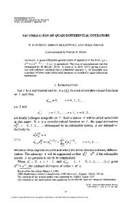
However, if one wants to express the derivatives of the built-in function Abs in terms of DiracDelta functions then one has to resort to distributions. The Mathematica function Abs[x] has to be redefined in terms of a distribution abs[x] such that : absx_: x HeavisideThetax  HeavisideThetax FramedPlotabsx,x,2,2, PlotLabel StyleStringJoin"absx  ",ToStringabsx,tF,"\n",9, LabelStyle DirectiveBold,Tiny,FontFamily "Helvetica",ImageSize 150

absx  x x  x 2.0

1.5

1.0

0.5

2

1

1

2

The first few derivatives of the distribution abs[x] turn out to be :

12th International Mathematica Symposium, 2015, Prague, Czech Republic

20 / 20

FullSimplify  Tablex,n absx,n,0,5tF x x  x, x  x, 2 x, 2  x, 2  x, 2 3 x As regards to the representation of the unit step function note the distinction that procedure UnitStep is a function whereas HeavisideTheta is a distribution . Therefore, w.r.t. x=0 one obtains for UnitStep[0]=1 , whereas the value for HeavisideTheta[0] is not defined.

? UnitStep HeavisideTheta

Acknowledgments The author would like to thank Vladimir Gerdt from JINR, Dubna/Russia for his suggestions and Leonid Shifrin, WRI consultant in St. Petersburg/Russia, for his patient support and competent solutions regarding sophisticated problems in Mathematica. Special thanks to Jason Harris, Michael Trott and Oliver Rübenkönig, all at WRI, for their valuable contributions and suggestions for notational improvements during the development of the implementation. Finally, the constructive help of David Park concerning the structure of Mathematica packages is gratefully acknowledged.

References P. K. Kythe, P. Puri & M. R. Schäferkotter, "Partial Differential Equations and Boundary Value Problems with Mathematica", 2nd Ed. , Chapman & Hall / CRC, 2002, Chapter 3.2-3.4, pp. 75-81. R. Kragler, "Method of Inverse Differential Operators for the Solution of PDEs," in Computer Algebra Systems in Teaching and Research, 6th International. Workshop, vol. Differential Equations, Dynamical Systems and Celestial Mechanics (CASTR 2011), Siedlce ( L. Gadomski et al. eds.), Siedlce : Wydawnictwo Collegium Mazovia, 2011 pp. 79-95. R. Kragler, "Method of Inverse Differential Operators applied to certain classes of non-homogeneous PDEs and ODEs", in Proceedings of "The Third International Conference : Mathematical Modelling and Differential Equations", Brest State University, Brest/Belarus ( Sept. 2012), Publishing Center BSU, Minsk, 2012 pp. 290-307, ISBN 978-985-553-054-2 Martha L Abell & James P. Braselton, “Differential Equations with Mathematica”, 2nd Ed. , Academic Press , 1997, Chapter 11.2, pp. 723-737. Selwyn Hollis, “ A Mathematica Companion for Differential Equations” 2nd Ed., Prentice Hall/Pearson Education , 2003, Chapter 11.1, pp. 227-233.

12th International Mathematica Symposium, 2015, Prague, Czech Republik