REVIEW ARTICLE published: 21 August 2014 doi: 10.3389/fnins.2014.00253
Methodological challenges and solutions in auditory functional magnetic resonance imaging Jonathan E. Peelle* Department of Otolaryngology, Washington University in St. Louis, St. Louis, MO, USA
Edited by: Pedro Antonio Valdes-Sosa, Centro de Neurociencias de Cuba, Cuba Reviewed by: Sibylle C. Herholz, Deutsches Zentrum für Neurodegenerative Erkrankungen, Germany Dezhong Yao, University of Electronic Science and Technology of China, China *Correspondence: Jonathan E. Peelle, Department of Otolaryngology, Washington University in St. Louis, 660 South Euclid, Box 8115, St. Louis, MO 63110, USA e-mail:
[email protected]
Functional magnetic resonance imaging (fMRI) studies involve substantial acoustic noise. This review covers the difficulties posed by such noise for auditory neuroscience, as well as a number of possible solutions that have emerged. Acoustic noise can affect the processing of auditory stimuli by making them inaudible or unintelligible, and can result in reduced sensitivity to auditory activation in auditory cortex. Equally importantly, acoustic noise may also lead to increased listening effort, meaning that even when auditory stimuli are perceived, neural processing may differ from when the same stimuli are presented in quiet. These and other challenges have motivated a number of approaches for collecting auditory fMRI data. Although using a continuous echoplanar imaging (EPI) sequence provides high quality imaging data, these data may also be contaminated by background acoustic noise. Traditional sparse imaging has the advantage of avoiding acoustic noise during stimulus presentation, but at a cost of reduced temporal resolution. Recently, three classes of techniques have been developed to circumvent these limitations. The first is Interleaved Silent Steady State (ISSS) imaging, a variation of sparse imaging that involves collecting multiple volumes following a silent period while maintaining steady-state longitudinal magnetization. The second involves active noise control to limit the impact of acoustic scanner noise. Finally, novel MRI sequences that reduce the amount of acoustic noise produced during fMRI make the use of continuous scanning a more practical option. Together these advances provide unprecedented opportunities for researchers to collect high-quality data of hemodynamic responses to auditory stimuli using fMRI. Keywords: auditory cortex, auditory perception, speech, music, hearing, executive function
INTRODUCTION
SOURCES OF ACOUSTIC INTERFERENCE IN fMRI
Over the past 20 years, functional magnetic resonance imaging (fMRI) has become the workhorse of cognitive scientists interested in noninvasively measuring localized human brain activity. Although the benefits provided by fMRI have been substantial, there are numerous ways in which it remains an imperfect technique. This is perhaps nowhere more true than in the field of auditory neuroscience due to the substantial acoustic noise generated by standard fMRI sequences. In order to study brain function using fMRI, auditory researchers face what can seem like an unappealing array of methodological decisions that impact the acoustic soundscape, cognitive performance, and imaging data characteristics to varying degrees. Here I review the challenges faced in auditory fMRI studies, possible solutions, and prospects for future improvement. Much of the information regarding the basic mechanics of noise in fMRI can be found in previous reviews (Amaro et al., 2002; Moelker and Pattynama, 2003; Talavage et al., 2014); although I have repeated the main points for completeness, I focus on more recent theoretical perspectives and methodological advances.
Table 1 summarizes several factors that contribute to the degradation of acoustic signals during fMRI. Echoplanar imaging (EPI) sequences commonly used to detect the blood oxygen level dependent (BOLD) signal in fMRI require radiofrequency (RF) pulses that excite tissue and gradient coils that help encode spatial position by altering the local magnetic field. During EPI the gradient coils switch between phase encoding and readout currents, producing Lorentz forces that act on the coils and connecting wires. These vibrations travel as compressional waves through the scanner hardware and eventually enter the air as acoustic sound. This gradient-induced vibration produces the most prominent acoustic noise during fMRI, and can continue for up to approximately 0.5 s after the gradient activity ceases (Ravicz et al., 2000). Because the Lorentz force is proportional to the main magnetic field strength (B0 ) and the gradient current, both high B0 and high gradient amplitudes generally increase the amount of acoustic noise generated (Moelker et al., 2003). For example, increasing field strength from 0.2 to 3 T will bring maximum acoustic noise from ∼85 to ∼130 dB SPL (Foster et al., 2000; Ravicz et al., 2000; Price et al., 2001).
www.frontiersin.org
August 2014 | Volume 8 | Article 253 | 1
Peelle
Auditory fMRI
Table 1 | Sources of acoustic interference during fMRI. Source
Approximate noise level (dB SPL)
Gradient coils Helium pump and air circulating In-ear foam earplugs Sub-optimal headphones
85–130 57–76 – –
Although the noise generated by gradient switching is the most obvious (i.e., loudest) source of acoustic noise during fMRI, it is not the only source of acoustic interference. RF pulses contribute additional acoustic noise, and noise is also present as a result of air circulation systems and helium pumps in the range of 57–76 dB SPL (Ravicz et al., 2000). Because RF and helium pump noise is substantially quieter than that generated by gradient coils it probably provides a negligible contribution when scanning is continuous, but may be more relevant in sparse or interleaved silent steady state (ISSS) imaging sequences (described in a later section) when gradient-switching noise is absent. Auditory clarity can also be reduced as a result of in-ear hearing protection and sub-optimal headphone systems. Separately or together, these noise sources provide a level of acoustic interference that is significantly higher than that found in a typical behavioral testing environment. In the next section I turn to the more interesting question of the various ways in which this cacophony may impact auditory neuroscience.
CHALLENGES OF ACOUSTIC NOISE IN AUDITORY fMRI Acoustic noise can influence neural response through at least three independent pathways, illustrated schematically in Figure 1. The effects will vary depending on the specific stimuli, population being studied, and brain networks being examined. Importantly, though, in many cases the impact of noise on brain activation can be seen outside of auditory cortex. In this section I review the most pertinent challenges caused by acoustic scanner noise. ENERGETIC MASKING
Energetic masking refers to the masking of a target sound by a noise or distractor sound that obscures information in the target. That is, interference occurs at a peripheral level of processing, with the masker already obscuring the target as the sound enters the eardrum (and thus at the most peripheral levels of the auditory system). The level of masking is often characterized by the signal-to-noise ratio (SNR), which reflects the relative loudness of the signal and masker. For example, an SNR of +5 dB indicates that on average the target signal is 5 dB louder than the masker. If scanner noise at a subject’s ear is 80 dB SPL, achieving a moderately clear SNR of +5 would require presenting a target signal at 85 dB SPL. When considering the masking effects of noise it is important to note that the characteristics of the noise are also important: noise that has temporal modulation can permit listeners to glean information from the “dips” in the noise masker. Energetic masking highlights the most obvious challenge of using auditory stimuli in fMRI: Subjects may not be able to perceive auditory stimuli due to scanner noise. If stimuli are inaudible—or less than fully perceived in some way—interpreting the subsequent neural responses can be problematic. A different
Frontiers in Neuroscience | Brain Imaging Methods
scanner noise
auditory cortex activation
stimulus degradation
participant discomfort
reduced sensitivity
executive challenge
attentional challenge
premotor cortex
frontal-parietal
inferior frontal gyrus
...
auditory pathway
cingulo-opercular network FIGURE 1 | Even when subjects can hear stimuli, acoustic noise can impact neural activity through at least three pathways. First, acoustic noise from the scanner stimulates the auditory pathway (including auditory cortex), reducing sensitivity to experimental stimuli. Second, successfully processing degraded stimuli may require additional executive processes (such as verbal working memory or performance monitoring). These executive processes are frequently found to rely on regions of frontal and premotor cortex, as well as the cingulo-opercular network. Finally, scanner noise may increase attentional demands, even for non-auditory tasks, an effect that is likely exacerbated in more sensitive subject populations. Although the specific cognitive and neural consequences of these challenges may vary, the critical point is that scanner noise can alter both cognitive demand and the patterns of brain activity observed through multiple mechanisms, affecting both auditory and non-auditory brain networks.
(but related) sort of energetic masking challenge arises in experiments in which subjects are required to make vocal responses, as scanner noise can interfere with an experimenter’s understanding of subject responses; in some cases this can be ameliorated by offline noise reduction approaches (e.g., Cusack et al., 2005). In addition, the presence of acoustic noise may also change the quality of vocalizations produced by subjects (Junqua, 1996). Acoustic noise thus impacts not only auditory perception, but speech production, which may be important for some experimental paradigms. Two ways of ascertaining the degree to which energetic masking is a problem are (1) to ask participants about their subjective experience hearing stimuli or (2) to include a discrimination or recall test that can empirically verify the degree to which auditory stimuli are perceived. Given individual differences in hearing level and ability to comprehend stimuli in noise, these are likely best done for each subject, rather than, for example, audibility being verified solely by the experimenter. It is also important to test audibility using stimuli representative of those used in the experiment, as the masking effects of scanner noise can be influenced by specific acoustic characteristics of the target stimuli (for example, being more detrimental to perception of birdsong than speech).
August 2014 | Volume 8 | Article 253 | 2
Peelle
Although it is naturally important for subjects to be able to hear experimental stimuli (and for experimenters to hear subject responses, if necessary), the requirement of audibility is obvious enough that it is often taken into account when designing a study. However, acoustic noise may also cause more pernicious challenges, to which I turn in the following sections. AUDITORY ACTIVATION
A natural concern regarding acoustic noise during fMRI relates to the activation along the auditory pathway resulting from the scanner noise. If brain activity is modulated in response to scanner noise, might this reduce our ability to detect signals of interest? To investigate the effect of scanner noise on auditory activation, Bandettini et al. (1998) acquired data with and without EPI-based acoustic stimulation, enabling them to compare brain activity that could be attributed to scanner noise. They found that scanner noise results in increased activity bilaterally in superior temporal cortex (see also Talavage et al., 1999). Notably, this activity was not observed only in primary auditory cortex, but in secondary auditory regions as well. The timecourse of activation to scanner noise peaks 4–5 s after stimulus onset, returning to baseline by 9–12 s (Hall et al., 2000), and is thus comparable to that observed in other regions of cortex (Aguirre et al., 1998). Scanner-related activation in primary and secondary auditory cortex limits the dynamic range of these regions, producing weaker responses to auditory stimuli (Shah et al., 1999; Talavage and Edmister, 2004; Langers et al., 2005; Gaab et al., 2007). In addition to overall changes in magnitude or spatial extent of auditory activation, scanner noise can affect the level at which stimuli need to be presented for audibility, which can in turn affect activity down to the level of tonotopic organization (Langers and van Dijk, 2012). Thus, if activity along the auditory pathway proper is of interest, the contribution of scanner noise must be carefully considered when interpreting results. It is worth noting that while previous studies have investigated the effect of scanner noise on overall (univariate) response magnitude, the degree to which this overall change in gain may affect multivariate analyses is unclear. Again, this is true for activity in both auditory cortex and regions further along the auditory processing hierarchy (Davis and Johnsrude, 2007; Peelle et al., 2010b).
Auditory fMRI
evidence supporting the link between acoustic challenge and cognitive resources comes from pupillometry (Kuchinsky et al., 2013; Zekveld and Kramer, 2014) and visual tasks which relate to individual differences in speech perception ability (Zekveld et al., 2007; Besser et al., 2012). The additional cognitive resources required are not specific to acoustic processing but appear to reflect more domain-general processes (such as verbal working memory) recruited to help with auditory processing (Wingfield et al., 2005; Rönnberg et al., 2013). Thus, acoustic challenge can indirectly impact a wide range of cognitive operations. Consistent with this shared resource view, behavioral effects of acoustic clarity are reliably found on a variety of tasks. Van Engen et al. (2012) compared listeners’ recognition memory for sentences spoken in conversational speech compared to those spoken in a clear speaking style (with accentuated acoustic features), and found that memory was superior for the acoustically-clearer sentences. Likewise, listeners facing acoustic challenge—due to background noise, degraded speech, or hearing impairment— perform poorer than listeners with normal hearing on auditory tasks ranging from sentence processing to episodic memory tasks (Pichora-Fuller et al., 1995; Surprenant, 1999; Murphy et al., 2000; McCoy et al., 2005; Tun et al., 2010; Heinrich and Schneider, 2011; Lash et al., 2013). Converging evidence for the neural effects of effortful listening comes from fMRI studies in which increased neural activity is seen for degraded speech relative to unprocessed speech (Scott and McGettigan, 2013), illustrated in Figure 2. Davis and
Clear speech
Degraded speech
core speech network
core speech network + executive support
COGNITIVE EFFORT DURING AUDITORY PROCESSING
Although acoustic noise can potentially affect all auditory processing, most of the research on the cognitive effects of acoustic challenge has occurred in the context of speech comprehension. There is increasing consensus that decreased acoustic clarity requires listeners to engage additional cognitive processing to successfully understand spoken language. For example, after hearing a list of spoken words, memory is worse for words presented in noise, even though the words themselves are intelligible (Rabbitt, 1968). When some words are presented in noise (but are still intelligible), subjects have difficulty remembering not only the words in noise, but prior words (Rabbitt, 1968; Cousins et al., 2014), suggesting an increase in cognitive processing for degraded speech that lasts longer than the degraded stimulus itself and interferes with memory (Miller and Wingfield, 2010). Additional
www.frontiersin.org
FIGURE 2 | Listening to degraded speech requires increased reliance on executive processing and a more extensive network of brain regions. When speech clarity is high, neural activity is largely confined to traditional frontotemporal “language” regions including bilateral temporal cortex and left inferior frontal gyrus. When speech clarity is reduced, additional activity is frequently seen in frontal cortex, including middle frontal gyrus, premotor cortex, and the cingulo-opercular network (consisting of bilateral frontal operculum and anterior insula, as well as dorsal anterior cingulate) (Dosenbach et al., 2008).
August 2014 | Volume 8 | Article 253 | 3
Peelle
Johnsrude (2003) presented listeners with sentences that varied in their intelligibility, with speech clarity ranging from unintelligible to fully intelligible. They found greater activity for degraded speech compared to fully intelligible speech in the left hemisphere, along both left superior temporal gyrus and inferior frontal cortex. Importantly, increased activity in frontal and prefrontal cortex was greater for moderately distorted speech than either fully intelligible or fully unintelligible speech (i.e., an inverted U-shaped function), consistent with its involvement in recovering meaning from degraded speech (as distinct from a simple acoustic response). Acoustic clarity (i.e., SNR) also impacts the brain networks supporting semantic processing during sentence comprehension (Davis et al., 2011), possibly reflecting increased use of semantic context as top-down knowledge during degraded speech processing (Obleser et al., 2007; Obleser and Kotz, 2010; Sohoglu et al., 2012). Additional studies using various forms of degraded speech have also found difficulty-related increases in regions often associated with cognitive control or performance monitoring, such as bilateral insula and anterior cingulate cortex (Eckert et al., 2009; Adank, 2012; Wild et al., 2012; Erb et al., 2013; Vaden et al., 2013). The stimuli used in these studies are typically less intelligible than unprocessed speech (e.g., 4- or 6-channel vocoded1 speech, or low-pass filtered speech). Thus, although the increased recruitment of cognitive and neural resources to handle degraded speech is frequently observed, the specific cognitive processes engaged— and thus the pattern of neural activity—depend on the degree of acoustic challenge presented. An implication of this variability is that it may be hard to predict a priori the effect of acoustic challenge on the particular cognitive system(s) of interest. In summary, there is clear evidence that listening to degraded speech results in increased cognitive demand and altered patterns of brain activity. The specific differences in neural activity depend on the degree of the acoustic challenge, and thus may differ between moderate levels of degradation (when comprehension accuracy remains high and few errors are made) and more severe levels of degradation (when comprehension is significantly decreased). It is important to note that effort-related differences in brain activity can be seen both within the classic speech comprehension network and in regions less typically associated with speech comprehension, and depend on the nature of both the stimuli and the task. Furthermore, the way in which these effort-related increases interact with other task manipulations has received little empirical attention, and thus the degree to which background noise may influence observed patterns of neural response for many specific tasks is largely unknown. Finally, although most of the research on listening effort has been focused on speech comprehension, it is reasonable to think that many of these same principles might transfer to other auditory domains, such as music or environmental sounds. And, 1 Noise vocoding (Shannon et al., 1995) involves dividing the frequency spectrum of a stimulus into bands, or channels. Within each channel, the amplitude envelope is extracted and used to modulate broadband noise. Thus, the number of channels determines the spectral detail present in a speech signal, with more channels resulting in a more detailed (and for speech, more intelligible) signal (see Figure 2 in Peelle and Davis, 2012).
Frontiers in Neuroscience | Brain Imaging Methods
Auditory fMRI
as covered in the next section, effects of acoustic challenge need not even be limited to auditory tasks. EFFECTS OF ACOUSTIC NOISE IN NON-AUDITORY TASKS
Although the interference caused by acoustic noise is most obvious when considering auditory tasks, it may also affect subjects’ performance on non-auditory tasks (for example, by increasing demands on attention systems). The degree to which noise impacts non-auditory tasks is an important one for cognitive neuroscience. Unfortunately, there have been relatively few studies addressing this topic directly. Using continuous EPI, Cho et al. (1998a) had subjects perform simple tasks in the visual (flickering checkerboard) and motor (finger tapping) domains, with and without additional scanner noise played through headphones. The authors found opposite effects in visual and motor modalities: activity in visual cortex was increased with added acoustic noise, whereas activity in motor cortex was reduced. To investigate the effect of scanner noise on verbal working memory, Tomasi et al. (2005) had participants to perform an n-back task using visually-displayed letters. The loudness of the EPI scanning was varied by approximately 12 dB by selecting two readout bandwidths to minimize (or maximize) the acoustic noise. No difference in behavioral accuracy was observed as a function of noise level. However, although the overall spatial patterns of task-related activity were similar, brain activity differed as a function of noise. The louder sequence was associated with increased activity in several regions including large portions of (primarily dorsal) frontal cortex and cerebellum, and the quieter sequence was associated with greater activity in (primarily ventral) regions of frontal cortex and left temporal cortex. Behaviorally, recorded scanner noise has been shown to impact cognitive control (Hommel et al., 2012); additional effects of scanner noise have been reported in fMRI tasks of emotional processing (Skouras et al., 2013) and visual mental imagery (Mazard et al., 2002). Thus, MRI acoustic noise influences brain function across a number of cognitive domains. It is not only the loudness of scanner noise that is an issue, but also the characteristics of the sound: whether an acoustic stimulus is pulsed or continuous, for example, can significantly impact both auditory and attentional processes. Haller et al. (2005) had participants perform a visual n-back task, using either a conventional EPI sequence or one with a continuous sound (i.e., not pulsed). Although behavioral performance did not differ across sequence, there were numerous differences in the detected neural response. These included greater activity in cingulate and portions of frontal cortex for the conventional EPI sequence, but greater activity in other portions of frontal cortex and left middle temporal gyrus for the continuous noise sequence. As with conventional EPI sequences, scanner noise is once again found to impact neural processing in areas beyond auditory cortex (see also Haller et al., 2009). It is worth noting that not every study investigating this issue has observed effects of acoustic noise in non-auditory tasks: Elliott et al. (1999), using participants performing visual, motor, and auditory tasks, found that scanner noise resulted in decreased activity uniquely during the auditory condition. Nevertheless, the
August 2014 | Volume 8 | Article 253 | 4
Peelle
Auditory fMRI
number of instances in which scanner noise has been found to affect neural activity on non-auditory tasks is high enough that the issue should be taken seriously: Although exactly how much of the difference in neural response can be attributed to scanner noise is debatable, converging evidence indicates that the effects of scanner noise frequently extend beyond auditory cortex (and auditory tasks). These studies suggest that (1) a lack of behavioral effect of scanner noise does not guarantee equivalent neural processing; (2) both increases and decreases in neural activity are seen in response to scanner noise; and (3) the specific regions in which noise-related effects are observed vary across study. OVERALL SUBJECT COMFORT AND SPECIAL POPULATIONS
An additional concern regarding scanner noise is that it may increase participant discomfort. Indeed, acoustic noise can cause anxiety in human subjects (Quirk et al., 1989; Meléndez and McCrank, 1993), a finding which may also extend to animals. Scanner noise presents more of a challenge for some subjects than others, and it may be possible to improve the comfort of research subjects (and hopefully their performance) by reducing the amount of noise during MRI scanning. Additionally, if populations of subjects differ in a cognitive ability such as auditory attention, the presence of scanner noise may affect one group more than another. For example, age can significantly impact the degree to which subjects are bothered by environmental noise (Van Gerven et al., 2009); similarly, individual differences in noise sensitivity may contribute to (or reflect) variability in the effects of scanner noise on neural response (Pripfl et al., 2006). These concerns may be particularly relevant in clinical or developmental studies with children, participants with anxiety or other psychiatric condition, or participants who are particularly bothered by auditory stimulation. A CAUTIONARY NOTE REGARDING INTERACTIONS
One argument sometimes made in auditory fMRI studies using standard EPI sequences is that although acoustic noise may have some overall impact, because noise is present during all experimental conditions it cannot influence the results when comparing across conditions (which is often of most scientific interest). Given the ample amount of evidence for auditory-cognitive interactions, such an assumption seems tenuous at best. If anything,
there is good reason to suspect interactions between acoustic noise and task difficulty, which may manifest differently depending on particular stimuli, listeners, and statistical methods (for example, univariate vs. multivariate analyses). In the absence of empirical support to the contrary, claims that acoustic noise is unimportant should be treated with skepticism.
SOLUTIONS FOR AUDITORY fMRI Although at this point the prospects for auditory neuroscience inside an MRI scanner may look bleak, there is still cause for optimism. In this section I provide an overview of several methods for dealing with scanner noise that have been employed, noting advantages and disadvantages of each. These approaches are listed in Table 2, a subset of which is shown in Figure 3. PASSIVE HEARING PROTECTION
Subjects in MRI studies typically wear over-ear hearing protection that attenuates acoustic noise by approximately 30 dB. Subjects may also wear insert earphones, or foam earplugs that can provide additional reduction in acoustic noise of 25–28 dB, for a combined reduction of approximately 40 dB (Ravicz and Melcher, 2001). Although hearing protection can reduce the acoustic noise perceived during MRI, it cannot eliminate it completely: Even if perfect acoustic isolation could be achieved at the outer ear, sound waves still travel to the cochlea through bone conduction. Thus, hearing protection is only partial solution, and some degree of auditory stimulation during conventional fMRI is unavoidable. In addition, passive hearing protection may change the frequency spectrum of stimuli, affecting intelligibility or clarity. CONTINUOUS SCANNING USING A STANDARD EPI SEQUENCE
One approach in auditory fMRI is to present stimuli using a conventional continuous scanning paradigm, taking care to ensure that participants are able to adequately hear the stimuli (Figure 4A). This approach generally assumes that, because scanning noise is consistent across experimental condition, it is unlikely to systematically affect comparisons among conditions (typically what is of interest). I have already noted above the danger of this assumption with respect to additional task effects and ubiquitous interactions between perceptual and cognitive factors. However, for some paradigms a continuous scanning paradigm
Table 2 | Methods for dealing with acoustic noise in fMRI. Approach
Approximate noise Requires custom Requires custom Requires custom Image quality reduction during scanner presentation MRI sequence? relative to stimulus (dB)a hardware? equipment? continuous
Temporal resolution relative to continuous
Continuous EPI
0
No
No
No
–
–
Passive hearing protection
35
No
No
No
No change
No change
Sparse imaging
50
No
No
No
No change
Reduced
ISSS imaging
50
No
No
Yes
No change
Slightly reduced
Active noise control
40
No
Yes
No
No change
No change
Quiet MRI sequences
20
No
No
Yes
Reduced
Slightly reduced
Scanner hardware modification
20
Yes
No
No
No change
No change
a The
actual reduction of acoustic noise can vary substantially depending on the specific equipment and implementation; these numbers are provided as a rough
estimate.
www.frontiersin.org
August 2014 | Volume 8 | Article 253 | 5
Peelle
Auditory fMRI
~1 s
temporal resolution
active noise control
quiet EPI sequences
standard EPI
ISSS imaging
sparse imaging
~20 s 60
80
100
acoustic noise during stimuli (dBA) FIGURE 3 | Schematic illustration of the relationship between temporal resolution and acoustic noise during stimulus presentation for various MRI acquisition approaches. Although the details for any specific acquisition depend on a combination of many factors, in general significant reductions in acoustic noise are associated with poorer temporal resolution.
may be acceptable. From an imaging perspective continuous imaging will generally provide the largest quantity of data, and no special considerations are necessary when analyzing the data. Continuous EPI scanning has been used in countless studies to identify brain networks responding to environmental sounds, speech, and music. The critical question is whether the cognitive processes being imaged are actually the ones in which the experimenter is interested2. SPARSE IMAGING
When researchers are concerned about acoustic noise in fMRI, by far the most widely used approach is sparse imaging, also referred to as clustered volume acquisition (Scheffler et al., 1998; Eden et al., 1999; Edmister et al., 1999; Hall et al., 1999; Talavage and Hall, 2012). In sparse imaging, illustrated in Figure 4B, the repetition time (TR) is set to be longer than the acquisition time (TA) of a single volume. Slice acquisition is clustered toward the end of a TR, leaving a period in which no data are collected. This intervening period is relatively quiet due to the lack of gradient switching, and permits stimuli to be presented in more favorable acoustic conditions. Because of the inherent lag of the hemodynamic response (typically 4–7 s to peak), the scan following stimulus presentation can still measure responses to stimuli, including the peak response if presentation is timed appropriately. 2 For
researchers who question whether acoustic noise during fMRI may impact cognitive processing, it may be interesting to suggest to a cognitive psychologist that they play 100 dB SPL sounds during their next behavioral study and gauge their enthusiasm.
Frontiers in Neuroscience | Brain Imaging Methods
The primary disadvantage of sparse imaging is that due to the longer TR, less information is available about the timecourse of the response (i.e., there is a lower sampling rate). In addition to reducing the accuracy of the response estimate, the reduced sampling rate also means that differences in timing of response may be interpreted as differences in magnitude. An example of this is shown in Figure 4B, in which hemodynamic responses that differ in magnitude and timing will give different results, depending on the time at which the response is sampled. The lack of timecourse information in sparse imaging can be ameliorated in part by systematically varying the delay between the stimulus and volume collection (Robson et al., 1998; Belin et al., 1999), illustrated in Figure 4D. In this way, the hemodynamic response can be sampled at multiple time points relative to stimulus onset over different trials. Thus, across trials, an accurate temporal profile for each category of stimulus can be estimated. Like all event-related fMRI analyses this approach assumes a consistent response for all stimuli in a given category. It also may require prohibitively long periods of scanning to sample each stimulus at multiple points; this requirement has meant that in practice varying presentation times relative to data collection is done infrequently. Many studies incorporating sparse imaging use an eventrelated design, along with TRs in the neighborhood of 16 s or greater, in order to allow scanner-induced BOLD response to return to near baseline levels on each trial. Although this may be particularly helpful for experiments in which activity in primary auditory areas is of interest, it is not necessary for all studies, and in principle sparse designs can use significantly shorter TRs (e.g.,