THEORETICAL & EXPERIMENTAL STUDIES
AIHA Journal
64:604–608 (2003)
AUTHORS F. Marzala E. Gonza´lezb A. Min ˜ anab A. Baezab Universidad Polite´cnica de Cartagena, Departamento de Ingenierı´a Te´rmica y de Fluidos, Paseo de Alfonso XIII, 48, 30203 Cartagena, Murcia, Spain; e-mail:
[email protected]; b Universidad de Murcia, Departamento de Ingenierı´a Quı´mica, 30071 Espinardo, Murcia, Spain a
Ms. #400
Methodologies for Determining Capture Efficiencies in Surface Treatment Tanks Methodologies are proposed for determining capture efficiencies in the ventilation systems of surface treatment tanks, using test-scale equipment. The equipment, which incorporates a lateral and push-pull ventilation system, can measure and control the variables of interest because it incorporates a tracer gas generator (sulfur hexafluoride, the concentration of which is measured by infrared spectrometer). The experimental methodologies described determine total efficiency (when the tracer is emitted uniformly from the whole surface of the tank) and the so-called transversal linear efficiency (when the tracer is emitted linearly through a perforated tube situated over the tank, parallel to the exhaust hood face). The analytical and graphical relationships that can be are established between the two efficiencies make it possible to detect where the emissions not captured by the ventilation system are produced (i.e., losses to the outside). At the same time, such losses can be quantified. Several experiments, results of which are analyzed by the methods described, are included. Keywords: capture efficiency, open surface tank ventilation, push-pull ventilation, tracer gas, transversal linear efficiency
T
he emission of contaminants from surface treatment tanks is controlled by lateral exhaust or push-pull systems.(1,2) The former generate omnidirectional velocity fields around the tank, which means that the capture efficiency decreases rapidly as the distance from the exhaust hood increases.(3) In push-pull systems the pushed air forms a curtain parallel to the tank surface (wall jet), which drags the emissions toward the exhaust.(4–9) This means that higher capture efficiencies are possible than with lateral exhaust systems, because random currents in the environment do not distort the push flows to the same extent.(10–12) Capture efficiency is determined by the ratio of the amount of pollutant captured by the system to the amount generated at the source. The measurement of pollutants from industrial tanks presents numerous difficulties due to the heterogeneity of the components and the variable dynamics of the emission itself, which are typical of nonstationary processes. It is even more difficult to determine the flow emitted to the workplace because of the dispersion and dilution provoked by air currents and external convection, not to 604
AIHA Journal (64)
September/October 2003
mention the emissions produced by nearby processes. For these reasons it is convenient to use test installations and tracer gases, the behavior of which closely reflects that of real systems.(13,14) This article describes methodologies for determining the capture efficiency of a push-pull system and how they were checked in a specially designed test installation.(15)
MATERIALS AND METHODS Test Installation An overall diagram of the installation is shown in Figure 1. The experimental equipment consisted of three interconnected zones: the push unit, the tank, and the exhaust unit. In the first zone an air current was generated that carried the tracers emitted by the tank toward the exhaust hood, through which they were exhausted to the outside. The study was carried out in an enclosed area with air velocities of less than 0.1 m/sec. The surface tank, measuring 1.80 in length and 1.6 m in width, was perforated with 460 holes connected to a gas grid for distributing the
Copyright 2003, American Industrial Hygiene Association
THEORETICAL & EXPERIMENTAL STUDIES
FIGURE 1. Overview of the test installation. 1: Tank; 1a: diffuser tube; 2: exhaust system; 2a: hood; 2b: venturi; 2c: fan; 2d: chimney; 3: push system; 3a: plenum; 3b: venturi; 4: control systems; 4a: infrared spectrometer; 4b: frequency converter fan; 4c: flow meter pull; 4d: tank temperature control; 4e: flow meter push; 5: tracer gas systems: F6S generator
tracer gas (sulfur hexafluoride). Each orifice was fitted with a 0.3mm diameter needle to ensure the uniform emission of tracer. A system of electrical resistances allowed the homogeneous heating of the surface to 1008C. The exhaust hood had a rectangular entrance 30 cm high and 1.60 cm wide. The uniformity of the velocity at the exhaust hood
Nomenclature Ca: CaT: Cax: D: ET: Ex,x1Dx: gax: gpx: gx: Gax,ax1Dx: Gpx,px1Dx: GT: GTx,Tx1Dx: H: l: L: Dl: n: N: Qa: Qi: Tamb: Ttank: W: x:
Concentration of F6S captured by the exhaust system from the tracer gas injected through the n rows of holes, mg/m3. Concentration of F6S injected directly into the exhaust system, mg/m3. Concentration of F6S captured by the exhaust system from the diffuser tube in position x, mg/m3. Diameter holes in the push tube, mm. Capture efficiency, dimensionless. Transversal linear capture efficiency in position x or x1Dx, dimensionless. Mass flow of F6S captured by the exhaust system from the x row, mg/sec. Mass flow of F6S lost to the exterior from the x row, mg/sec. Mass flow of F6S injected through the x row, mg/sec. Mass flow of tracer captured by the exhaust system from the diffuser tube in positions x or x1Dx, mg/sec. Mass flow of tracer lost to the exterior from the diffuser tube in positions position x or x1Dx, mg/sec. Total mass flow of tracer, mg/sec. Mass flow of tracer injected through the diffuser tube situated over the tank in positions x or x1Dx, mg/sec. Hood width, m. Length measured on tank surface from push unit, m. Tank length, m. Distance between two consecutive rows of holes, m. Rows of holes parallel to the exhaust hood face. Number of holes in the push tube. Pull flow, m3/sec. Initial push flow, m3/sec. Ambient temperature, 8C Tank temperature, 8C Hood length or tank width, m. Distance from push to a row of holes or diffuser tube, m.
FIGURE 2. A: Perforated tube used in push unit; B: assembly containing the perforated tube
inlet was checked for the lateral flows ventilation system. The exhaust flow can be regulated between 0.08 and 2.5 m3/sec by adjusting the fan rotation rate. The push unit (Figure 2) was made up of tubing (1.6 m in length and 50 mm in diameter). The tube was closed at both ends and perforated by holes of 10 mm diameter. The posterior part of the tube contained a 20-mm wide slot running the whole length to facilitate the uniform velocity distribution of the air jets. The tube was situated at one end of the plenum. Its circular shape made it possible to vary the angle of the jets from 08 (parallel to the tank surface) to 458. The flow could be regulated from 0.0025 to 0.4 m3/sec by varying the fan rotation rate. The flow of sulfur hexafluoride was kept constant (from 55 to 75 cm3/min) and was mixed with air (20 L/min) to ensure rapid stabilization of its distribution in the network grid. The tracer air mixture could be injected directly inside the exhaust hood, in the network grid, or in the diffuser tube to be described later. In this last case the mass flow of the tracer was kept constant, but the dilution airflow was decreased. The tracer gas diffuser tube (Figure 1, 1a) consisted of a 10mm diameter tube closed at both ends and perforated along its length with 100 holes of 0.3 mm diameter. The center was connected to the tracer gas generator. The tube could be placed in any position on the surface of the tank but was always parallel to the exhaust hood face. AIHA Journal (64)
September/October 2003
605
The same total tracer flows were used in the experiments designed to quantify total and transversal linear efficiencies. The mass flow injected in each row of holes shown in Figure 3 are all equal, so that
O g 5 ng ,
(4)
GT , n
(5)
THEORETICAL & EXPERIMENTAL STUDIES
x5n
GT 5 GTx 5
x
x
x51
where gx 5 FIGURE 3. Injection of tracer gas to determine total efficiency of the system and position of tracer gas diffuser tube for the determination of transversal linear efficiency in any position x
Given that the conditions of the experiments for determining ET and Ex are identical (equal pull and push flows, same tank length and temperature), it is verified, by analogy with both experiments for each position x (see Figure 3), that:
Tracer concentration is measured by an infrared spectrometer placed just after the venturi in the exhaust unit (Figure 1, 4a) to ensure uniform tracer air mixture.
gax G 5 ax gx GT or
Methodologies for Determining Efficiencies
gax 5 gx
To determine total efficiency, the tracer gas flow, GT, was injected into the exhaust hood or into the gas grid beneath the tank, where it was emitted uniformly through the surface (see Figure 3). In the first case the tracer gas was injected directly into the hood, where it mixed with the exhaust flow, Qa. The concentration of the mixture, CaT, which represents the maximum reference value, was thus determined. In the second case Sx5n x51 gx was injected from the tank surface through the n rows of holes parallel to the exhaust hood face. Part of this tracer gas, Sx5n x51 gpx, was lost to the exterior and the rest was captured by the exhaust system, Sx5n x51 gax, giving the concentration Ca. So, taking into consideration Figure 3 and previous comments:
Og 5Og 1Og
x5n
GT 5
x5n
x
x5n
ax
x51
x51
px
(1)
x51
The total capture efficiency of the system, ET, was defined as the ratio between the captured tracer flow and that injected directly into the exhaust hood, which was calculated from the quotient of the concentrations:
Og
x5n
ET 5
x51
GT
ax
5
Q aCa Ca 5 Q aCaT CaT
Ex 5
Gax QC C 5 a ax 5 ax GT Q aCaT CaT
(3)
that is, it is determined as the quotient of concentrations obtained when tracer was injected through the diffuser in x and the reference. The analytical and graphical relation between total and transversal linear efficiencies makes it possible to interpret the behavior of the system. 606
AIHA Journal (64)
September/October 2003
Gax GT
(7)
Substituting Equations 7 and 5 in Equation 2 and bearing in mind Equation 3:
O Gn
x5n
ET 5
x51
GT
O
x5n
ax
5
G 1 x51 ax 1 5 n GT n
OE
x5n
x
(8)
x51
On the other hand, according to Figure 3, and bearing in mind that the first and last row of holes are separated from the end of the tank by the same distance that separates consecutive rows (Dl), we obtain: n 5 (L/Dl) 2 1
(9)
where Dl is the distance separating two consecutive rows. Substituting Equations 9 in Equation 8 gives:
O L 2Dl Dl E
x5n
ET 5
x
(10)
x51
Taking limits for n → ` and consequently, Dl → dx (equivalent to a continuous and uniform injection over the whole surface of the tank):
(2)
To determine the transversal linear efficiency, the tracer gas was injected sequentially into the exhaust hood or through the diffuser tube situated over the tank (Figure 1, 1a; and Figure 3). The concentrations CaT (reference) and Cax (obtained from Gax) were measured as in the previous case, and then the diffuser tube was moved to other positions. The transversal linear capture efficiency in any position x, Ex (Figure 3) is defined as:
(6)
ET 5
1 L
E
L
Ex dx
(11)
0
This expression makes it possible to relate ET and Ex as long as the geometric and operative variables are identical in both experiments.(16) Regarding the graphical relationship between the types of efficiency, a typical push-pull profile obtained when Ex is represented as a ratio to tank length (Figure 4B) is described. Figure 4A represents the tank and the zones where the mass balances used later were carried out. In the case of Figure 4B, Equation 11 establishes that total efficiency can be determined by the quotient: ET 5
Captured mass flow Surface area 0abcL0 5 Injected mass flow Surface area 01cL0
(12)
Thus, the mass flow not collected by the exhaust system with respect to the total injected is determined by:
THEORETICAL & EXPERIMENTAL STUDIES
FIGURE 4. A: Tank set up to determine transversal linear efficiency, showing two positions of diffuser tube, at x and x1Dx; B: typical profile of transversal linear efficiency versus tank length in push-pull
1 2 ET 5
FIGURE 5. Total capture efficiency in a tank of 1.80 m length and 1.60 m width at 508C (Ttank). Push tube: diameter of holes, 10 mm; number of holes, 52. Pull flow: 0.200 m3/sec. Tamb: 188C
Surface area a1ba Surface area 01cL0
(13)
Profile Ex of Figure 4B delimits three regions: (1) zone between l2 and L, in which the flow injected is completely captured, because Ex51 throughout the zone; (2) zone between l1 and l2, where all the losses to the exterior occur and which is characterized by variations in transversal linear efficiency. Taking into account GT and carrying out mass balance for zones MNPQM and RSPQR (Figure 4A), gives,
The third zone lies between the beginning of the push and l1, in which, as can be deduced from the previous discussion, no losses occur because the transversal linear efficiency is constant. The efficiency profile is less than unity because of the previously described losses in zone (2).
RESULTS AND DISCUSSION
In MNPQM: GTx 5 Gax 1 Gpx
(14)
GTx1Dx 5 Gax1Dx 1 Gpx1Dx
(15)
In RSPQR:
Given that (Figures 3 and 4A): GTx 5 GTx1Dx 5 GT
(16)
The following is verified: In MNPQM: 15
Gax Gpx 1 or, GT GT
1 5 Ex 1
Gpx GT
(17)
In RSPQR: 15
Gax1Dx Gpx1Dx 1 or, GT GT
1 5 Ex1Dx 1
Gpx1Dx GT
(18)
The balance in zone MNSRM is obtained by difference between Equations 17 and 18: Ex1Dx 2 Ex 5
Gpx 2 Gpx1Dx GT
(19)
f the numerous experiments carried out to check the proposed method, two are described here. Figure 5 represents the total efficiency obtained for the conditions indicated. Note the quasiparabolic shape with a maximum or plateau corresponding to values of Qi between 0.010 and 0.018 m3/sec. Of the different experiments depicted in Figure 5, those corresponding to points a and b were further analyzed by determining the transversal linear efficiency (Figures 6A and 6B, respectively). The profile of Ex in Figure 6A demonstrates that losses in efficiency are produced only in the zone of the tank surface between 400 and 600 mm from the push, because this is where the efficiency is seen to vary. This zone coincides with the place where the push jets impact over the tank.(16) On the other hand, the area over the profile is proportional to the losses, the quotient of which with the total area allows determination of the capture efficiency that corresponds to 97.1%, which agrees with the information provided by Figure 5. The profile obtained in Figure 6B shows two loss zones, the first approximately coinciding with that described in the previous case and the second produced in the exhaust hood. Just as before, the total losses of the system are proportional to the area situated above the efficiency profile.
O
so that at the limit, when Dx→0, it becomes: dEx 5
2dGpx , GT
or,
dGpx 5 2GT dEx
CONCLUSIONS
(20)
where dGpx represents the losses in the differential element. That is, the losses occur in zones where there are variations in the efficiencies Ex.
he methodologies proposed permit the total efficiency to be determined, reflecting the general behavior of the ventilation system and the so-called transversal linear efficiency, which detects the zone where losses occur in push-pull ventilation systems.
T
AIHA Journal (64)
September/October 2003
607
THEORETICAL & EXPERIMENTAL STUDIES
The relation between the two types of efficiency, which is established both analytically and graphically, helps in the understanding and application of the said methods. The results of the application of the methodologies can serve to improve the design of this type of ventilation system, and the bases of the procedures can be used to study other ventilation systems.
REFERENCES
FIGURE 6. Transversal linear efficiencies of Figure 5. A: for experiment a (Qi 5 0.020 m3/sec); B: for experiment b (Qi 5 0.030 m3/sec)
608
AIHA Journal (64)
September/October 2003
1. Institut National de Recherche et de Se´curite´ (INRS): Guide Practique de Ventilation: 2. Ventilation des Cuves et Bains de Traitmen de Surface (ED 651.30). Paris: INRS, 1989. 2. Marzal, F.J., E. Gonza´lez, A. Min ˜ ana, and A. Baeza: Analytical model for evaluating lateral capture efficiencies in surface treatment tanks. Am. Ind. Hyg. Assoc. J. 63:572–577 (2002). 3. American Conference of Governmental Industrial Hygienists (ACGIH): Industrial Ventilation: A Manual of Recommended Practice, 24th ed. Cincinnati, Ohio: ACGIH, 2001. 4. Padmanadham, G., and B.H. Lakshmana: Mean and turbulence characteristics of a class of three dimensional wall jets. Part 1: Mean flow characteristics. Trans. ASME, J. Fluids Engr. 113:620–628 (1991). 5. Katz, Y., E. Horev, and I. Wygnanski: The forced turbulent wall jet. J. Fluid. Mech. 242:577–609 (1992). 6. Robinson, M., and D.B. Ingham: Recommendations for the design of push-pull ventilation systems for open surface tanks. Ann. Occup. Hyg. 40:693–704 (1996). 7. Heiselberg, P., and C. Topp: Removal of airborne contaminants from a surface tank by a push-pull system. In Ventilation ’97 Proceedings of the 5th International Symposium on Ventilation for Contaminant Control, pp. 770–780. Ottawa, Canada, 1997. 8. Marzal, F.J., E. Gonza´lez, A. Min ˜ ana, and A. Baeza: Influence of push element geometry on the capture efficiency of push-pull ventilation systems in surface treatments tanks. Ann. Occup. Hyg. 46:383– 393 (2002). 9. Rota, R., G. Nano, and L. Canossa: Design guidelines for push-pull ventilation systems through computational fluid dynamics modeling. Am. Ind. Hyg. Assoc. J. 62:141–148 (2001). 10. Hughes, R.T.: An overview of push-pull ventilation characteristics. Appl. Occup. Environ. Hyg. 5:156–161 (1990). 11. Klein, M.K.: A demostration of NIOSH push-pull ventilation criteria. Am. Ind. Hyg. Assoc. J. 48:238–246 (1987). 12. Flynn, M.R., K. Ahn, and C.T. Miller: Three dimensional finite element simulation of a turbulent push-pull ventilation system. Ann. Occup. Hyg. 5:573–589 (1995). 13. Woods, J.N., and J.S. McKarns: Evaluation of capture efficiencies of large push-pull ventilation systems with both visual and tracer techniques. Am. Ind. Hyg. Assoc. J. 56:1208–1214 (1995). 14. Marzal, F., E. Gonza´lez, A. Min ˜ ana, and A. Baeza: Control of emissions in rectangular tanks by push-pull ventilation system: relationship of involved flows. Montajes e Instalaciones 2:89–92 (2001). 15. Marzal, F., E. Gonza´lez, A. Min ˜ ana, and A. Baeza: Open surface tanks ventilation: Some design criteria. In Ventilation 2000 Proceedings of the 6th International Symposium on Ventilation for Contaminant Control, vol. 2. Helsinki, 2000. pp. 41–44. 16. Marzal, F., E. Gonza´lez, A. Min ˜ ana, and A. Baeza: Determination and interpretation of total and transversal linear efficiencies in pushpull ventilation systems for open surface tanks. Ann. Occup. Hyg. 46: 629–635 (2002).