Margaret Burnett, Andrei Sheretov, and Gregg Rothermel. Department of Computer Science. Oregon State University, Corvallis, Oregon 97331. {burnett, andrei ...
Scaling Up a “What You See Is What You Test” Methodology to Spreadsheet Grids Margaret Burnett, Andrei Sheretov, and Gregg Rothermel Department of Computer Science Oregon State University, Corvallis, Oregon 97331 {burnett, andrei, grother}@cs.orst.edu Abstract Although there has been considerable research into ways to design visual programming environments to improve the processes of creating new programs and of understanding existing ones, little attention has been given to helping users of these environments test their programs. This feature would be particularly important for systems aimed at end users, since testing is the primary device they use to determine whether their programs are correct. To help address this need, we introduce two visual approaches to testing large grids in spreadsheet systems. This work scales up a visual testing methodology we previously developed for individual cells. The approaches are tightly integrated into Forms/3, a visual spreadsheet language, and communication with the user happens solely through the use of checkbox devices and coloring mechanisms. The intent of this work is to bring to end users at least some of the benefits of formalized notions of testing, without requiring knowledge of testing beyond a naive level.
1. Introduction Testing is an important activity, used widely by professional and end-user programmers alike in locating errors in their programs. In recognition of its importance and widespread use, there has been extensive research into effective testing in traditional programming languages in the imperative paradigm. However, there are few reports in the literature on testing in other paradigms, and no reports that we have been able to locate on testing in visual programming languages (VPLs). This lack is especially critical for VPLs aimed at end users, because it is not reasonable to expect end users to have the background needed to master formalized notions of testing that have been devised for professional programmers. Perhaps the most widely used of all end-user programming languages are spreadsheet systems. The spreadsheet paradigm includes not only commercial spreadsheet systems, but also a number of research lan-
guages that extend the paradigm with explicitly visual features, such as support for gestural formula specification [1, 7], graphical types [1, 17], visual matrix manipulation [14], high-quality visualizations of complex data [2], and specifying GUIs [8]. In this paper, we use the term spreadsheet languages to describe all such systems following the spreadsheet paradigm. Unfortunately, despite the perceived simplicity of spreadsheet languages, and even though spreadsheet creators devote considerable effort to finding and correcting their errors [9], errors often remain. In fact, a recent survey of spreadsheet studies [10] reports spreadsheet error rates ranging from 38% to 77% in controlled experiments, and from 10.7% to 90% in “production” spreadsheets—those actually in use for day-to-day decision making. A possible factor in this problem is the unwarranted confidence creators of spreadsheets seem to have in the reliability of their spreadsheets [16]. To help solve this problem, in previous work [11], we presented a testing methodology for spreadsheets. The methodology provides feedback as to “testedness” of cells in simple spreadsheets in a manner that is incremental, responsive, and entirely visual. However, scalability issues were not addressed in that previous work. In this paper, we present two ways to scale up the approach to support large grids of cells with shared or copied formulas.
2. Background: Testing individual cells The underlying assumption in our work has been that, as the user develops a spreadsheet incrementally, he or she is also testing incrementally. We have integrated a prototype implementation of our approach to incremental, visual testing into the spreadsheet VPL Forms/3 [1], and the examples in this paper are presented in that language. In our prototype, every cell in the spreadsheet is considered to be untested when it is first created, except “input cells” (cells whose formulas may contain constants and operators, but no cell references and no ifexpressions), which are considered trivially tested. For the non-input cells, testedness is reflected via border colors on
more blue than 99% tested, and that 0% tested is considerably more red than 1% tested. Thus, if the user manages to turn all the red borders blue, the test adequacy criterion has been satisfied. In our empirical work on simple spreadsheet cells, several measurements of users’ testing effectiveness and efficiency were significantly higher for subjects using Forms/3 supplemented by this scheme than for those using Forms/3 without the testing supplement [12]. F i g u r e 1 : Forms/3 grades spreadsheet. The user has validated four of the cells. Then, to test further, the user entered a new input for Farnes’s HwAvg, and this changed her Average and Course cells’ √s to ?s. The Course formulas (not shown) have an if-expression; since only one branch of it has been tested, the borders for the two validated Course cells are between red and blue (gray and black, in this paper).
a continuum from untested (red) to tested (blue). The process is as follows. During the user’s spreadsheet development, whenever the user notices a correct value, he or she lets the system know of this test (decision) by validating the correct cell (clicking in the checkbox in its right corner), which causes a checkmark to appear, as in Figure 1. This communication allows the system to track successful tests, to propagate the implications of the successful test to cells that contributed to it, and to reflect this increase in “testedness” by coloring borders of the checked cell and its contributing cells more “tested” (more blue). On the other hand, whenever the user notices an incorrect value, rather than checking it off, he or she eventually finds the faulty formula and fixes it. This formula edit means that affected cells will now have to be re-tested; the system is aware of which ones those are, and re-colors their borders more “untested” (red). But, what is “testedness” and what does it mean to be fully tested? Most spreadsheets can have an infinite number of inputs; hence, not all possible inputs can be tested. Test adequacy criteria are criteria used to decide whether a program has been tested “enough.” In our previous work, we developed an abstract model for simple spreadsheets 1 and used it to define several test adequacy criteria [11]. The strongest criterion we defined, du-adequacy, is the criterion we use in this paper to define when a spreadsheet has been tested “enough”. We describe the model and du-adequacy as they relate to spreadsheet grids in Section 5. The border colors described above are a mapping from n, a percent tested according to the du-adequacy criterion, to the color at n+Kn% past the start of a red-blue continuum, where each Kn adjusts to ensure that 100% tested is considerably 1 By “simple spreadsheets” we mean those with a collection of cells with conventional expression-based formulas. The model does not address “power” features such as macros, cyclical dependencies, or recursion.
3. Problems raised by large grids The methodology for testing spreadsheets described above worked at the granularity of individual cells. However, most large grids in spreadsheets are fairly homogeneous, i.e., consist of many cells whose formulas are identical except for some of the row/column indices. For example, suppose the spreadsheet in Figure 1 were expanded to calculate student grades for a class containing 300 students. There were two problems with the previous testing system for this kind of grid: Problem 1: For the user, the problem was that each of the 300 course grade cells would have to be explicitly validated for the spreadsheet to appear completely tested (blue). The user is unlikely to go to this much trouble for essentially-identical cells, which would mean the user would be burdened with keeping track of which cells “really” need testing and which ones do not because of their similarities to other cells. Problem 2: For the system, the problem was that the performance of the testing subsystem depended on the number of cells. Hence, responsiveness was impaired by the presence of large grids. For both the user and the system, these burdens seem inappropriate, given that the Grades spreadsheet’s logic with 300 students is exactly the same as in the same Grades spreadsheet with only 5 students. In order to solve these problems, the previous methodology needed to be extended to explicitly support homogeneous grids.
4. Attributes of grids 4.1 Homogeneity A grid is a two-dimensional matrix of cells. Most commercial spreadsheet systems are entirely grid-based. The grids of particular interest to us are largely homogeneous—i.e., many of their cells have identical formulas except perhaps for row/column indices. Thus, in this paper, the term grid implies some homogeneity, and a region means a subgrid in which every cell has the same formula, except perhaps for row/column indices. A spreadsheet language needs knowledge of the
homogeneity of a grid region’s formulas as a necessary first step in taking advantage of the approach presented in this paper, but this knowledge is easily obtained. It is already present in those spreadsheet languages in which the user is allowed to explicitly share a single formula among several cells (e.g. Lotus™, Forms/3 [1], Formulate [14], Prograph spreadsheets [13], and Chi et al.’s visualization spreadsheet language [2]). If not already present, it can easily be gathered “behind the scenes” by a spreadsheet system, such as by maintaining knowledge of the relationships among copied formulas as in [3].
formula from its shared region formula, any “pseudo-constants” i and j in the formula are replaced by the cell’s actual row and column number. Each grid has two additional cells, its row dimension cell and column dimension cell, to specify its number of rows and columns. These cells can have arbitrarily complex formulas. Figure 2a shows a spreadsheet similar to that in Figure 1 rewritten with the use of grids. The row and column dimension formulas (not shown) are simply constants in this example.
4.2 Static versus dynamic
5.1 The cell relation graph model
There are two attributes of grids and regions that are static in some spreadsheet languages and dynamic in others, and these attributes significantly impact the manner in which “testedness” of grid cells can be tracked. The first is whether a grid’s size (number of rows and columns) is specified statically or dynamically. Static specification of grid size is the norm for commercial spreadsheet systems, but some research systems use dynamic size specifications (e.g., Forms/3 and Formulate). The second of these two attributes is whether determination is static or dynamic as to exactly which cells are being referenced in a formula. The most common approach in commercial spreadsheet systems is static, restricting cell row/column references to be based only on static position, optionally offset by a constant. Traditional imperative languages—for which most research in testing has occurred—typically support statically-sized, dynamically-referenced grids via arrays. Approaches for reasoning about the testedness of array elements have been suggested [4, 5, 6]; in general, however, the problem of precisely treating array references at the element level is unsolvable for the dynamic referencing that is the norm in imperative programs. Thus, the prevalence of static referencing in the spreadsheet paradigm affords unusual opportunities for reasoning about testedness. In summary, for viable application to commercial spreadsheet systems, a testing methodology must at least support statically-sized, statically-referenced grids. The two approaches presented in this paper do support this type of grid, and also support the dynamically-sized, statically-referenced grid type.
We have defined an abstract model called a cell relation graph (CRG) to reason about testedness, and the approaches described here for testing grids are based upon this model. A CRG is a pair (V, E), where V is a set of formula graphs, and E is a set of directed edges called cell dependence edges connecting pairs of elements in V. Each element of V represents the formula for a cell, and each edge in E depicts dataflow between a pair of cells. A formula graph models flow of control within a cell’s formula, and is comparable to a control flow graph representing a procedure in an imperative program. There is one formula graph for each cell in the spreadsheet. For example, Figure 2b shows a portion of the CRG for Figure 2a; each formula graph is delimited by a dotted rectangle. In the formula graphs, nodes labeled E and X are entry and exit nodes respectively, and represent initiation and termination of the evaluation of formulas. Rectangular nodes are predicate nodes. Other nodes are computation nodes. Edges within formula graphs represent flow of control between expressions, and edge labels indicate the value to which conditional expressions must evaluate for particular paths to be taken. Using the CRG model, we define du-adequacy, the criterion we use in this paper to define when a spreadsheet has been tested “enough”. Under this criterion, a cell X will be said to have been tested enough when all of its definition-use associations (abbreviated du-associations) have been covered (executed) by at least one test. In this model, a test is a user decision as to whether a particular cell contains the correct value, given the input cells’ values upon which it depends. Thus, given a formula graph for a cell X that references Y, du-adequacy is achieved with respect to the interactions between X and Y when each of X’s uses (references to Y)1 of each definition in Y (node directly connected to the exit node in Y’s formula graph) has been covered by a test.
4.3 Grids in Forms/3 Our work was prototyped using a grid called a matrix in Forms/3. To define values for a Forms/3 grid’s (matrix’s) cells, the user statically partitions the grid into rectangular regions and, for each region, enters a single formula for all cells in it. To statically derive a cell’s
5. Testing grids
1 A reference in a computation node is one use. A reference in a predicate node is two uses: one for the predicate’s then-edge and one for its else-edge. (This explanation of “use” is informal; formal definitions are given in [12].)
(a)
(b)
Figure 2: (a) A version of the Grades spreadsheet using Forms/3 grids. The user can enter a formula via a formula tab ( ). The input cells will each have their own formulas (one cell per region), but note that the rightmost column (region) has a single shared formula, as does the Average grid. The user is in the process of selecting 4 Course cells by stretching the dotted rectangle. (b) A portion of the CRG for this spreadsheet.
For example, the du-associations involving Abbott’s Final cell (Grades[1,3]) and his Course cell (Grades[1,4]) are (2,5)T, (2,5)F, (2,6), and (2,7), using the node numbers in Figure 2. Hence, under the du-adequacy criterion, Grades[1,4] is tested enough when there has been a successful test in which Grades[1,3] was greater than Grades[1,2]—covering du-associations (2,5)T and (2,6), —and another test in which Grades[1,3] was not greater than Grades[1,2]—covering du-associations (2,5)F and (2,7). (We are simplifying this discussion by ignoring the uses of Abbott’s Midterm and HwAvg, since their formula graphs are not included in Figure 2). It is not always possible to test all du-associations. For example, one of Y’s definitions might depend on some cell Z being less than 0, with X’s use of Y occurring only if Z is greater than 0, and this particular XY du-association can never execute. Such du-associations are said to be infeasible. Dealing with the untestability of infeasible du-associations is a difficult research problem [5, 15], and we do not offer a solution. However, we will at least guard against exacerbating the problem in the approaches presented in this paper.
even any cell individually. For example, the user has chosen to rubberband most of the Course column of Figure 2 and validate that group in one click, since all of those cells use the “else” part of the formula, but to attend individually to the bottom cell, which uses the “then” part. This approach does not address Problem 2, but it provides a highly flexible solution to Problem 1. We implemented the Straightforward approach as follows. Like other spreadsheet languages, our system can retrieve or update any cell efficiently, accomplished via a hash table in our system. For each cell C (whether or not C is a grid cell), the system collects and stores the following information. We have also indicated when the information is collected, statically or dynamically. C.DirectProducers, the cells that C references (static); C.Defs, the (local) definitions in C’s formula (static); C.Uses, the (local) uses in C’s formula (static); C.DUA, a set of pairs (du-association, covered) for each du-association (static, dynamic); C.ValTab, C’s validation status (dynamic); C.Trace, trace of C’s formula graph nodes executed in the most recent evaluation of C (dynamic).
5.2 A straightforward approach
It is reasonable to rely upon the formula parser and the evaluation engine to provide the first three of these items, because they are already needed to efficiently update the screen and the saved values after each formula edit. To support the testing of grids, the system needs to perform four tasks: (1) whenever the user edits a formula for C’s region, static du-associations are collected in C.DUA (Figure 3); (2) whenever C is executed, the most recent execution trace of nodes is stored in C.Trace (via a
One approach to explicitly supporting grid testing is to let the user validate all or part of an entire region in one operation, but to have the system maintain testedness information about each cell individually. We term this approach the “Straightforward” approach. Because all information is kept individually for each cell, the user has the flexibility to validate any arbitrary group of cells, or
probe in the evaluation engine); (3) whenever the user validates C by clicking on it, C.Trace is used to mark some of the pairs in C.DUA covered (Figure 4); and (4) whenever the user edits some formula for a producer of C, C.DUA’s pairs need to be marked “not covered” (via an algorithm similar to CollectAssocSF). For example, the result of gathering du-associations for cell Grades[1,4] in Figure 2 would be as given in Section 5.1; the result of tracing its execution would be {5,7}; the result of validating it would be that du-associations (2,5)F and (2,7), as well as some involving Grades [1,1] and Grades [1,2], would be marked “covered”; and the result of editing it would be that any “covered” marks in its consumer, Average[1,4], would be removed. Referred to in Figure 3, StaticallyResolve is an O(1) routine that returns the actual cell to which a reference with relative indices resolves. For example, if M[1,3] refers to P[i,j-1], StaticallyResolve(M[1,3],P[i,j-1]) returns P[1,2]. Hence, only du-associations involving the actual grid cells to which C refers are gathered by the system. This desirable property is due to the static referencing common in spreadsheet languages. Given static referencing, StaticallyResolve works even in the case of dynamically-sized grids, because in that combination each region size except one must be static. The worst-case time costs of the Straightforward approach for tasks 1, 3, and 4 approach, not surprisingly, at least n * the cost of testing an individual cell, where n is the number of cells in the region. This dependency on region size can be a significant detriment to algorithm CollectAssocSF(C) for each cell D ∈ C.DirectProducers do if D is a grid cell reference then D = StaticallyResolve(C, D) AddAssoc(C, D) algorithm AddAssoc(C, D) for each use (of D) ∈ C.Uses do for each definition (of D) ∈ D.Defs do C.DUA = C.DUA ∪ {((definition, use), false)} Figure 3: Collecting du-associations in the Straightforward approach for some cell C. The difference between this algorithm and an optimized version of the original algorithm for simple cells [11] is highlighted.
algorithm ValidateSelectedCells(setOfSelectedCells) for each C ∈ setOfSelectedCells do ValidateCoverage(C) Figure 4: The algorithm for validating an entire region (or other group) of n cells simply calls the single-cell version of ValidateCoverage n times, where n is the number of cells in the region (group). ValidateCoverage marks the cell’s relevant du-associations covered, as well as those of its producers, and shows the increased testedness via colors.
responsiveness for large grids. However, the approach does provide the expressive power to allow the user to easily and flexibly validate all or part of an entire region in a single operation.
6. Region Representative approach The “Region Representative” approach aims directly at Problem 2 (system efficiency) by working at least partially at the granularity of entire regions rather than at the granularity of individual cells in those regions. This is accomplished by sharing most of the testedness data structure described in Section 5 among all cells in a region. This improves system efficiency over the Straightforward approach and provides some conveniences to the user that are greater than in the Straightforward approach, but it does not provide quite as much flexibility. 6.1 What the user does The visual devices are the same as in the Straightforward approach (Figure 2), but the implications of the user’s actions are different: the user’s validation of one grid cell X now propagates—to every cell in its region— the du-associations covered by executing X. For example, if no cells in Figure 2 were validated yet and then the user validated the top Course cell, which executes the predicate and the else-expressions in the formula, all of the Course column’s cells would be shown in purple (partially tested). If the user subsequently validated the bottom Course cell, which executes the then-expression, the entire column’s borders would become blue (fully tested). The Region Representative approach offers several problem-solving advantages and one disadvantage from the user’s perspective. The advantages stem from the fact that the user does less test generation manually: a large grid already provides a variety of input data. The first advantage, obviously, is that the user may not need to conjure up new test inputs. For example, in the Grades spreadsheet, the user tested the top Course cell in part by selecting another cell for validation—the bottom Course cell—because it had a useful set of test inputs already contributing to it. In contrast to this, in the Straightforward approach the user could only achieve coverage on the top Course cell by forcing execution of both branches in that particular cell. This leads to a mechanical advantage as well: the Region Representative approach requires fewer physical actions, i.e. edits and validation clicks, to achieve full coverage. The third advantage is that, when the user does not provide a new test input, he or she does not need to modify the “real” input data and then remember to restore it. Fourth, the user’s job as “oracle” (decider of the correctness of values) may be a little easier with the Region Representative
approach, because with so many inputs from which to choose, it may be possible to notice one that produces obvious answers, such as a row with identical inputs in the first 3 columns in the Grades example. The disadvantage is loss of flexibility: the user has no way to prevent the propagation of testedness to all the cells in the region. Hence, some functionality is lost. For example, the user cannot exclude a cell from group tests in favor of individualized testing, such as a cell that refers to an out-of-range value. 6.2 Implications for the CRG model The Region Representative approach requires changes to the CRG model. Instead of a formula graph for each cell in a region R, R’s cells are modeled by a single formula graph of a region representative cell Rij in that region, as in Figure 5. Further, we introduce a special region that includes all input cells. This special region collapses all input values into one shared definition without losing the “use” circumstances. Hence uses in the
CRG can now contain both “ordinary” cell references (for cells not in a region) and/or references to region representatives to represent references to all cells inside the region. 6.3 Algorithms We implemented the Region Representative approach as follows. Five data structure components corresponding to those presented in the Straightforward approach are now stored for each region representative instead of for each cell: Rij.DirectProducers, Rij.Defs, Rij.Uses, Rij.DUA, and Rij.ValTab. Only one component is still stored for each cell: C.Trace. Given this data structure, the algorithm for collecting Rij.DUA is shown in Figure 6. Recall that the Straightforward approach collected 4 du-associations involving Abbott’s Course and Final cells; hence for the 5-student region, 20 would be collected, and for a 300student region, 1200 would be collected. In contrast to this, CollectAssocRR produces only 4 du-associations to represent interactions between Course and Final cells for all students, whether region size is 5 or 300. CollectAssocRR uses StaticallyResolveRegion, which is essentially StaticallyResolve changed to the granularity of regions. Given a region R and its representative Rij whose formula includes the reference P[i,j], StaticallyResolveRegion returns a list of representatives for regions to which P[i,j] could belong, at a cost of O(r) where r is the number of regions in P. Similarly to StaticallyResolve, Rij provides the context. For example, if Rij, a representative of a region covering row 1 from columns 2 to 4, refers to P[i,j-1], where P is a grid with regions at the same positions, then StaticallyResolveRegion(Rij,P[i,j-1]) returns two representatives: one for the region of P containing only row 1 column 1, and one for the region of P containing row 1 columns 2 to 4. The algorithm for region validation is shown in Figure algorithm CollectAssocRR(Rij) for each D ∈ Rij.DirectProducers if D is an ordinary cell then AddAssoc (Rij, D) if D is a region cell then for each use (of D) ∈ Rij.Uses do regReps = StaticallyResolveRegion(Rij, D) for each defRij ∈ regReps do for each definition ∈ defRij.Defs do Rij.DUA ∪ {((definition,use),false)}
Figure 5: (Top): Each grid’s single formula produces the circles and circle-box values shown. The user has not validated any of the values yet. (Bottom): In the Region Representative approach, a region’s shared formula is modeled by the formula graph of one representative of that region. (Recall that j is a pseudo constant meaning “my column,” not a cell reference.)
Figure 6: Collecting a region’s du-associations in the Region Representative approach. The external difference from CollectAssocSF is that this routine is called once per region rather than once per cell. The internal difference (highlighted) is that if region representative Rij refers to grid M’s cell D, then the representative of every region in M to which D could possibly belong must be included as a use of Rij.
algorithm ValidateRegionRR(R) for each cell ∈ R do ValidateRepRR(R, cell) algorithm ValidateRepRR(R,cell) let Rij = R’s region representative for each use ∈ cell.Trace do if use is an ordinary cell reference then MarkCovered (Rij, use) ValidateCoverage(use) if use is a reference to a region cell then use = StaticallyResolve(cell, use) MarkCovered (Rij, use) let useR = use’s region ValidateRepRR(useR, use) algorithm MarkCovered (C, use) definition = the current definition of use in use.Trace C.DUA = C.DUA ∪ {((definition,use),true)} – {((definition,use),false)} Figure 7: Unlike the Straightforward approach, ValidateRegionRR calls ValidateRepRR, a specialized validator for region representatives. ValidateRepRR is similar to ValidateCoverage for simple cells; the essential differences (highlighted) are its use of StaticallyResolve and its recursive call to ValidateRepRR.
7. (The mechanism to prevent duplicated recursive calls has been omitted for brevity). 6.4 Cost savings As the example involving student grades demonstrates, the Region Representative approach can produce substantial time cost savings. More generally, the number of cells visited provides one measure of time costs. Table 1 gives a comparison of the two approaches on this basis. 6.5 The road not taken Table 1 shows significant efficiency benefits from this sharing of testedness information across a large region. But recall, the execution traces are still kept individually for each cell. A natural question then is, why not achieve even more savings by sharing the execution traces too? Suppose the execution trace were shared. That is, suppose C.DUA is replaced by Rij.DUA, which contains the trace of the most recent execution of the region. The two extremes of the possibilities of what Rij.DUA contains are: Rij.DUA would contain either the nodes covered by the most recently-executed cell executed in the region, or the union of nodes covered by the most recent execution of all cells in the region. Unfortunately, either possibility makes support of du-adequacy as the test adequacy criterion impossible. The problem with the first possibility comes from the
System Task
Cells Visited: Straightforward Approach (SF) 1: Collect SF1 = du’s for |{R’s Direct region R. Producers}| + n 2: Track SF2 = execution Number of cells traces. executing. 3: ValiSF3 = date all of |{R’s Producers}| + region R. n 4: Adjust SF4 = testedness |{R’s Consumers}| for R. +n
Cells Visited: Region Rep. Approach (RR) RR1 = SF1 -n+1 RR2 = SF2
RR3 = SF3 - |{R’s Producers}| + |{R’s Producers’ reps}| RR4 = SF4 - |{R’s Consumers}| + |{R’s Consumers’ reps}|
Table 1: Number of cells visited in reasoning about region R containing n cells. The RR column shows the efficiency advantages of the Region Representative approach; the visits RR adds to and subtracts from SF’s visits are highlighted. (For simplicity of this table, we defined an “ordinary” non-region cell to be a representative of itself.)
fact that the user has no control over which cell is scheduled last for execution. In the execution tracking task, Rij.Trace would accumulate the formula graph nodes that were covered by the most recent evaluation of any cell in region R; yet, in the validation task, the Rij.Trace information would treat this information as representative of the most recent evaluation of every cell in region R. For example, if the last cell to execute in Figure 5 were P[1,1], then validating any cell in P would not record coverage of du-association (7,12), even though it executed, because the stored trace would be the one reflecting P[1,1]’s execution of (6,11). Hence, depending upon the evaluation’s scheduling strategies, some du-associations that are feasible may never be included in a validation. The second possibility has more than one problem, but the worst is that even infeasible du-associations could be validated. Here, the trace stored for P’s single region would be {10,11,12} and for M’s would be {5,6,7}, implying that (6,11), (7,11), (6,12), and (7,12) have been covered. Yet two of these—(7,11) and (6,12)—are infeasible, because j cannot be both less and greater than 3. Hence, it is not possible in either case to share execution traces at the granularity of regions while still maintaining du-adequacy as the test criterion.
7. Current status and future work We have included research prototypes of both the Straightforward and Region Representative approaches in
the Forms/3 implementation. Because of its scalability, we have selected the Region Representative approach as the basis upon which to build future improvements. However, we are considering adding a partial Straightforward feature to it, in which the default approach for testing regions would be Region Representative, but if the user somehow indicated an interest in individually testing some cell in a region, an individualized testedness data structure would be created for that cell. This would allow the user to control the granularity at which testedness reasoning is done. We are beginning investigation of several other aspects of this research as well, including test input generation, further easing of the user’s oracle task, integration of explicit assistance for debugging, and further empirical work.
8. Conclusion In this paper, we have presented two entirely visual approaches to testing spreadsheet grids. The approaches presented incorporate the homogeneity of spreadsheet grids into the system’s reasoning and the user’s interactions about testedness, leading to two advantages important to scalability: First, both the Straightforward and the Region Representative approaches allow a user validation action on one cell to be leveraged across an entire region. This reduces user actions, and also requires less manual test generation in the case of the Region Representative approach. Second, the Region Representative approach reduces the system time required to maintain testedness data, so that it removes the dependency of system time on grid region size. This is key in maintaining the high responsiveness that is expected in spreadsheet languages. Both approaches to testing are designed for tight integration into the environment, with the only visible additions being checkboxes and coloring devices. There are no testing vocabulary words such as “du-association” displayed, no CRG graphs displayed, no dialog boxes about testing options, and no separate windows of testing results. This design reflects the goal of our research into testing methodologies for this kind of language, which is to bring at least some of the benefits that can come from the application of formal testing methodologies to spreadsheet users.
Acknowledgments We thank the members of the Visual Programming Research Group at Oregon State University for their help with the implementation and their feedback on the testing methodology. This work was supported in part by NSF under CCR-9806821, CAREER Award CCR-9703108, and Young Investigator Award CCR-9457473.
References [1] M. Burnett and H. Gottfried, “Graphical Definitions: Expanding Spreadsheet Languages through Direct Manipulation and Gestures,” ACM Trans. ComputerHuman Interaction 5(1), 1-33, March 1998. [2] E. Chi, J. Riedl, P. Barry, and J. Konstan, “Principles for Information Visualization Spreadsheets,” IEEE Computer Graphics and Applications, July/Aug. 1998. [3] R. Djang and M. Burnett, “Similarity Inheritance: A New Model of Inheritance for Spreadsheet VPLs,” 1998 IEEE Symp. Visual Languages, Halifax, Canada, 134-141, Sept. 1-4, 1998. [4] P. Frankl and E. Weyuker, “An Applicable Family of Data Flow Criteria,” IEEE Trans. Software Engineering 14(10), 1483-1498, Oct. 1988. [5] D. Hamlet, B. Gifford, and B. Nikolik, “Exploring Dataflow Testing of Arrays,” Int. Conf. Software Engineering, 118-129, May 1993. [6] J. Horgan and S. London, “Data Flow Coverage and the C Language,” Proc. Fourth Symp. Testing, Analysis, and Verification, 87-97, Oct. 1991. [7] J. Leopold and A. Ambler, “Keyboardless Visual Programming Using Voice, Handwriting, and Gesture,” 1997 IEEE Symp. Visual Languages, Capri, Italy, 28-35, Sept. 23-26, 1997. [8] B. Myers, “Graphical Techniques in a Spreadsheet for Specifying User Interfaces,” ACM Conf. Human Factors in Computing Systems, New Orleans, LA, 243-249, April 28 - May 2, 1991. [9] B. Nardi and J. Miller, “Twinkling Lights and Nested Loops: Distributed Problem Solving and Spreadsheet Development,” Int. Journal of Man-Machine Studies 34, 161-194, 1991. [10] R. Panko and R. Halverson, “Spreadsheets on Trial: A Survey of Research on Spreadsheet Risks,” Hawaii Int. Conf. System Sciences, Maui, Hawaii, Jan. 2-5, 1996. [11] G. Rothermel, L. Li, C. DuPuis, and M. Burnett, “What You See Is What You Test: A Methodology for Testing Form-Based Visual Programs,” Int. Conf. Software Engineering, 198-207, April 1998. [12] K. Rothermel et al., “An Empirical Evaluation of a Methodology for Testing Spreadsheets,” TR 99-60-04, Oregon State University, March 1999. [13] T. Smedley, P. Cox, and S. Byrne, “Expanding the Utility of Spreadsheets Through the Integration of Visual Programming and User Interface Objects,” ACM Proc. Workshop on Advanced Visual Interfaces, Gubbio, Italy, 148-155, May 27-29, 1996. [14] G. Wang and A. Ambler, “Solving Display-Based Problems,” 1996 IEEE Symp. Visual Languages, Boulder, Colorado, 122-129, Sept. 3-6, 1996. [15] E. Weyuker, “The Cost of Data Flow Testing: An Empirical Study,” IEEE Trans. Software Engineering 16(2), Feb. 1990. [16] E. Wilcox, J. Atwood, M. Burnett, J. Cadiz, and C. Cook, “Does Continuous Visual Feedback Aid Debugging in Direct-Manipulation Programming Systems?” ACM Conf. Human Factors in Computing Systems, 258-265, March 22-27, 1997. [17] N. Wilde and C. Lewis, “Spreadsheet-Based Interactive Graphics: From Prototype to Tool,” ACM Conf. Human Factors in Computing Systems, 153-159, April 1990.