Methods for advancing combinatorial optimization over graphical models

UNIVERSITY OF CALIFORNIA, IRVINE

Methods for advancing combinatorial optimization over graphical models DISSERTATION

submitted in partial satisfaction of the requirements for the degree of

DOCTOR OF PHILOSOPHY in Computer Science

by

Natalia Flerova

Dissertation Committee: Rina Dechter, Chair Alexander Ihler Richard Lathrop

2015

c 2015 Natalia Flerova

TABLE OF CONTENTS

Page LIST OF FIGURES

v

LIST OF TABLES

vii

LIST OF ALGORITHMS

ix

ACKNOWLEDGMENTS

x

CURRICULUM VITAE

xi

ABSTRACT OF THE DISSERTATION 1 Introduction 1.1 Thesis Outline and Contributions . . . . . . . . . . . . . . . . . 1.1.1 Bucket Elimination for M -best Optimization Task . . . . 1.1.2 Heuristic Search for M -best Task . . . . . . . . . . . . . 1.1.3 Anytime Weighted Heuristic Search for Graphical Models 1.1.4 Cost-Shifting Schemes for Better Approximation . . . . . 1.2 Preliminaries and Background . . . . . . . . . . . . . . . . . . . 1.2.1 Graphical Models . . . . . . . . . . . . . . . . . . . . . . 1.2.2 Variable Elimination for Inference in Graphical Models . 1.2.3 Heuristic Search . . . . . . . . . . . . . . . . . . . . . . . 1.2.4 Heuristic Search in Graphical Models . . . . . . . . . . .

xiv

. . . . . . . . . .

. . . . . . . . . .

. . . . . . . . . .

. . . . . . . . . .

. . . . . . . . . .

. . . . . . . . . .

1 2 2 3 5 6 7 8 13 20 23

2 Bucket Elimination for M -best Optimization Task 2.1 Introduction . . . . . . . . . . . . . . . . . . . . . . . . . . . . . . . 2.2 Preliminaries and Background . . . . . . . . . . . . . . . . . . . . . 2.3 M -Best Reasoning Task . . . . . . . . . . . . . . . . . . . . . . . . 2.3.1 M -best Valuation Structure . . . . . . . . . . . . . . . . . . 2.3.2 M -best Optimization as a Graphical Model . . . . . . . . . 2.4 Bucket Elimination for the M -Best Task . . . . . . . . . . . . . . . 2.4.1 Algorithm Definition . . . . . . . . . . . . . . . . . . . . . . 2.4.2 Illustrating the Algorithm’s Derivation through an Example 2.4.3 Bucket Processing . . . . . . . . . . . . . . . . . . . . . . . . 2.5 Mini-Bucket Elimination for M -Best . . . . . . . . . . . . . . . . . 2.5.1 The Algorithm Definition . . . . . . . . . . . . . . . . . . . 2.5.2 Using the M -Best Bound to Tighten the First-Best Bound . 2.6 Empirical Demonstrations . . . . . . . . . . . . . . . . . . . . . . .

. . . . . . . . . . . . .

. . . . . . . . . . . . .

. . . . . . . . . . . . .

. . . . . . . . . . . . .

. . . . . . . . . . . . .

34 34 38 45 46 49 51 51 53 56 58 58 61 62

ii

. . . . . . . . . .

. . . . .

62 64 65 70 73

3 Heuristic Search for M -best Task 3.1 Introduction . . . . . . . . . . . . . . . . . . . . . . . . . . . . . . . . . . . . 3.2 Best-First Search for M -best Solutions . . . . . . . . . . . . . . . . . . . . . 3.2.1 m-A*: Definition . . . . . . . . . . . . . . . . . . . . . . . . . . . . . 3.2.2 Properties of m-A* . . . . . . . . . . . . . . . . . . . . . . . . . . . . 3.3 Depth-First Branch and Bound for Finding the M -best Solutions . . . . . . 3.3.1 The m-BB Algorithm . . . . . . . . . . . . . . . . . . . . . . . . . . . 3.3.2 Characterization of Search Space Explored by m-BB . . . . . . . . . 3.4 M -best Best-First Search for Graphical Models . . . . . . . . . . . . . . . . 3.4.1 Introducing M -best Best-First Search to Graphical Models . . . . . . 3.4.2 m-AOBB: M -best BB for Graphical Models . . . . . . . . . . . . . . 3.4.3 Algorithm BE+m-BF . . . . . . . . . . . . . . . . . . . . . . . . . . . 3.5 Related Work . . . . . . . . . . . . . . . . . . . . . . . . . . . . . . . . . . . 3.6 Experimental Results . . . . . . . . . . . . . . . . . . . . . . . . . . . . . . . 3.6.1 Overview and Methodology . . . . . . . . . . . . . . . . . . . . . . . 3.6.2 The Main Trends in the Behavior of the Algorithms . . . . . . . . . . 3.6.3 Best-First vs Depth-First Branch and Bound for M -best Solutions . . 3.6.4 Scalability of the Algorithms with the Number of Required Solutions 3.6.5 Comparison with Competing Algorithms . . . . . . . . . . . . . . . . 3.7 Conclusion . . . . . . . . . . . . . . . . . . . . . . . . . . . . . . . . . . . . .

74 74 76 76 78 89 89 91 93 93 96 99 100 105 105 108 123 125 128 132

4 Anytime Weighted Heuristic Search for Graphical Models 4.1 Introduction . . . . . . . . . . . . . . . . . . . . . . . . . . . . . . . 4.2 Background . . . . . . . . . . . . . . . . . . . . . . . . . . . . . . . 4.3 Some Properties of Weighted Heuristic Search . . . . . . . . . . . . 4.4 Tailoring Weighted BFS to Graphical Models . . . . . . . . . . . . 4.4.1 Weighted AOBF . . . . . . . . . . . . . . . . . . . . . . . . 4.4.2 Iterative Weighted AOBF (wAOBF) . . . . . . . . . . . . . 4.4.3 Anytime Repairing AOBF (wR-AOBF). . . . . . . . . . . . 4.5 Empirical Evaluation of Weighted Heuristic BFS . . . . . . . . . . . 4.5.1 Overview and Methodology . . . . . . . . . . . . . . . . . . 4.5.2 The Impact of Weights on the Weighted AOBF Performance 4.5.3 Exploring Weight Policies . . . . . . . . . . . . . . . . . . . 4.5.4 Anytime Behavior of Weighted Heuristic Best-First Search . 4.6 Weighted Heuristic Depth-First BB for Graphical Models . . . . . . 4.6.1 Introducing the Weighted Branch and Bound Schemes . . . 4.6.2 Empirical Evaluation of Weighted Heuristic BB . . . . . . . 4.7 On the Weighted Heuristic Strengthened by Cost-Shifting . . . . . .

136 136 139 140 148 148 150 151 153 153 155 159 165 179 180 183 189

2.7

2.6.1 Overview and Methodology . . . . . . . . 2.6.2 Weighted Constraint Satisfaction Problems 2.6.3 Most Probable Explanation Problems . . . 2.6.4 Comparison with BMMF . . . . . . . . . . Conclusion . . . . . . . . . . . . . . . . . . . . . .

iii

. . . . .

. . . . .

. . . . .

. . . . .

. . . . .

. . . . .

. . . . .

. . . . .

. . . . .

. . . . .

. . . . .

. . . . . . . . . . . . . . . .

. . . . .

. . . . . . . . . . . . . . . .

. . . . .

. . . . . . . . . . . . . . . .

. . . . .

. . . . . . . . . . . . . . . .

. . . . . . . . . . . . . . . .

4.8

Summary and Concluding Remarks . . . . . . . . . . . . . . . . . . . . . . . 198

5 Cost-Shifting for Better Approximation 5.1 Introduction . . . . . . . . . . . . . . . . . . . . . . . . . . . . . . 5.2 Background: Linear Programming Methods . . . . . . . . . . . . 5.3 Join Graph Linear Programming . . . . . . . . . . . . . . . . . . 5.4 MBE-MM . . . . . . . . . . . . . . . . . . . . . . . . . . . . . . . 5.5 Heuristics for AND/OR search . . . . . . . . . . . . . . . . . . . . 5.6 Empirical Evaluation . . . . . . . . . . . . . . . . . . . . . . . . . 5.6.1 Experimental Settings . . . . . . . . . . . . . . . . . . . . 5.6.2 Impact of Moment-Matching on the Performance of MBE . 5.6.3 LP-tightening Algorithms as Bounding Schemes . . . . . . 5.6.4 LP-tightening Algorithms as Search Guiding Heuristics . . 5.7 Conclusion . . . . . . . . . . . . . . . . . . . . . . . . . . . . . . .

. . . . . . . . . . .

. . . . . . . . . . .

. . . . . . . . . . .

. . . . . . . . . . .

. . . . . . . . . . .

. . . . . . . . . . .

201 201 203 211 214 217 217 218 219 220 222 235

6 Conclusion 241 6.1 Directions for Future Research . . . . . . . . . . . . . . . . . . . . . . . . . . 243 Bibliography

245

Appendices A Bucket Elimination for M-best Optimization Task: Additional Proofs . . . A.1 Theorem 2.2 . . . . . . . . . . . . . . . . . . . . . . . . . . . . . . . B Heuristic Search for M -best Task: Additional Proofs . . . . . . . . . . . . B.1 Theorem 3.11 . . . . . . . . . . . . . . . . . . . . . . . . . . . . . . C Weighted Heuristic Search: Additional Results . . . . . . . . . . . . . . . . C.1 Scatter Diagrams Summaries: Weighted Heuristic Best-First Search C.2 Impact of Advanced Heuristics on Weighted Heuristic Search . . . .

iv

. . . . . . .

253 253 253 256 256 258 258 264

LIST OF FIGURES

Page 1.1 1.2 1.3 1.4 1.5 1.6 1.7

Visualizing a Bayesian network . . . . . . . A trace of bucket elimination algorithm . . . Variable duplication by MBE . . . . . . . . A trace of mini-bucket elimination algorithm OR search space example . . . . . . . . . . . AND/OR search spaces example . . . . . . . Subproblem rotation by BRAOBB . . . . .

. . . . . . .

. . . . . . .

11 16 18 19 23 25 32

2.1 2.2 2.3 2.4 2.5 2.6 2.7 2.8 2.9 2.10 2.11

Vector function combination and marginalization operators example . . . . Example of applying elim-m-opt algorithm . . . . . . . . . . . . . . . . . . Vector message combination example . . . . . . . . . . . . . . . . . . . . . Cost of the j th solution as a function of j . . . . . . . . . . . . . . . . . . . Runtime of mbe-m-opt as a function of time (Pedigrees) . . . . . . . . . . Runtime of mbe-m-opt as a function of number of solutions m (Pedigrees) Solution bounds reported by mbe-m-opt on pedigree30. . . . . . . . . . . . Runtime of mbe-m-opt as a function of m (Grids) . . . . . . . . . . . . . . Runtime of mbe-m-opt as a function of m (Mastermind) . . . . . . . . . . Comparing mbe-m-opt against BMMF . . . . . . . . . . . . . . . . . . . . Comparing mbe-m-opt against BMMF . . . . . . . . . . . . . . . . . . . .

. . . . . . . . . . .

48 54 57 66 68 68 69 69 71 72 72

3.1 3.2 3.3 3.4 3.5 3.6 3.7 3.8 3.9 3.10 3.11 3.12 3.13 3.14

m-A* example . . . . . . . . . . . . . . . . . . . . . . . . . . . . . . . . . . . m-A* optimal efficiency proof . . . . . . . . . . . . . . . . . . . . . . . . . . The nodes explored by m-A* algorithm with consistent heuristic. . . . . . . . Search space explored by m-A* (schematic) . . . . . . . . . . . . . . . . . . Time complexity comparison for m-best schemes . . . . . . . . . . . . . . . . M -best search median time and # solved instances (WCSP) . . . . . . . . . M -best search: median time and # solved instances (Pedigrees) . . . . . . . M -best search: median time and # solved instances (Grids) . . . . . . . . . M -best search: median time and # solved instances (Promedas) . . . . . . . M -best search: median time and # of solved instances (Protein) . . . . . . . M -best search: median time and # of solved instances (Segmentation) . . . Runtime and expanded nodes as a function of m (WCSP and Pedigrees) . . Runtime and expanded nodes as a function of m (Grids and Promedas) . . . Runtime and expanded nodes as a function of m (Protein and Segmentation)

79 84 87 89 104 110 115 118 121 124 127 133 134 135

4.1 4.2

WA* with the exact heuristic . . . . . . . . . . . . . . . . . . . . . . . . . . 144 Context-minimal weighted AND/OR graph example . . . . . . . . . . . . . . 149

v

. . . . . . .

. . . . . . .

. . . . . . .

. . . . . . .

. . . . . . .

. . . . . . .

. . . . . . .

. . . . . . .

. . . . . . .

. . . . . . .

. . . . . . .

. . . . . . .

. . . . . . .

. . . . . . .

. . . . . . .

. . . . . . .

4.3 4.4 4.5 4.6 4.7 4.8 4.9 4.10 4.11 4.12 4.13 4.14 4.15 4.16 4.17 4.18 4.19 4.20 4.21 4.22 4.23 4.24

Example search space explored by AOBF and Weighted AOBF . . . . . . . . Various weight policies . . . . . . . . . . . . . . . . . . . . . . . . . . . . . . wAOBF: cost vs time, various weight policies . . . . . . . . . . . . . . . . . wR-AOBF: cost vs time, various weight policies . . . . . . . . . . . . . . . . Cost ratios, wAOBF and wR-AOBF (Grids and Pedigrees) . . . . . . . . . . Cost ratios, wAOBF and wR-AOBF (WCSPs and Type4) . . . . . . . . . . Bar charts comparing weighted heuristic search against BRAOBB (Grids) . . Bar charts comparing weighted heuristic search against BRAOBB (Pedigrees) Bar charts comparing weighted heuristic search against BRAOBB (Type4) . Bar charts comparing weighted heuristic search against BRAOBB (WCSP) . Comparing wAOBF vs BRAOBB - scatterplot . . . . . . . . . . . . . . . . . Example of a search space explored by AOBB and wAOBB . . . . . . . . . . Cost ratios, weighted heuristic BB (Grids and Pedigrees), MBE heuristic . . Cost ratios, weighted heuristic BB (Type4 and WCSP), MBE heuristic . . . Cost ratios, weighted heuristic BB (Grids and Pedigrees), MBE-MM heuristic Cost ratios, weighted heuristic BB (Type4 and WCSP), MBE-MM heuristic Cost ratios, weighted heuristic BB (Grids and Pedigrees), JGLP heuristic . . Cost ratios, weighted heuristic BB (Type4 and WCSP), JGLP heuristic . . . Comparing weighted heuristic BB against BRAOBB (Grids) . . . . . . . . . Comparing weighted heuristic BB against BRAOBB (Pedigrees) . . . . . . . Comparing weighted heuristic BB against BRAOBB (WCSP) . . . . . . . . Comparing weighted heuristic BB against BRAOBB (Type4) . . . . . . . . .

150 160 161 162 165 167 171 172 173 174 177 182 186 187 190 191 192 193 194 195 196 197

5.1 5.2 5.3 5.4 5.5 5.6 5.7 5.8 5.9 5.10 5.11 5.12

Constructing join-graph using MBE . . . . . . . . . . . . . . . . . . . FGLP example: local messages involving variable Xi . . . . . . . . . . Anytime results for AOBB with various heuristics (Grids, Pedigrees) . Anytime results for AOBB with various heuristics (LargeFam, Type4) Anytime results for wAOBF with various heuristics (Grids) . . . . . . Anytime results for wAOBF with various heuristics (Pedigrees) . . . Anytime results for wAOBF with various heuristics (Type4) . . . . . Anytime results for wAOBF with various heuristics (WCSP) . . . . . Anytime results for wAOBB with various heuristics (Grids) . . . . . . Anytime results for wAOBB with various heuristics (Pedigrees) . . . Anytime results for wAOBB with various heuristics (Type4) . . . . . Anytime results for wAOBB with various heuristics (WCSP) . . . . .

206 210 227 228 229 230 231 232 237 238 239 240

vi

. . . . . . . . . . . .

. . . . . . . . . . . .

. . . . . . . . . . . .

. . . . . . . . . . . .

LIST OF TABLES

Page 2.1 2.2 2.3 2.4 2.5

Benchmark parameters for elim-m-opt evaluation Bounds reported by mbe-m-opt for WCSP . . . . Runtime (sec) of mbe-m-opt on Pedigrees . . . . . Runtime of mbe-m-opt (Grids) . . . . . . . . . . . Runtime (sec) of mbe-m-opt (Mastermind) . . . .

. . . . .

. . . . .

. . . . .

. . . . .

62 65 67 70 71

3.1 3.2 3.3 3.4 3.5 3.6 3.7 3.8 3.9 3.10 3.11 3.12 3.13 3.14 3.15 3.16 3.17

Benchmark parameters for m-best search evaluation . . . . . . . . . . . M -best search runtime and number of expanded nodes (WCSP) . . . . M -best search schemes summarizing comparison (WCSP) . . . . . . . . M -best search runtime and number of expanded nodes (Pedigrees) . . . M -best search schemes summarizing comparison (Pedigrees) . . . . . . M -best search runtime and number of expanded nodes (Grids) . . . . . M -best search schemes summarizing comparison (Grids) . . . . . . . . M -best search runtime and number of expanded nodes (Promedas) . . M -best search schemes summarizing comparison (Promedas) . . . . . . M -best search runtime and number of expanded nodes (Protein) . . . . M -best search schemes summarizing comparison (Protein) . . . . . . . M -best search runtime and number of expanded nodes (Segmentation) M -best search schemes summarizing comparison (Segmentation) . . . . Benchmark parameters for m-best search evaluation . . . . . . . . . . . Comparison on random trees benchmark . . . . . . . . . . . . . . . . . Comparison on a random binary grids benchmark . . . . . . . . . . . . Comparison on random submodular graphs . . . . . . . . . . . . . . . .

. . . . . . . . . . . . . . . . .

. . . . . . . . . . . . . . . . .

. . . . . . . . . . . . . . . . .

106 109 111 113 114 116 119 120 122 123 125 126 128 129 129 130 131

4.1 4.2 4.3 4.4 4.5 4.6

Benchmark parameters: weighted heuristic search evaluation . . . Results for AOBF with weighted heuristic . . . . . . . . . . . . . Fixed time bound results for wAOBF and wR-AOBF . . . . . . . Weighted heuristic search against BRAOBB (Grids and Pedigrees) Weighted heuristic search against BRAOBB (WCSP and Type4) . Results of wAOBF, wAOBB and wBRAOBB for select weights . .

. . . . . .

. . . . . .

. . . . . .

. . . . . .

. . . . . .

. . . . . .

155 156 164 175 176 185

5.1 5.2 5.3 5.4 5.5 5.6

Benchmark parameters for improved heuristics evaluation . . Comparing mini-bucket partitioning approaches . . . . . . . Comparing L2 and Linf partitioning for MBE-MM . . . . . . Results for various bounding schemes . . . . . . . . . . . . . Results for AOBB with various heuristics (Pedigrees, Type4) Results for AOBB with various heuristics (LargeFam) . . . .

. . . . . .

. . . . . .

. . . . . .

. . . . . .

. . . . . .

. . . . . .

218 220 220 221 223 224

vii

. . . . .

. . . . .

. . . . .

. . . . .

. . . . .

. . . . .

. . . . .

. . . . . .

. . . . .

. . . . . .

. . . . .

. . . . . .

. . . . .

. . . . .

5.7 5.8 5.9

Results for AOBB with various heuristics (Grids) . . . . . . . . . . . . . . . 225 Summary for wAOBF with carious heuristics . . . . . . . . . . . . . . . . . . 234 Summary for wAOBB with various heuristics . . . . . . . . . . . . . . . . . . 234

viii

List of Algorithms

Page 1 2 3 4 5 6

Bucket Elimination [19] . . . . . . . . . . . . . . Mini-Bucket Elimination [25] . . . . . . . . . . . AOBF(hi ) exploring AND/OR search tree [69] . AOBB(hi ) exploring AND/OR search tree [69] . Recursive computation of the heuristic evaluation BRAOBB(hi ) . . . . . . . . . . . . . . . . . . . .

. . . . . .

14 17 28 30 31 33

7 8 9

The elim-m-opt algorithm . . . . . . . . . . . . . . . . . . . . . . . . . . . . . Bucket processing . . . . . . . . . . . . . . . . . . . . . . . . . . . . . . . . . The mbe-m-opt algorithm . . . . . . . . . . . . . . . . . . . . . . . . . . . . .

52 57 59

10 11 12 13 14 15

m-A* exploring a graph, assuming consistent heuristic Algorithm m-BB exploring OR tree . . . . . . . . . . . m-AOBF exploring an AND/OR search tree . . . . . . m-AOBB exploring an AND/OR search tree . . . . . . Combining the sets of costs and partial solution trees . Merging the sets of costs and partial solution trees . .

. . . . . .

. . . . . .

. . . . . .

. . . . . .

. . . . . .

. . . . . .

. . . . . .

. . . . . .

. . . . . .

78 91 95 96 98 99

16 17 18 19 20 21

AOBF(hi , w0 ) exploring AND/OR search tree [69] . . . . . . . wAOBF(w0 , hi ) . . . . . . . . . . . . . . . . . . . . . . . . . . wR-AOBF(hi , w0 ) . . . . . . . . . . . . . . . . . . . . . . . . . AOBB(hi , w0 , U B = ∞) exploring AND/OR search tree [69] . Recursive computation of the heuristic evaluation function [69] wAOBB(w0 , hi ) . . . . . . . . . . . . . . . . . . . . . . . . . .

. . . . . .

. . . . . .

. . . . . .

. . . . . .

. . . . . .

. . . . . .

. . . . . .

. . . . . .

147 151 151 178 179 181

22 23 24 25 26

LP-tightening (based on [91]) . . . . . . . . . . . Factor Graph Linear Programming (FGLP, based Join-Graph MBE Structuring(i) . . . . . . . . . Algorithm JGLP . . . . . . . . . . . . . . . . . . Algorithm MBE-MM . . . . . . . . . . . . . . . .

. . . . .

. . . . .

. . . . .

. . . . .

. . . . .

. . . . .

. . . . .

. . . . .

208 209 212 213 215

ix

. . . . . . . . . . . . . . . . . . . . function . . . . .

. . . . . .

. . . . . .

. . . . . on [40]) . . . . . . . . . . . . . . .

. . . . . . . . . . . . [69] . . .

. . . . . .

. . . . .

. . . . . .

. . . . .

. . . . .

. . . . . .

. . . . . .

. . . . . .

. . . . . .

. . . . . .

. . . . . .

. . . . . .

ACKNOWLEDGMENTS This thesis would not be possible without help and contributions of many people: my advisor, committee members, colleagues, friends and family. I owe a great debt of gratitude to my advisor, Professor Rina Dechter, who guided and supported me throughout grad school. Rina always provided encouragement and motivation when I needed it. I thank her for constructive criticism, advice and her patience. It has been a pleasure and a privilege to work with her. My warmest gratitude goes to my committee members, Professors Alexander Ihler and Richard Lathrop for their time, comments and suggestions. I would like to thank Professor Ihler for many fruitful research discussions. I would also like to thank Professor Lathrop for teaching me how to deal with a classroom of undergrads in my first ever quarter as a TA. I thank the members of my research group, past and present: William Lam, Junkyuu Lee, Silu Yang, Filjor Broka, Lars Otten, Vibhav Gogate and Kalev Kask, for many interesting and insightful conversations. I am especially grateful to Radu Marinescu and Emma Rollon, with whom I had a pleasure to collaborate on several papers. Last but not least, I could not have done this without the incredible support of my family. My parents and my husband Sidharth have always provided me with confidence and cheered me up, especially in the time of deadlines. I am grateful for the assistance I have received for my graduate studies from NSF grants IIS1065618 and IIS-1254071, from the United States Air Force under Contract No. FA8750-14C-0011 under the DARPA PPAML program and by the Donald Bren School of Information and Computer Science at University of California, Irvine.

x

CURRICULUM VITAE Natalia Flerova EDUCATION Doctor of Philosophy in Computer Science University of California, Irvine

2015 Irvine, California

Master of Science in Computer Science University of California, Irvine

2012 Irvine, California

Specialist in Automated Control Systems Baltic Technical State University

2005 St. Petersburg, Russia

RESEARCH EXPERIENCE Graduate Research Assistant University of California, Irvine

2010–2015 Irvine, California

Visiting Researcher University of California, Irvine

2007–2008 Irvine, California

TEACHING EXPERIENCE Teaching Assistant University of California, Irvine

2009–2010 Irvine, California

Lecturer Baltic Technical State University

2005–2006 St. Petersburg, Russia

xi

REFEREED CONFERENCE PUBLICATIONS Weighted Best-First Search for W-Optimal Solutions over Graphical Models AAAI workshop on Planning, Optimization and Search

2015

Evaluating Weighted DFS Branch and Bound over Graphical Models Symposium on Combinatorial Search

2014

Weighted Best First Search for MAP International Symposium on Artificial Intelligence and Mathematics

2014

Anytime AND/OR Best-First Search for Optimization in Graphical Models ICML workshop on Interaction Between Inference and Learning

2013

Preliminary Empirical Evaluation of Anytime Weighted AND/OR Best-First Search for MAP NIPS workshop on Discrete and Combinatorial Problems in Machine Learning

2012

Join-graph based cost-shifting schemes Conference on Uncertainty in Artificial Intelligence

2012

Search Algorithms for m Best Solutions for Graphical Models AAAI Conference on Artificial Intelligence

2012

Mini-bucket Elimination with Moment Matching NIPS workshop on Discrete and Combinatorial Problems in Machine Learning

2011

Inference Schemes for M Best Solutions for Soft CSPs CP workshop on Preferences and Soft Constraints

2011

Heuristic Search for M Best Solutions with Applications to Graphical Models CP workshop on Preferences and Soft Constraints

2011

Bucket and mini-bucket Schemes for M Best Solutions 2011 over Graphical Models Special Issue of Lecture Notes in Computer Science: Graph structures for knowledge representation and reasoning M best solutions over Graphical Models CP workshop on Constraint Reasoning and Graphical Structures

xii

2010

SOFTWARE MBE-M-OPT http://graphmod.ics.uci.edu/group/mbemopt Mini-bucket elimination for finding the m best solutions to MPE/MAP problem in Bayesian/Markov networks. M-BEST-SEARCH http://graphmod.ics.uci.edu/group/mbestsearch OR and AND/OR best-first and depth-first branch and bound search for finding the m best solutions to MPE/MAP problem in Bayesian/Markov networks. W-SEARCH http://graphmod.ics.uci.edu/group/wsearch Anytime best-first and depth-first branch and bound search that uses weighted heuristic to find approximate solutions to MPE/MAP task.

xiii

ABSTRACT OF THE DISSERTATION Methods for advancing combinatorial optimization over graphical models By Natalia Flerova Doctor of Philosophy in Computer Science University of California, Irvine, 2015 Rina Dechter, Chair

Graphical models are a well-known convenient tool to describe complex interactions between variables. A graphical model defines a function over many variables that factors over an underlying graph structure. One of the popular tasks over graphical models is that of combinatorial optimization. Although many algorithms have been developed with this task in mind, the vast majority are designed to find an optimal solution, minimum or maximum, of an objective function. In many applications, however, it is desirable to obtain not just a single optimal solution, but a set of the first m best solutions for some integer m. The main part of this dissertation focuses on this problem, which we call the m-best optimization task. We show that the m-best task can be expressed within the unifying framework of semirings, making known inference algorithms defined, and their correctness and completeness for the m-best task immediately implied. We subsequently describe elim-m-opt, a new bucket elimination algorithm for solving the m-best task, provide algorithms for its defining combination and marginalization operators and analyze its worst-case performance. An extension of the algorithm to the mini-bucket framework provides bounds for each of the m best solutions.

xiv

Subsequently, we extend existing search algorithms to the m-best task. We present a new algorithm m-A* and prove that all A*’s desirable properties, including soundness, completeness and optimal efficiency, are maintained. Since best-first algorithms require extensive memory, we also extend the memory-efficient depth-first branch and bound to the m-best task. We adapt both algorithms to optimization tasks over graphical models (e.g., Weighted Constraint Satisfaction Problems and Most Probable Explanation in Bayesian networks), and provide complexity analysis and an empirical evaluation. Our experiments with 5 variants of best-first search and depth-first branch and bound search confirm that the best-first approach is largely superior when memory is available, but branch and bound is more robust. We also demonstrate that both styles of search benefit greatly from the heuristic evaluation function with increased accuracy. Unlike the leading previously developed m-best schemes that utilize LP-relaxation techniques, e.g., algorithms by Fromer and Globerson (2009) and Batra (2012), our algorithms always guarantee solution optimality. We will show that, when the number of required solutions is small, our m-best search schemes are quite competitive with these related algorithms in terms of runtime, while for a larger number of required solutions our methods are by far superior. The second part of this thesis focuses on finding approximate solutions to optimization problems. Unfortunately solving exactly optimization problems over complex models, that represent intricate dependencies occurring in real life domains, can often be infeasible within practical time and space limits. Many approximation schemes exist, but most of them do not come with any solution sub-optimality guarantees. We apply the ideas of weighted heuristic search, popular in path-finding, to graphical models, yielding new search algorithms that not only provide sub-optimality bounds, but also utilize extra available time and space to improve the accuracy of the solution in an anytime manner and, if resources are available, eventually terminate with an optimal solution. We report on a significant empirical evaluxv

ation, demonstrating the usefulness of weighted best-first search as approximation anytime schemes (that have sub-optimality bounds) and compare against one of the best depth-first branch and bound solvers to date. We also investigate the impact of different heuristic functions on the behavior of the algorithms. Additionally, we explore several algorithms taking advantage of two common approaches for bounding MPE queries in graphical models: mini-bucket elimination and message-passing updates for linear programming relaxations. Each method offers a useful perspective for the other; our hybrid approaches attempt to balance the advantage of each. We demonstrate the power of our hybrid algorithms through extensive empirical evaluation. Most notably, a branch and bound search guided by the heuristic functions calculated by our new scheme won the first place in the 2011 Pascal2 inference challenge.

xvi

Chapter 1

Introduction

Graphical models, e.g., Bayesian, Markov or constraint networks, are a well-known framework for representation of probabilistic and deterministic information. They allow to model complicated interactions between variables in an intuitive way, using directed or undirected graphs that capture problem structure. Some of the most popular tasks over graphical models, arising in many practical applications, are optimization queries, the goal of which is to find a variable assignment that either maximizes or minimizes the objective function. In particular, the common tasks include finding the most likely state of a belief network, known as Most Probable Explanation (MPE) or as Maximum A Posteriori (MAP) problem. Another is finding a solution that violates the least number of constraints in a constraint network, i.e., constraint satisfaction (CSP) problem. These tasks are NP-hard. Many effective optimization algorithms that exploit the underlying graph structure of the problems have been developed over the years. Conceptually these algorithms typically fall into either inference or search category. The research presented in this dissertation is concerned with the advancement of graphical model algorithms along three different dimensions:

1

• extending the existing optimization schemes to finding not a single, but a set of multiple solutions ordered by their costs • extending to graphical models the ideas of anytime search that uses non-admissible inflated heuristic (known as weighted heuristic search) • improving the existing heuristics used by the graphical model-oriented search algorithms

The following section describes the outline of the dissertation and the contributions. The rest of this chapter contains preliminary definitions and gives examples of graphical models and optimization algorithms that are relevant to our entire work. In each of Chapters 2, 4 and 5 the second section contains additional background relevant to this particular chapter. Other sections of these chapters and the entire Chapter 3 present our original contributions.

 1.1 Thesis Outline and Contributions

 1.1.1 Bucket Elimination for M -best Optimization Task Chapter 2 focuses on the task of generating the first m best solutions for a combinatorial optimization problem defined over a graphical model (e.g., the m most probable explanations for a Bayesian network), for some integer m. Such tasks often arise in practice, for example, in situations where there exist multiple solutions to the problems with almost identical probabilities and it is desirable to identify them all and present to an expert for further analysis (as it happens in the area of genetic linkage analysis) or when some vague constraints of a preference nature are hard to formally incorporate in the problems (e.g., in economics). Though a number of algorithms solving the m-best task are available, many of them have very obvious practical deficiencies. They either use a brute force approach for generating 2

additional solutions, resulting in a large overhead compared to finding a single solutions (e.g., [61]), or assume availability of an entire search graph in memory (e.g., most path-finding algorithms, see [30] for an overview), which is infeasible for most problems over graphical models. Contributions

• We show that the m-best task can be expressed within the unifying framework of semirings, defining the corresponding combination and marginalization operators. Such formulation makes known inference algorithms defined and their correctness and completeness for the m-best task immediately implied. • We extend a well-known inference algorithm bucket elimination [19] to the m-best task, yielding a new algorithm elim-m-opt, and provide algorithms for its defining combination and marginalization operators. • We analyze the worst-case performance of elim-m-opt, contrasting it with the previously developed related schemes. • We propose an extension of the algorithm to the mini-bucket framework [25], generating bounds for each of the m best solutions and provide an empirical demonstration of this algorithm.

 1.1.2 Heuristic Search for M -best Task Chapter 3 is devoted to finding the m best solutions using best-first or depth-first branch and bound search. While most exact schemes developed for solving the m-best optimization problems in graphical models are inference based, they frequently suffer from large memory and time requirements, including our elim-m-opt algorithm described above. At the same time, for the regular optimization task of finding the single best solution there exists a class of 3

algorithms known to be efficient: AND/OR search schemes, including AOBD/OR Best First search [69], AND/OR Branch and Bound [68] and Breadth-Rotating AND/OR Branch and Bound [76]. These algorithms are guided by heuristics, typically generated using mini-bucket elimination algorithm [50, 51], and take advantage of problem decomposition by exploring an AND/OR search space [23]. Note that throughout we use “efficient” in the intuitive meaning of the word, rather than as the technical term used to imply polynomial-time algorithms in computer science. Clearly, the optimization schemes over graphical models never have polynomial complexity, since the tasks are NP-hard. Contributions

• We present a new algorithm m-A*, extending the well-known A* to the m-best task, and proving that all its desirable properties are maintained. In particular, we show that m-A* is sound and complete, that it is optimally efficient in terms of expanded nodes and optimally efficient in terms of number of times each node is expanded when the heuristic is consistent. • Since best-first algorithms require extensive memory, we also extend the memoryefficient depth-first branch and bound to the m-best task, and analyze the search space explored by this new algorithm, which we call m-BB. • We adapt both algorithms to optimization tasks over graphical models (e.g., Weighted CSP and MPE in Bayesian networks) and provide an analysis of their asymptotic worst case time and space complexity. • We present the first, to our best knowledge, systematic empirical evaluation of these mbest search algorithms over graphical models. We evaluated 5 variants of m-best search schemes on various real-world and simulated benchmarks, comparing and contrasting the performance of m-best best-first and depth-first branch and bound search when 4

exploring various underlying search spaces: an OR tree, an AND/OR tree or, in case of m-best best-first search, additionally an AND/OR graph. • Our empirical comparison of m-best search algorithms with some of the most efficient to-date m-best schemes based on the Linear Programming relaxation [37, 5] showed that our algorithms are often more efficient for large values of m, while guaranteeing solution optimality.

 1.1.3 Anytime Weighted Heuristic Search for Graphical Models Chapter 4 discusses the applicability of the well-known notion of weighted heuristic search, i.e., a search that uses a heuristic (originally admissible) multiplied by a positive weight w > 1 to make it inadmissible. The idea of weighted heuristic search was proposed for best-first search and, in particular, A*, in the context of path-finding [79] and proved to often facilitate faster results and smaller search space, while yielding a solution, whose cost is guaranteed to be within the factor of w from the optimal. A variety of anytime versions of the weighted best-first search have been subsequently proposed [43, 64, 97, 80, 96, 80]. However, their potential for graphical models was largely ignored, possibly because of their memory costs and because the alternative depth-first branch and bound seemed very appropriate for bounded depth problems. The weighted depth-first search has not been studied for graphical models. Contributions

• We import the ideas of anytime weighted best-first search from the path-finding domain, investigating the impact of weighted heuristic on the solution accuracy, runtime and size of the explored search space for AOBF algorithm over graphical models. • We present two anytime weighted heuristic search schemes: wAOBF and wR-AOBF. 5

Both run the AOBF with a weighted heuristic iteratively, while decreasing the weight at each iteration. Algorithm wAOBF runs each iteration from scratch, while wR-AOBF exploits previous computations in the style of ARA* [64]. • We also suggest anytime weighted depth-first branch and bound algorithms based on AOBB and BRAOBB schemes. • We conduct an extensive empirical evaluation of the proposed schemes on a large variety of benchmarks, demonstrating the potential of both weighted best-first search and weighted depth-first branch and bound algorithms as anytime schemes (that have sub-optimality bounds) and compare against one of the best depth-first branch and bound solvers to date (BRAOBB). • We also formulate the notion of focused search space, a space often yielding fast exploration. We analyze its properties and derive the value of the weight that, when used by weighted best-first search, guarantees the search to be focused. Moreover, this weight value can be used to bound the optimal solution cost based on just a single arbitrary solution to the problem.

 1.1.4 Cost-Shifting Schemes for Better Approximation Chapter 5 is focused on the ways to improve the accuracy of the bounds produced by the mini-bucket elimination. This algorithm is valuable not only as an approximate optimization scheme, but also as a heuristic generator for the AND/OR search schemes. The main source of the error in mini-bucket elimination arises from the necessity to split a set of functions containing a particular variable in their scope into smaller groups and process these groups independently. Intuitively such operation is equivalent to making several copies of the variable in the graph. If these copies take the same assignment, then the optimal solution to the modified problem is also an optimal solution to the original optimization problem. However, 6

in practice it is most often not the case, and thus the solution obtained by mini-bucket elimination is not exact. An alternative common approximate approach to optimization in graphical models is based on Linear Programming relaxation [99]. This relaxation technique transforms an NP-hard optimization problem into a related problem, that is solvable in polynomial time and whose solution is a guaranteed to be a bound on the optimal solution to the original problem. Contributions

• We take advantage of both of the methods for bounding MPE queries in graphical models: mini-bucket elimination and message-passing updates for linear programming relaxations, developing two hybrid algorithms, which attempt to balance the advantages of each approach. • We demonstrate the power of our hybrid algorithms through empirical evaluation, assessing the schemes’ performance both as bounding schemes and as heuristic generators for the search algorithms. Most notably, a branch and bound search guided by the heuristic function calculated by one of our new algorithms has won the first place in the 2011 PASCAL2 inference challenge.

 1.2 Preliminaries and Background The remainder of this chapter is devoted to the background and concepts upon which this work builds. Additional definitions, pertaining to individual tasks solved, are given at the beginning of corresponding chapters. We start by introducing the notion of graphical models.

7

 1.2.1 Graphical Models Many real life applications, for example, in the domains of machine vision [31, 93], genetic linkage analysis [3, 32, 33] or natural language processing [18, 60], involve a large group of random variables that interact with each other. The explicit representation of the joint distribution over the entire set is exponential in the number of variables and thus is often infeasible to specify explicitly. Graphical models constitute a formal framework that allows to represent the joint distribution compactly in a factored form using a graph-based representation that captures the problem’s structure. For more details see [78, 20, 21, 46].

 1.2.1.1 Notation We denote variables or sets of variables by capital letters (e.g., X, Y, Z, S ) and values of variables by lower case letters (e.g., x, y, z, s). An assignment (X1 = x1 , ..., Xn = xn ) can be abbreviated as x = (x1 , ..., xn ). The domain of variable Xj is denoted DXj or D(Xj ). For a set of variables S, DS denotes the Cartesian product of the domains of variables in S. If X = {X1 , ..., Xn } and S ⊆ X, xS denotes the restriction of x = (x1 , ..., xn ) to variables in S (also known as the projection of x over S), namely ∀xj ∈ x, xj is in xS if and only if the variable Xj belongs to the set S. We denote functions by letters f , g, h, etc., and the scope (set of arguments) of a function f by Scope(f ). The projection of a tuple x on the scope of a function f can also be denoted by xScope(f ) or, for brevity, by xf . We also denote a function f over a subset of variables Sj = {X1 , . . . , Xr } as fSj or, when the scope is clear, by fj . Abusing notation, we sometime write fSj (x) to mean fSj (xSj ). We will sometimes denote the scope variables as arguments, writing, e.g., f (S) or f (X1 , X2 , X3 ). We will also use the terms “instantiation” and “assignment” interchangeably. Definition 1.1 (Elimination operators, [21]). Given a function fj over a scope Sj , the P functions (minX fj ), (maxX fj ), and ( X fj ), where X ⊆ Sj , are defined over U = Sj − X

as follows: for every U = u, denoting by (u, x) the extension of tuple u by the tuple X = x, 8

P P (minX fj )(u) = minx fj (u, x), (maxX fj )(u) = maxx fj (u, x), and ( X fj )(u) = x fj (u, x).

Given a set of functions f1 , ..., fk defined over the scopes S1 , ..., Sk , the product function Q P j fj and the sum function j fj are defined over U = ∪j Sj such that for every u ∈ Q Q P P DU , ( j fj )(u) = j fj (uSj ) and ( j hj )(u) = j hj (uSj ). The operator arg maxX fj (or arg minX fj ) returns a tuple x for which function fj attains its maximum (minimum) value.

Note that we use terms elimination and marginalization interchangeably. For convenience P when we denote a function obtained by an eliminating operator (e.g., ) over a function f P P defined over a set of variables Y, where X ⊆ Y, we will use interchangeably X f , x f (y) P and X f (Y), all defining a function over the scope Y − X, with the meaning made clear by the context.

 1.2.1.2 Graphical models A graphical model is a collection of local functions over subsets of variables that conveys probabilistic, deterministic, or preferential information, and whose structure is described by a graph. The graph captures independencies or irrelevance information inherent in the model, that can be useful for interpreting the modeled data and, most significantly, can be exploited by reasoning algorithms. The set of local functions can be combined in a variety of ways to generate a global function, whose scope is the set of all variables. Definition 1.2 (Graphical model). A graphical model M is a 4-tuple M = hX, D, F, 1. X = {X1 , . . . , Xn } is a finite set of variables;

N i:

2. D = {D1 , . . . , Dn } is the set of their respective finite domains of values; 3. F = {f1 , . . . , fr } is a set of non-negative real-valued discrete functions, defined over scopes of variables Si ⊆ X. They are called local functions. 4.

N

is a combination operator, e.g.,

N

Q P ∈ { , } (product, sum) 9

The graphical model represents a global function, whose scope is X and which is the combiNr nation of all the local functions: j=1 fj . The choice of the variables, functions and the concrete combination operator defines a particular kind of graphical model. We focus on Bayesian networks, Markov networks and Weighted Constraint Satisfaction Problems (WCSPs). Definition 1.3 (Bayesian network, [78]). A Bayesian (also known as belief) network is Q a graphical model B = hX, D, P, i, where X is the set of discrete random variables with

domains D and where functions P = {Pj (Xj |paj )} are conditional probability tables defined relative to a directed acyclic graph G over X, where for every Xj , paj = {Xj1 , . . . , Xjk } are

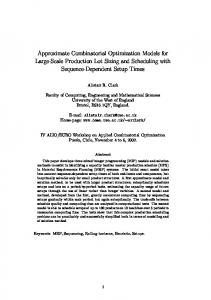
the parents of Xj , i.e., for each Xjk there is an edge pointing from Xjk to Xj . A Bayesian Q network represents the joint probability distribution given by: P (X) = nj=1 P (Xj |paj ). For example, consider a Bayesian network with 5 variables, whose directed acyclic graph (DAG) is given in Figure 1.1(a). Given a Bayesian network B = hX, D, P,

Q

i the most common optimization task is to find

the Most Probable Explanation (MPE), also known as Maximum A Posteriori hypotheQ sis (MAP). Its aim is to compute the maximum probability P ∗ = maxX f ∈P f and the Q corresponding assignment x∗ = arg maxX f ∈P f . Definition 1.4 (Markov network, [78],[21]). A Markov network is a graphical model T = Q hX, D, F, i, where F = {fS1 , . . . , fSr } is a set of functions, often referred to as potentials,

where each potential fSj is a non-negative real-valued function defined on scopes Sj ⊆ X. Q A Markov network represents the joint probability distribution given by: P (X) = Z1 rj=1 fj , P Qr where Z = X j=1 fj . The normalization constant Z is called the partition function, computing it is one of the main tasks over Markov networks.

10

P (A)

A

A

B

E

C

D

D

C

E

B

A

A

(c)

(d)

P (B|A)

B

C

B

C

P (C|A)

E

E

P (E|B, C)

D

D

P (D|A, B)

(a)

(b)

Figure 1.1: (a) A DAG of a Bayesian network, (b) its primal graph (also called moral graph), (c) its induced graph along o = (A, E, D, C, B), and (d) its induced graph along o = (A, B, C, D, E) (after [41]). Definition 1.5 (Weighted Constraint Satisfaction Problem, WCSP, [21]). WCSP is P a graphical model C = hX, D, F, i, where F = {fS1 , . . . , fSr } is a set of real-valued nonnegative functions. Each function fSj , also called cost-component, has a scope Sj ⊆ X and assigns ”0” (no penalty) to allowed tuples and a positive integer penalty cost to the forbidden tuples.

The primary optimization task over WCSP is finding a minimal cost assignment (min-sum): P P C ∗ = minx j fj (x) and the optimizing configuration x∗ = arg minx j fj (x). Histori-

cally this task is also sometimes referred to as energy minimization. It is equivalent to Q ∗ an MPE/MAP task in the following sense: if Cmax = maxx j fj (x) is a solution to an

∗ ∗ ∗ MPE problem, then Cmax = exp (−Cmin ), where Cmin is a solution to a min-sum problem P ∗ Cmin = minx j gj (x) and ∀j, gj (x) = − log (fj (x)).

A graphical model defines a primal graph capturing dependencies between the variables. Definition 1.6 (Primal graph). The primal graph of a graphical model is an undirected graph that has variables as its vertices. An edge connects any two variables that appear in the scope of the same function. 11

For a Bayesian network, the primal graph is also called a moral graph. Definition 1.7 (Moral graph). The moral graph of a directed graph is an undirected graph obtained by connecting all parents of a node to each other and removing direction.

Figure 1.1(b) depicts the primal graph of the Bayesian network in Figure 1.1(a). Note that parents of variable E (variables B and C) are connected in the primal graph. An important feature of a graphical model, that characterizes the complexity of its reasoning tasks, is the induced width. Definition 1.8 (Ordered graph, induced width ([21])). An ordered graph is a pair (G, o) where G is an undirected graph, and o = (X1 , . . . , Xn ) is an ordering of nodes. The width of a node is the number of the node’s neighbors that precede it in the ordering. The width of a graph along an ordering o is the maximum width over all nodes. An induced ordered graph is obtained from an ordered graph as follows: nodes are processed from last to first based on o; when node Xj is processed, all its preceding neighbors are connected. The width of an ordered induced graph along the ordering o is called induced width along o and is denoted by w∗ (o). The induced width of a graph, denoted by w∗ , is the minimal induced width over all its orderings. Abusing notation we sometimes use w∗ to denote the induced width along a particular ordering, when the meaning is clear from the context.

Figures 1.1(c) and 1.1(d) depict the induced graphs of the example primal graph in Figure 1.1(b) along the orderings o = (A, E, D, C, B) and o0 = (A, B, C, D, E), respectively. The dashed lines correspond to the induced edges, namely edges that are absent from the moral graph, but were introduced in the induced graph. The induced width along ordering o is w∗ (o) = 4 and the one along ordering o0 is w∗ (o0 ) = 2.

12

 1.2.2 Variable Elimination for Inference in Graphical Models Common approaches to solving optimization tasks over graphical models include variable elimination and conditioning algorithms, such as search (for details see [21]). In this section we present two schemes based on the variable elimination idea, leaving the discussion of search algorithms to Section 1.2.4.

 1.2.2.1 Exact Inference: Bucket Elimination Bucket elimination (BE) [19] is a framework that provides a unifying view of variable elimination algorithms for a variety of reasoning tasks. Algorithm 1 presents the bucket elimination algorithm for the MPE task. As an input it Q accepts a graphical model M = hX, D, F, i, a variable ordering o and a marginalization P operator max. For WCSP the combination operator is and the marginalization operator is min. Given a variable ordering, each variable is associated with a bucket constructed

as follows: all the functions defined on variable Xj , but not on variables appearing later in the ordering, are placed into the bucket of Xj . We denote the bucket of variable Xj as bucketXj or BXj . By Scope(BXj ) we denote the variables appearing in the functions in bucketXj . Namely, if BXj contains functions f1 , . . . , fk with scopes S1 , . . . , Sk respectively, then Scope(BXj ) = ∪kp=1 Sp . We say that the variable that appears later in the ordering o is a higher-index variable than the ones that appear sooner. Once the buckets are created, BE processes buckets from last to first. It computes new functions by combining all the functions in the bucket and then applying to the resulting function (known as the “bucket function”) the elimination operator (e.g., max). The newly computed functions, also called messages, are placed in lower buckets using the following rule. A function generated in BXj is placed in BXk , where Xk is the latest variable in Scope(BXj ) relative to ordering o, excluding Xj . We denote this function by hXj →Xk . This phase of 13

Algorithm 1: Bucket Elimination [19]

1 2

3 4

5 6

7 8

9

10

11

Q Input: Graphical model M = hX, D, F, i, variable ordering o, marginalization operator max Output: An optimal solution to the MPE task over M and the optimal assignment //Initialize Partition the functions in F into bucketX1 , . . . , bucketXn , where bucketXp contains all functions whose highest-index variable according to the ordering o is Xp ; //Backward pass for p ← n down to 1 do Let g1 , . . . , gr be the functions in bucketXp (including both original functions and previously generated messages) having scopes S1 , . . . , Sr , respectively; if Xp is instantiated (Xp = xp ) then Assign Xp = xp to each gj and put each resulting function into its appropriate bucket; else Q Generate the message function hXp →Xk : hXp →Xk = maxXp rj=1 gj , where Xk is the highest-index variable in Scope(hXp →Xk ) = ∪rj=1 Sj − Xp ; place hXp →Xk in bucketXk ;

//Forward pass Assign a value to each variable along ordering o which optimizes the combination of the functions currently in the bucket ; return The function computed in the bucket of the first variable and the corresponding assignment;

the algorithm is known as “the backward pass”. Subsequently, during the “forward pass”, the algorithm constructs a solution by assigning a value to each variable along the ordering, consulting the functions created during the backward phase. Note that the forward pass is relevant only to optimization tasks. For a summation task, such as finding the partition function, the algorithm bucket elimination would have only a backward pass. As an illustration we apply the bucket elimination algorithm to the network in Figure 1.1(a)

14

along o = (A, E, D, C, B), solving an MPE problem. We compute P ∗ as

P ∗ = max P (a, b, c, d, e)

(1.1)

a,b,c,d,e

= max P (a)P (c|a)P (e|b, c)P (d|a, b)P (b|a)

(1.2)

= max P (a) max max max P (c|a) max P (e|b, c)P (d|a, b)P (b|a).

(1.3)

a,b,c,d,e

a

e

d

c

b

Bucket elimination computes this expression from right to left using the buckets, as shown:

1. bucketB : hB→C (a, d, c, e) = maxb P (e|b, c)P (d|a, b)P (b|a) 2. bucketC : hC→D (a, d, e) = maxc P (c|a)hB→C (a, d, c, e) 3. bucketD : hD→E (a, e) = maxd hC→D (a, d, e) 4. bucketE : hE→A (a) = maxe hD→E (a, e) 5. bucketA : P ∗ = maxa P (a)hE→A (a),

A schematic trace of the algorithm is shown in Figure 1.2. Bucket elimination can be viewed as message passing from leaves to root along a so-called bucket tree, whose nodes are the buckets and bucketX is a child of bucketY , if there is a function hX→Y which is generated in bucketX and placed in bucketY during BE. The root bucket is often the first bucket. For example, the bucket tree of the problem in Figure 1.2 is a chain, since each bucket receives a message from only one other bucket. It was shown that, Theorem 1.1. [19, 21] Given a graphical model with variable ordering o having induced width w∗ (o), the time and space complexity of the bucket elimination scheme is O(r · k w O(n · k w

∗ (o)

∗ (o)+1

) and

) respectively, where r is the number of functions, n is the number of problem

variables and k is the maximum domain size. 15

max B

bucket B

P (E|B, C)

bucket C

P (C|A)

!

P (D|A, B)

P (B|A)

hB→C (A, D, C, E)

bucket D

hC→D (A, D, E)

bucket E

hD→E (A, E)

bucket A

P (A)

max

A,B,C,D,E

hE→A (A)

P (A, B, C, D, E)

Figure 1.2: A trace of bucket elimination algorithm Since the complexity of bucket elimination algorithm is exponential in induced width along the ordering, ideally we want to find a variable ordering that has the smallest induced width. Although this problem has been shown to be NP-hard [4], there are a few greedy heuristic algorithms that provide good orderings [20, 21].

 1.2.2.2 Approximate Inference: Mini-Bucket Elimination Bucket elimination is infeasible for many practical problems having large induced width. Thus an approximate version of the algorithm, called mini-bucket elimination (MBE) was proposed [25]. MBE (Algorithm 2) bounds the space and time complexity of the full bucket elimination. Given a variable ordering, the algorithm associates each variable Xk with a bucket, which contains all functions defined on this variable, but not on higher index variables, as bucket elimination does. Subsequently, when processing buckets, large buckets are partitioned into smaller subsets, called mini-buckets, each containing at most i + 1 distinct variables. The parameter i is called the i-bound. In the following we often use “i-bound” 16

Algorithm 2: Mini-Bucket Elimination [25]

1

2 3

4 5

6 7

8 9

10

11

12

Q Input: A graphical model M = hX, D, F, i, variable ordering o, marginalization operator max, parameter i Output: An approximate solution to the MPE task over M and an assignment to all variables //Initialize Partition the functions in F into bucketX1 , . . . , bucketXn , where bucketXp contains all functions whose highest-index variable is Xp . //Backward pass for p ← n down to 1 do Let g1 , . . . , gr be the functions in bucketXp (including both original functions and previously generated messages); let S1 , . . . , Sr be the scopes of functions g1 , . . . , gr ; if Xp is instantiated (Xp = xp ) then Assign Xp = xp to each gj and put each resulting function into its appropriate bucket; else Partition functions in BXp into mini-buckets, generating the partitioning QXp = {qp1 , . . . , qpl }, where each qpt ∈ QXp has no more than i + 1 variables; foreach qpt ∈ QXp do Q Generate the message function htXp →Xk = max Xp j gjt , where gjt ∈ qpt and Xk is the highest-index variable in Scope(htXp →Xk ) = ∪j Scope(gjt ) − Xp ; Add htXp →Xk to bucketXk ;

//Forward pass Assign a value to each variable in the ordering o so that the combination of the functions in each bucket is optimal, according to the marginalization operator max; return The function computed in the bucket of the first variable and the corresponding assignment;

and “i” interchangeably. We denote the mini-buckets obtained by partitioning the bucket BXp by QXp = {qp1 , . . . , qpn }, where qpj is the j th mini-bucket of variable Xp . MBE generates an upper bound on the optimal MPE/MAP value, Pˆ ≥ P ∗ (and lower bound on the optimal WCSP value). To demonstrate the execution of MBE we again turn to the network in Figure 1.1(a), with the ordering o = (A, E, D, C, B). Let us set i = 2, i.e., restrict each mini-bucket to contain no more than 3 variables. Since the scope of bucketB is greater than 3, it is necessary to split bucketB into two separate mini-buckets, which will then be processed independently. Let us assume that one of them contains function P (E|B, C) and the other functions P (D|A, B) 17

P (A)

P (A)

A

A

P (B|A)

P (B ′′ |A)

P (C|A)

B

C

B'

C

B''

P (C|A)

E D

E

P (E|B, C)

P (E|B ′ , C)

D P (D|A, B ′′ )

P (D|A, B) (a)

(b)

Figure 1.3: (a) The original Bayesian network, (b) The network with duplicated variable B and P (B|A). The question of how to best distribute the functions between mini-buckets is not trivial and is usually solved heuristically. More information can be found in [81]. Splitting bucketB into two mini-buckets can be viewed as replacing variable B by two duplicate variables: B 0 and B 00 . We denote the corresponding mini-buckets as bucketB 0 and bucketB 00 . Figure 1.3(a) shows the original network, and 1.3(b) presents the network with duplicated variables. Note that in Figure 1.3(b) variable A is no longer connected to B 0 , since no function has both these variables in its scope. An execution of MBE is equivalent to running an exact bucket elimination algorithm on the resulting modified problem1 :

1. bucketB 0 : hB 0 →C (c, e) = maxb P (e|b, c) 2. bucketB 00 : hB 00 →D (a, d) = maxb P (d|a, b)P (b|a) 3. bucketC : hC→E (a, e) = maxc P (c|a)hB 0 →C (c, e) 1 Notice also that the network in 1.3(b) is not fully legitimate as a Bayesian network since B 0 has no function. This however has no real consequence and will not be further discussed.

18

4. bucketD : hD→A (a) = maxd hB 00 →D (a, d) 5. bucketE : hE→A (a) = maxe hC→E (a, e) 6. bucketA : Pˆ = maxa P (a)hE→A (a)hD→A (a)

Figure 1.4 shows the trace of the mini-bucket elimination algorithm. max B

bucket B

!

bucket E bucket A

max

A,B ′ ,B ′′ ,C,D,E

B

!

P (D|A, B) P (B|A) ! "# $

P (E|B, C)

(C|A) bucket C P !

bucket D

max

hB ′ →C (C, E) "# $

hB ′′ →D (A, D)

hC→E (A, E) P (A) hE→A (A) hD→A (A) ! "# $

P (A, B ′ , B ′′ , C, D, E) ≥

max

A,B,C,D,E

P (A, B, C, D, E)

Figure 1.4: A trace of mini-bucket elimination algorithm Theorem 1.2. [25] Given a graphical model with variable ordering o having induced width w∗ (o) and an i-bound parameter i, the time complexity of the mini-bucket algorithm MBE(i) is O(n · k min(i,w

∗ (o))+1

) and space complexity is O(n · k min(i,w

∗ (o))

), where n is the number of

problem variables and k is the maximum domain size.

Higher values of i take more computational resources, but yield more accurate bounds. When i is large enough (i.e., i ≥ w∗ (o)), MBE coincides with the full bucket elimination.

19

As we will describe in greater details in Section 1.2.4.4, the mini-bucket elimination is often used to generate heuristics for both best-first and depth-first branch and bound search over graphical models [50, 51, 53].

 1.2.3 Heuristic Search Search algorithms are used in a vast variety of applications. Though we mostly concentrate on the application of search to optimization tasks over graphical models, we will provide some background on general purpose search schemes as well. For more information see, for example, Pearl [77]. Consider a search space defined implicitly by a set of states (the nodes in the graph), operators that map states to states, having costs or weights (the directed weighted arcs), a starting state n0 and a set of goal states. We say that a node is generated, when its representation code is computed based on the heuristic information and the information about its parent. It is said that the parent of the node is then explored, or expanded, when all its children have been generated. A node expansion consists of generating all successors of a given parent node. We call a path explored, if all nodes on this path have been expanded. The task typically assumed is to find the least cost solution path from n0 to a goal [72], where the cost of a solution path is the sum or the product of the weights on its arcs. Search procedure, or strategy, is a policy that determines the order, in which nodes are generated. We distinguish between blind (or uninformed ) search and informed (or heuristic) search. The former operates based only on information obtained during the search process (e.g., the cost of getting from the root to the current node). A heuristic search algorithm uses partial (heuristical) information about the search space and the goal in order to move towards more promising solutions. A heuristic function, denoted h(n), provides an estimate of the cost of the least cost path from each node n to any of 20

the goals. A heuristic function is called admissible, if and only if it never overestimates (for minimization task) the true minimal cost, h∗ (n), to reach the goal from node n, namely, ∀n h(n) ≤ h∗ (n). A heuristic is called consistent or monotonic, if for every node n and for every successor n0 of n we have:

h(n) ≤ c(n, n0 ) + h(n0 )

(1.4)

where c(n, n0 ) is the weight of the arc (n, n0 ). The two main heuristic search strategies are best-first search and depth-first branch and bound search. Both of them assess how promising each node is and make decisions concerning node expansions based on a numerical estimation called evaluation function, which estimates the minimal cost of the path from start to a goal that passes through node n.

 1.2.3.1 Best-First Search Best-first search (BFS) always expands the node with the best (e.g., smallest for minimization problem) value of the evaluation function. It maintains a graph of explored paths, a list CLOSED of expanded nodes and a frontier of OPEN nodes. BFS chooses from OPEN a node n with lowest value of an evaluation function f (n), expands it, places it on CLOSED, and places its child nodes on OPEN. The most popular variant of best-first search, A*, uses the evaluation function f (n) = g(n) + h(n), where g(n) is the current minimal cost from the root to n, and h(n) is a heuristic function that estimates the optimal cost-to-go h∗ (n) from n to a goal node. In the following we assume that the heuristic used by A* is admissible, unless specified otherwise. If h(n) is consistent, then the values of evaluation function f (n) along any path are non-decreasing. A path π is called C ∗ -bounded relative to f , if ∀n ∈ π : f (n) < C ∗ , where C ∗ is the cost of optimal solution. It is known that, regardless of the tie-breaking rule, A* expands any node n that is reachable by a strictly 21

C ∗ -bounded path from the root. Such a node is said to be surely expanded by A* [24]. A* search possesses a number of attractive properties [72, 77, 24]:

• Soundness and completeness: A* terminates with an optimal solution. • When h is consistent, A* explores only the nodes in the set S = {n|f (n) ≤ C ∗ } and it surely expands all the nodes having S = {n|f (n) < C ∗ }. • Optimal efficiency under consistent heuristic: When h is consistent, any node surely expanded by A* must be expanded by any other sound and complete search algorithm having access to the same heuristic information. Also, in thise case A* will expand each node at most once, when searching a graph, because at the time of node’s expansion A* has found the least-cost path to it. • Dominance: Given two heuristic functions h1 and h2 , such that ∀n h1 (n) < h2 (n), A∗1 will expand every node surely expanded by A∗2 , where A∗j uses heuristic hj .

Though best-first search is known to be the best algorithm in terms of number of nodes expanded [24], sometimes it requires storing the whole search space, which means often an exponential memory in the worst-case.

 1.2.3.2 Depth-First Branch and Bound A popular alternative is depth-first branch and bound (DFBB), whose most attractive feature, compared to best-first search, is that it can be executed with linear memory. Yet, when the search space is a graph, it can exploit additional memory to improve its performance by flexibly trading space and time. Depth-first branch and bound expands nodes in a depth-first manner, maintaining an upper bound U B on the cost of the optimal solution, which equals to the best solution cost found 22

(a) Primal graph

(b) OR search tree along ordering A, B, C, D, E, F

Figure 1.5: OR search space example problem (after [75]) so far (initially infinity). If the evaluation function of the current node n is greater than the upper bound, the node is pruned and the subtree below it is never explored. In the worst case depth-first branch and bound explores the entire search space. In the best case the first solution found is optimal, in which case DFBB’s performance can be as good as BFS. However, if the solution depth is unbounded, depth-first search might follow an infinite branch and never terminate. Also, if the search space is a graph, DFBB may expand nodes numerous times, unless it uses additional memory for caching and checks for duplicates. The average case is hard to characterize for both DFBB and BFS because we do not know C ∗ , and even if we did, we cannot easily estimate the set {n|f (n) ≤ C ∗ }. This depends on the values of heuristic function and, for DFBB, on the order in which the solutions are encountered.

 1.2.4 Heuristic Search in Graphical Models Search algorithms provide a way to systematically enumerate all possible assignments of a given graphical model. Optimization problems can be naturally presented as the task of finding an optimal cost path in an appropriate search space. The simplest variant of a search space is a so-called OR search tree. Each level of this tree corresponds to a variable from the original problem. The nodes correspond to variable 23

assignments and the arc weights are derived from problems’ functions. The size of such search tree is O(k n ), where n is the number of variables and k is the maximum domain size. Throughout this section we illustrate the concepts using the example problem with six variables (A, B, C, D, E, F ) and seven pairwise functions. Its primal graph is shown in the Figure 1.5(a). Figure 1.5(b) displays the corresponding OR search tree along lexicographical ordering (after [75]).

 1.2.4.1 AND/OR Search Spaces OR search trees are blind to the problem decomposition encoded in the graphical models and can therefore be inefficient. They do not exploit the independencies in the model. AND/OR search spaces for graphical models have been introduced to better capture the problem structure [23]. The AND/OR search space is defined by a pseudo-tree of the primal graph that captures problem decomposition. Definition 1.9 (Pseudo-tree, [36]). A pseudo-tree of an undirected graph G = (V, E) is a directed rooted tree T = (V, E 0 ), such that every arc of G not included in E 0 can be viewed as a back-arc relative to T , namely it is an arc that connects a node to an ancestor relative to T . A node n0 is an ancestor of n in T if it appears on the path from the root to n in T . Definition 1.10 (AND/OR search tree, [23]). Given a graphical model M = hX, D, F,

N i

with primal graph G and a pseudo-tree T of G, the AND/OR search tree ST contains alter-

nating levels of OR and AND nodes. Its structure is based on the underlying pseudo-tree T . The root node of ST is an OR node labelled by the variable at the root of T . The children of an OR node labeled Xj are AND nodes labelled with value assignments hXj , xj i (or simply hxj i); the children of an AND node hXj , xj i are OR nodes labelled with the children of Xj in T , representing conditionally independent subproblems. Figure 1.6(a) shows a pseudo-tree of the example problem. The solid directed edges belong 24

A

OR

A

AND

0

1

OR

B

B

B

AND

C

0

1

0

1

E C

OR AND

D

F

E

C

C

E

E

1

0

1

0

1

0

1

0

1

0

1

0

1

0

1

D D

F

F

D D

F

F

D D

F

F

D D

F

F

0

OR

C

E

AND 0 1 0 1 0 1 0 1

0 1 0 1 0 1 0 1

0 1 0 1 0 1 0 1

0 1 0 1 0 1 0 1

(a) Pseudo-tree (b) AND/OR search tree A

OR AND

0

1

OR

B

B

AND

0

C

C

OR AND

1

0

1

0

0

C

C 1

0

1

0

1

E 1

0

E 1

0

E

E 1

0

1

0

1

OR

D

D

D

D

F

F

F

F

AND

0 1

0 1

0 1

0 1

0 1

0 1

0 1

0 1

(c) Context-minimal AND/OR search graph

Figure 1.6: AND/OR search spaces example to the pseudo-tree. The dashed lines represent the back-arcs in the primal graph depicted in Figure 1.5(a), but are not part of the pseudo-tree. An AND/OR tree corresponding to the pseudo-tree in Figure 1.6(a) is shown in Figure 1.6(b). The arcs from nodes Xj to hXj , xj i in an AND/OR search tree are annotated by weights that are derived from the cost functions in F as follows. Definition 1.11 (Arc weight, [23]). The weight w(Xj , xj ) of the arc (Xj , hXj , xj i) is the combination (i.e., sum for WCSP and product for MPE) of all the functions, whose scope 25

includes Xj and which are fully assigned by values specified along the path from root to the node to hXj , xj i. Theorem 1.3. [23] Given a pseudo-tree T of a graphical model having height h, the size of the AND/OR search tree based on T and the time complexity of an algorithm exploring it are bounded by O(n · k h ), where n is the number of variables and k bounds their domain size. Definition 1.12 (Context, [23]). Given the primal graph G = (V, E) of a graphical model M and a corresponding pseudo-tree T , the context of a node Xj (referred to originally as OR context) in T is the set of the ancestors of Xj in T that have connections in G to Xj or its descendants.

In other words, the context of a variable Xj is a set of variables, for which any partial instantiation separates the subproblem rooted at Xj from the rest of the network. When talking about the context of a subproblem, we imply the context of the subproblem’s root node. Definition 1.13 (Context-minimal AND/OR search graph, [23]). A context-minimal AND/OR search graph, denoted CT , is obtained from an AND/OR search tree by merging all the identical subproblems that have the same context. Theorem 1.4. [23] Given a graphical model M = hX, D, F,

N i with a primal graph G,

whose induced width along the pseudo-tree T is w∗ , the size of a context-minimal AND/OR ∗

search graph is O(n · k w ). Definition 1.14 (Solution tree, [65]). A solution tree T of a context-minimal AND/OR search graph CT is a subtree such that: (1) it contains the root node of CT ; (2) if an internal AND node n is in T , then all its children are in T ; (3) if an internal OR node n is in T , then exactly one of its children is in T ; (4) every tip node in T (i.e., node with no children, also known as leaf node) is a terminal node, namely it has no children in CT . 26

Definition 1.15 (Cost of a solution tree, [65]). The cost of a solution tree is the product (for MPE task) or sum (for WCSP) of the weights associated with its arcs (not to be confused with computational cost of the tree construction, namely its time and space complexity).

Each node n in CT is associated with a value v(n) capturing the optimal solution cost of the conditioned subproblem rooted in n. Assuming an MPE/MAP problem, it was shown that v(n) can be computed recursively based on the values of n’s successors: OR nodes by maximization and AND nodes by multiplication. In the case of WCSPs, v(n) for OR and AND nodes is computed as a function of their child nodes by minimization and summation, respectively [23]. We next provide an overview of a depth-first branch and bound and a best-first search algorithms that explore AND/OR search spaces [69, 68, 76]. These schemes use heuristics generated either by the mini-bucket elimination scheme (see Section 1.2.4.4 for details) or through soft arc-consistency schemes [68, 69, 83, 16] or their composite [48]. As is customary in the heuristic search literature, when defining algorithms we assume without loss of generality a minimization task (i.e., min-sum optimization problem).

 1.2.4.2 AND/OR Best-First Search The state-of-the-art version of A* for the AND/OR search space for graphical models is the AND/OR Best-First algorithm (AOBF) [69]. AOBF is a variant of AO* [72] that explores the AND/OR context-minimal search graph. AOBF (Algorithm 3) maintains the explicated part, denoted G, of the context-minimal AND/OR search graph CT , namely all the nodes of CT that AOBF generated so far and the edges between them. It also keeps track of the current best partial solution tree T ∗ . AOBF interleaves iteratively a top-down node expansion step (lines 4-16), selecting a non-terminal tip node of T ∗ and generating its children in the explored search graph G, with a bottom27

Algorithm 3: AOBF(hi ) exploring AND/OR search tree [69]

1 2 3 4

5 6 7 8 9 10

11 12 13 14

15 16

17 18 19 20

21 22 23 24 25 26 27 28 29

P Input: A graphical model M = hX, D, F, i, pseudo-tree T rooted in X1 , heuristic hi calculated with i-bound i; Output: Optimal solution to M create root OR node s labelled by X1 and let G (explored search graph) = {s}; initialize v(s) = hi (s) and best partial solution tree T ∗ to G; while s is not SOLVED do select non-terminal tip node n in T ∗ . If there is no such node then exit; // expand node n if n = Xj is OR then forall the xj ∈ D(Xj ) do create AND child n0 = hXj , xj i; if n’ is TERMINAL then mark n0 SOLVED; succ(n) ← succ(n) ∪ n0 ; else if n = hXj , xj i is AND then forall the successor Xk of Xj in T do create OR child n0 = Xk ; succ(n) ← succ(n) ∪ n0 ; initialize v(n0 ) = hi (n0 ) for all new nodes; add new nodes to the explored search space graph G ← G ∪ succ(n); // update n and its AND and OR ancestors in G, bottom-up repeat if n is OR node then v(n) = mink∈succ(n) (w(n, k) + v(k)); mark the best successor k of OR node n, such that k = arg mink∈succ(n) (w(n, k) + v(k)) (maintaining previously marked successor if still the best); mark n as SOLVED if its best marked successor is solved; else if n isPAND node then v(n) = k∈succ(n) v(k); mark all arcs to the successors; mark n as SOLVED if all its children are SOLVED; n ← p; //p is a parent of n in G until n is not root node s; recompute T ∗ by following marked arcs from the root s; return hv(s), T ∗ i;

up cost revision step (lines 17-27), updating the values of the internal nodes based on the children’s values. If a newly generated child node is terminal, it is marked solved (lines 8-9). During the bottom-up phase the OR nodes having at least one solved child and the AND nodes having all children solved are also marked as solved (lines 21 and 25). AOBF also marks the arc to the best AND child of an OR node, through which the minimum is achieved (line 20). After the bottom-up step, a new best partial solution tree T ∗ is recomputed (line 28

28). AOBF terminates when the root node is marked solved. For admissible heuristic at termination T ∗ is the optimal solution tree with the cost v(s), where s is the root node of the search space. Theorem 1.5. [69] The AND/OR Best-First search algorithm traversing the context-minimal ∗

AND/OR graph has the time and space complexity of O(nk w ), where n is the number of variable in the problem, w∗ is the induced width along the pseudo-tree and k bounds the domain size.

 1.2.4.3 AND/OR Depth-First Branch and Bound The AND/OR Branch and Bound [68] algorithm traverses the context-minimal AND/OR graph in a depth-first rather than best-first manner, while keeping track of the current upper bound on the minimal solution cost. The algorithm (Algorithm 4) interleaves forward node expansion (lines 4-17) with a backward cost revision (or propagation) step (lines 19-29) that updates node values (capturing the current best solution to the subproblem rooted at each node), until search terminates and the optimal solution is found. A node n is pruned (lines 12-13) if the current upper bound on the best solution rooted in n is higher than the heuristic lower bound, computed recursively using the procedure described in Algorithm 5. Theorem 1.6. [66] The worst case time and space complexity of AND/OR Branch and Bound exploring a context-minimal AND/OR search graph of a graphical model with n vari∗

ables, maximum domain size k, and an induced width w∗ along the pseudo-tree T is O(nk w ). In practice AOBB is likely to expand more nodes than AOBF using the same heuristic, but empirical performance of AOBB depends heavily on the order, in which the solutions are encountered, namely on how quickly the algorithm finds an optimal solution, that it will use as an upper bound for pruning. 29

Algorithm 4: AOBB(hi ) exploring AND/OR search tree [69] 1 2 3 4 5 6 7 8 9 10 11 12 13

P Input: A graphical model M = hX, D, F, i, pseudo-tree T rooted at X1 , heuristic hi ; Output: Optimal solution to M create root OR node s labelled by X1 and let stack of created but not expanded nodes be OPEN = {s}; initialize v(s) = ∞ and best partial solution tree rooted in s T ∗ (s) = ∅; U B = ∞; while OPEN6= ∅ do select top node n on OPEN. //EXPAND if n is OR node labelled Xj then foreach xj ∈ D(Xj ) do //Expand node n: add AND child n0 = hXj , xj i to list of successors of n; initialize v(n0 ) = 0, best partial solution tree rooted in n T ∗ (n0 ) = ∅; if n is AND node labelled hXj , xj i then foreach OR ancestor p of n do recursively evaluate the cost of the partial solution tree rooted in p, based on heuristic hi , assign its cost to f (p); // see evalPartialSolutionTree(Tn∗ , hi (n)) in Algorithm 5 if evaluated partial solution is not better than current upper bound at p (e.g., f (p) ≥ v(p) for minimization) then prune the subtree below the current tip node n; else

14

foreach successor Xk of Xj ∈ T do add OR child n0 = Xk to list of successors of n; initialize v(n0 ) = ∞, best partial solution tree rooted in n T ∗ (n0 ) = ∅;

15 16 17

18

19 20 21 22 23 24 25 26 27 28

29 30

add successors of n on top of OPEN; //PROPAGATE //Only propagate if all children are evaluated and the final v are determined while list of successors of node n is empty do if node n is the root node then return solution: v(n), T ∗ (n) ; else //update ancestors of n, AND and OR nodes p, bottom up: if p is AND node then v(p) = v(p) + v(n), T ∗ (p) = T ∗ (p) ∪ T ∗ (n); else if p is OR node then vnew (p) = w(p, n) + v(n); if the new value of better than the old one (e.g., vnew (p) > (w(p, n) + v(n)) for minimization then v(p) = vnew (p), T ∗ (p) = T ∗ (p) ∪ hxj , Xj i; remove n from the list of successors of p; move one level up: n ← p;

Breadth Rotating AND/OR Branch and Bound (BRAOBB). AOBB, though shown to be a powerful search scheme for graphical models, however, lacks a proper anytime behavior: at each AND node all but one independent child subproblems have to be solved completely, before the last one is even considered. To remedy this the Breadth-Rotating AND/OR Branch and Bound algorithm has been introduced recently [76]. The basic idea is to rotate through different subproblems in a breadth-first manner. The

30

Algorithm 5: Recursive computation of the heuristic evaluation function [69]

1 2 3 4 5 6 7 8 9

function evalPartialSolutionTree(Tn0 , h(n)) Input: Partial solution subtree Tn0 rooted at node n, heuristic function h(n); Output: Heuristic evaluation function f (Tn0 ); if succ(n) == ∅ then return h(n); else if n is an AND node then let k1 , . . . , kl be the OR children of n; Pl return j=1 evalPartialSolutionTree(Tk0 j , h(kj ));

else if n is an OR node then let k be the AND child of n; return c(n, k) + evalPartialSolutionTree(Tk0 , h(k));

concepts is illustrated in Figure 1.7. In Figure 1.7(a) the two subproblems on the left have been solved completely before the subproblem on the right was even considered. In Figure 1.7(b) the initial solutions to the three independent subproblems are found in parallel. As an input parameter the algorithm has a threshold z, defining the limit on the number of nodes expanded before switching to the next subproblem. Algorithm 6 shows the pseudo-code of BRAOBB. As mentioned above, the main difference between this algorithm and AOBB lies in the rotation of the subproblems. The subproblems are added into a global queue (GLOBAL), that insures that they are processed in a breadthfirst manner. Each individual subproblem is explored as usual in a depth-first manner, using the stack LOCAL for the current subproblem. In the beginning there is only one subproblem, rooted in the first variable X1 in the GLOBAL queue (line 3). As long as there are still subproblems in the GLOBAL queue, the next subproblem is taken from the queue and put on the LOCAL stack (line 6). The subproblem is then processed (lines 7-26) until either LOCAL becomes empty, i.e., the current subproblem is fully solved, or the number of nodes expanded reaches the threshold z, or the current subproblem decomposes further. In the latter case the new subproblems are added to queue GLOBAL for subsequent processing (lines 27-28). 31

processing

solved optimally

rotate (b)

(a)

Figure 1.7: Illustration of subproblem processing: (a) default by AOBB, (b) subproblem rotation by BRAOBB Empirically, BRAOBB was shown to find the first suboptimal solution significantly faster than plain AOBB [76].

 1.2.4.4 Mini-Bucket Heuristics The AND/OR search algorithms presented (AOBF, AOBB and BRAOBB) most often use the mini-bucket (also known as MBE ) heuristic h(n), formulated for OR search spaces by Kask [50, 51, 53] and extended for AND/OR search by Marinescu [66]. As shown in [66], the intermediate bucket functions generated by MBE(i) underestimate the optimal solution cost to subproblems rooted in each node of the AND/OR search graph (assuming a minimization query), just as the overall bound returned by MBE(i) is a lower bound on the overall solution. These intermediate functions can therefore be used to derive a heuristic function that is admissible. 32

Algorithm 6: BRAOBB(hi ) 1 2 3 4 5 6

7 8 9 10 11 12 13 14 15 16 17 18 19 20 21 22 23

24 25 26

P Input: A graphical model M = hX, D, F, i, pseudo-tree T rooted at X1 ; heuristic hi , rotation threshold Z; Output: Optimal solution to M Create root OR node s labelled by X1 (generate root subproblem) Initialize U B = ∞ GLOBAL←[ROOT] //put the root subproblem into queue while GLOBAL6= ∅ do //next subproblem for z from 1 to Z or until LOCAL is empty or until childSubprom(LOCAL)6= ∅ do n ←top(LOCAL); //next node in subproblem // Expand node n: if n is OR node labelled Xj then foreach xj ∈ D(Xj ) do initialize AND child n0 = hXj , xj i as in AOBB (line 7); add it on top of LOCAL; if n is AND node labelled hXj , xj i then foreach OR ancestor m of n do evaluate the heuristic and prune like in AOBB (lines 10-13); if no pruning happened then Y1 , . . . , Yk ← children of n in the pseudo-tree; generate OR children of hY1 i, . . . , hYk i ; if k=1 then //if there is no decomposition push Y1 to top of LOCAL; else if k > 1 then //problem decomposition for r ← 1 to k do NEW ← {hYr i}; //new child subproblem push NEW to the back of GLOBAL;

if children(n)6= ∅ then //if n is a leaf do propagation as in AOBB (lines 18-30); //upward in search space

28

if LOCAL6= ∅ then //subproblem is not yet solved push LOCAL to the end of GLOBAL;

29

return value(root) //root node has optimal solution

27

Recently more advanced heuristics for AND/OR search, such as mini-bucket elimination with max-marginal-matching and Joint Graph Linear Programming have been proposed [48]. We will discuss them and evaluate their performance in Chapters 5. Having established the necessary background, we will now turn to the main part of the thesis, presenting our contributions.

33

Chapter 2

Bucket Elimination for M -best Optimization Task

 2.1 Introduction1 The usual aim of combinatorial optimization is to find an optimal solution, minimum or maximum, of an objective function. However, in many applications it is desirable to obtain not just a single optimal solution, but a set of the first m best solutions for some integer m. We are motivated by many real-life domains, in which such task arises. For instance, the problem of finding the most likely haplotype in a pedigree can be presented as finding the most probable assignment in a Bayesian network that encodes the genetic information [34]. In practice the data is often corrupted or missing, which makes the single optimal solution unreliable. It is possible to increase the confidence in the answer by finding a set of m best solutions and then choosing the final solution with an expert help or by obtaining additional genetic data. More examples of the m-best task arise in procurement auction problems and in probabilistic expert systems, where certain constraints often cannot be directly incorporated into the model, either because they make the problem infeasibly complex or they are too 1

Part of this work has already been published in Natalia Flerova, Emma Rollon, and Rina Dechter. ”Bucket and mini-bucket Schemes for M Best Solutions over Graphical Models”, Special Issue of Lecture Notes in Computer Science: Graph structures for knowledge representation and reasoning, 2011.

34

vague to formalize (e.g., idiosyncratic preferences of a human user). Thus in such domains it may be more practical to first find several good solutions to a relaxed problem and then pick the one that satisfies all additional constraints in a post-processing manner. Additionally, sometimes a set of diverse assignments with approximately the same cost is required, as in reliable communication network design. Finally, in the context of a summation problem, such as probability of evidence or finding the partition function, an approximation can be derived by summing over the m most likely tuples, though we do not expect this bound to be tight in practice. The problem of finding the m best solutions has been well studied. One of the earliest and most influential works belongs to Lawler [61]. He provided a general scheme that extends any optimization algorithm to the m-best task. The idea is to compute the next best solution successively by finding a single optimal solution for a slightly different reformulation of the original problem that excludes the solutions generated so far. This approach has been extended and improved over the years and is still one of the primary strategies for finding the m best solutions. Other approaches are more direct, trying to avoid the repeated computation inherent to Lawler’s scheme. Two earlier works, that are most relevant and provide the highest challenge to our work, are by Nilsson [73] and Aljazzar, et al., [2].

• Nilsson [73] proposed a junction-tree-based message-passing scheme that iteratively finds the m best solutions. He claimed that it has the best runtime complexity among m-best schemes for graphical models. Our analysis (Section 3.5) shows that indeed Nilsson’s scheme has the second best worst case time complexity after our algorithm BE+m-BF (Section 3.4.3). However, in practice this scheme is often not feasible for problems having a large induced width. • Aljazzar, et al., [2] proposed an algorithm called K*, an A* search-style scheme for finding the k shortest paths, that is interleaved with breadth-first search. They used a very 35

specialized data structure, and it is unclear if this approach can be straightforwardly extended to graphical models, a point that we will leave to future work.

One of the popular approximate approaches to solving optimization problems is based on an LP-relaxation of the problem [99]. The m-best extension of this approach [37] does not guarantee exact solutions, but is quite efficient in practice. We will discuss these and other related works further in Chapter 3, in Section 3.5. Our main focus lies in optimization in the context of graphical models, such as Bayesian networks, Markov networks and constraint networks. However, some of the algorithms developed can be used for more general tasks, such as finding m shortest paths in a graph. Various graph-exploiting algorithms for solving optimization tasks over graphical models were proposed in the past few decades. Such algorithms are often characterized as being either of inference type (e.g., message-passing schemes, variable elimination) or of search type (e.g., AND/OR search or recursive-conditioning). In this chapter we limit our treatment to the class of inference schemes, as represented by the bucket elimination algorithm (BE) [19]. The discussion of search schemes is deferred till Chapter 3. Our contribution. We will show that the extension of the bucket elimination to compute the m-best solutions can be achieved by a relatively simple modification of its underlying combination and marginalization operators [19]. In optimization tasks over probabilistic graphical models the combination operator is a product, while the marginalization operator is maximization or minimization (we assume maximization here). We will show that the extension of the bucket elimination algorithm for the m-best solutions can be facilitated by representing functions as vector functions, by defining the combination operator to be a product between vector functions and the marginalization operator as m-sorting (rather than maximization). Applying these modifications yielding the bucket-elimination algorithm elimm-opt is described within the framework of semirings [85, 1, 56, 7]. This unifying formulation 36

ensures the soundness and completeness of any algorithm applied to any problem that fits into the framework and in particular it implies that elim-m-opt solves the m-best optimization task. We show that the worst-case complexity of our algorithm increases by a factor of O(m·log(m· deg)) over finding a single best solution, where deg is the highest degree of the bucket-tree ∗

that underlies the computation. This yields an overall complexity of O(m·n·k w ·log(m·deg)) when m is the number of solutions, n is the number of variables in the problem, k bounds the domain size of each variable and w∗ bounds the induced-width of the graphical model. Since the bucket elimination scheme can be approximated by the relaxation and bounding scheme of mini-bucket elimination (MBE) [25], we can extend elim-m-opt straightforwardly to a mini-bucket scheme mbe-m-opt, which computes a bound on each of the m best solutions. More significantly, we also show that the m bounds computed by mbe-m-opt can be used to tighten the bound on the first best solution, since both are generated from the same relaxed problem. In particular, it can facilitate a scheme for tightening any heuristic generation scheme. The formulation of the m-best problem using semiring framework makes a variety of schemes immediately applicable to this task, such as the Generalized Distributive Law [1] and Iterative Join-Graph Propagation [22]. The remainder of the chapter is organized in the following manner. In Section 2.2 we give the background on the semirings framework and more formally re-define in the context of semirings the combination and marginalization operators, as well as the reasoning task over graphical models, previously introduced in Section 1.2.1.2. We also axiomatically state the correctness of the bucket elimination algorithm, based on the results by Shenon and Shafer [88, 87]. Section 2.3 presents the formulation of the m-best reasoning task in the semiring framework. In Section 2.4 we describe the extension of bucket elimination algorithm to the 37

m-best. Section 2.5 is devoted to the extension of mini-bucket elimination to the m-best task. Section 2.6 presents empirical evaluation. Section 2.7.

 2.2 Preliminaries and Background Before moving on to our main contributions, in this section we give more formal definitions of some graphical models concepts previously presented in Section 1.2.1.2 and axiomatically describe the properties of the algorithms for solving the reasoning tasks over graphical models. Most of the results are based on the works of Shenon and Shafer [88, 87] and Bistarelli, et al., [8]. Though some of the definitions included in this section may seem familiar from the previous chapter, the mathematically formal formulations presented here are crucial for proving the correctness of the new m-best algorithm we introduce in Section 2.4. As before, let X = {X1 , . . . , Xn } be an ordered set of variables and D = {D1 , . . . , Dn } an ordered set of domains. Domain Dj is a finite set of potential values for Xj . Let us denote the assignment (i.e., instantiation) of variable Xj with xj ∈ Dj as Xj = xj . A tuple is an ordered set of assignments to different variables (X1 = x1 , . . . , Xk = xk ). A complete assignment is an assignment to all variables in X. Let t and s be two tuples having the same instantiations to the common variables. Their join, noted t · s, is a new tuple which contains the assignments of both t and s. We use the symbol · for both join and multiplication, however, the context usually makes the meaning unambiguous. Definition 2.1 (Field, valuations). A field is an algebraic structure with notions of addition, subtraction, multiplication, and division, satisfying certain axioms. A valuation is a function on the elements of a field that provides a measure of size or multiplicity of elements of the field.

Alternatively, we can define valuations the following way. Let the scope of a function f be 38

Y. For a subset of variables Y, we denote by DY the set of tuples over Y, namely the set of all possible assignments to variables in Y. Let f : DY → A be a function having scope Y, A is a set of valuations. When the correspondence between valuations and variable sets can be ambiguous, we more specifically talk about valuations on Y denoted AY . Typical ranges of valuations A are natural, real and boolean numbers. For example, in the case of Bayesian networks a valuation is a set of non-negative, real-valued numbers. For each set of valuations A there can be at most one valuation ζ ∈ A called a zero valuation. In case of a Bayesian network the zero valuation is such valuation ζ that the values of the function f : DY → ζ are zero for all configurations of Y. For a subset of variables Y and function f : DY → A a subset of valuations P ∈ A is called proper valuations if P = A \ ζ, where ζ is a zero valuation. The notion of proper valuations is important, as it will enable us to define combinability of valuations. In the probability case, a valuation A is said to be proper if the values of the function DY → A are not zero for all configurations of Y. We assume two binary operations over valuations: ⊗ : A × A → A called combination (or multiplication) and ⊕ : A × A → A called addition or marginalization. Both operators are associative and commutative. Following [88] we define these operators in the following way: Definition 2.2 (Combination). We assume there is a mapping ⊗ : A × A → A, called combination, such that:

1. If GY and HZ are valuations on Y and Z, then GY ⊗ HZ is a valuation on Y ∪ Z; 2. If either GY or HZ is not a proper valuation, then GY ⊗ HZ is not a proper valuation; 3. If GY and HZ are both proper valuations, then GY ⊗ HZ may or may not be a proper valuation.

39

If GY ⊗ HZ is not a proper valuation, then we shall say that GY and HZ are not combinable. If GY ⊗ HZ is a proper valuation, then we shall say that GY and HZ are combinable and that GY ⊗ HZ is the combination of GY and HZ . As was pointed out in [88], intuitively, combination corresponds to aggregation. If GY and HZ represent information about variable sets Y and Z, respectively, then GY ⊗ HZ represents the aggregated information for variables in Y ∪ Z. In the Bayesian networks case, combination corresponds to multiplication. Definition 2.3 (Marginalization or addition). We assume that for each subset of variables Y and subset Z ⊆ Y there is a mapping ⊕Z : A × A → A, called marginalization to Z, such that

1. If GY is a valuation on Y and Z ⊆ Y, then ⊕Z GY is a valuation on W, where W = Y \ Z is a relative complement of a set Z with respect to a set Y, namely the set of elements in Y, but not in Z; 2. If GY is a proper valuation, then ⊕Z GY is a proper valuation; 3. If GY is not a proper valuation, then ⊕Z GY is not a proper valuation. Intuitively, marginalization corresponds to narrowing the focus of a valuation. If GY is a valuation on Y representing some information about variables in Y, and Z ⊆ Y, then ⊕Z GY represents the information for variables in Y implied by GY , if we disregard variables in Y \ Z. [88]. In the belief network case the marginalization corresponds to summation. Definition 2.4 (Valuation structure). A valuation structure is a triple K = (A, ⊗, ⊕) such that A is an arbitrary set of valuations.

In order to be able to formally define the reasoning task and discuss the algorithms which can solve it we extend the combination and addition operators to operate also over functions. 40

Definition 2.5 (Combination operator over functions). Let fSj : Dj → A and gSp : N Dp → A be two functions. Their combination, noted fSj gSp relative to A, is a new function hSk with scope Sk = Sj ∪Sp , which returns for each tuple t ∈ DSj ∪Sp the combination of valuations of fSj and gSp . Formally,

∀t ∈ Dh , hk (t) = fj (t) ⊗ gp (t) In the framework of graphical models combination operator ⊗ is defined by enumeration as Q P ⊗ ∈ { , , ./}.

Definition 2.6 (Marginalization operator over functions). Let fSj : Dj → A be a

function and W ⊆ X be a set of variables. The marginalization of W from fSj , noted fSj ⇓W relative to A, is a new function hSk with the scope Sk = Sj \ W that returns for each tuple t ∈ DSj −W the addition of the valuations over the different extensions to W. Formally, ∀t ∈ Dk , hSk (t) = ⊕t0 ∈DW fSj (t · t0 ) In the framework of graphical models marginalization operator ⇓ is defined by enumeration Q P as ⇓= {max, min, , }.

Example 2.1. For example, consider three variables X1 , X2 and X3 with domains D1 = D2 = D3 = {1, 2, 3}. Let f (X1 , X2 ) = X1 X2 and g(X2 , X3 ) = 2X2 + X3 be two functions. If

the combination operator is product (i.e., ·), then (f × g)(X1 , X2 , X3 ) = X1 X2 · (2X2 + X3 ). If the marginalization operator is max, then (f ⇓X1 )(X2 ) = max {1X2 , 2X2 , 3X2 } = 3X2 . For completeness we re-state here the previously given definition of the graphical model and the reasoning task, keeping in mind that they assume the new, more mathematically strict, definitions of the combination and marginalization operators. Definition 2.7 (Graphical model). A graphical model is a tuple M = hX, D, A, F, 41

N i,

where: X = {X1 , . . . , Xn } is a set of variables; D = {D1 , . . . , Dn } is the set of their finite domains of values; A is a set of valuations (A, ⊗, ⊕); F = {f1 , . . . , fr } is a set of N discrete functions, where var(fj ) ⊆ X and fj : Dfj → A; and is the combination operator over functions (see Definition 2.5). The graphical model M represents the function N C(X) = f ∈F f .

N Definition 2.8 (Reasoning task). A reasoning task is a tuple P = hX, D, A, F, , ⇓i N where hX, D, A, F, i is a graphical model and ⇓ is a marginalization operator over functions as defined in Definition 2.6. The reasoning task is to compute F (X) ⇓X .

N For a reasoning task M = (X, D, A, F, , ⇓) the choice of (A, ⊗, ⊕) determines the comN bination and marginalization ⇓ operators over functions, and thus the nature of the graphical model and its reasoning task. For example, if A is the set of non-negative reals N and is product, the graphical model is a Markov network or a Bayesian network. If ⇓ is max, the task is to compute the Most Probable Explanation (MPE), while if ⇓ is sum, the task is to compute the Probability of the Evidence. The correctness of the algorithmic techniques for computing a reasoning task relies on the properties of the set of valuations and the combination and marginalization operators. These properties are axiomatically described by means of an algebraic structure over (A, ⊗, ⊕). In other words, reasoning tasks on graphical models can be axiomatically described. As a result, any new problem expressed in that axiomatization immediately inherits the techniques developed for the existing ones. Two main axiomatizations proposed in the literature are the Shenoy-Shafer [88] and the semiring CSP framework [9]. In the first one, the triplet (A, ⊗, ⊕) is a commutative semiring, while in the second one, the triplet (A, ⊗, ⊕) is a so-called c-semiring, that is, a commutative semiring with ⊕ being idempotent. While Shenoy and Shafer focus in their work mainly on 42

the tasks over belief networks, Bistarelli, et al., [9] propose SCSP (Semiring CSP), a general framework for constraint satisfaction problems, that provide unification for classical CSPs, fuzzy CSPs, weighted CSPs, partial constraint satisfaction, and others. The Shenoy-Shafer framework ensures the correctness of inference algorithms, while the semiring CSP framework also ensures the correctness of search algorithms within a unified definition of a search space. We are going to use Shenoy-Shafer framework in our work and thus focus on it in this background section. The correctness of the inference algorithms using local computations, such as bucket elimination, is possible when the combination and marginalization operators obey the following set of axioms, which we here present in the context of our operators over functions: Axiom 2.1 (Commutativity and associativity of combination). : Let fj : Dj → A, gp : Dp → A and hk : Dk → A be three functions. Then fj ⊗ gp = gp ⊗ fj and fj ⊗ (gp ⊗ hk ) = (fj ⊗ gp ) ⊗ hk . Axiom 2.2 (Consonance of marginalization). Let fj : Dj → A be a function and Z and W be disjoint subsets of variables. Then ⇓W (⇓Z fj ) =⇓W∪Z fj . Axiom 2.3 (Distributivity of marginalization over combination). Let fSj and hSk be functions over scopes Sj and Sk , where Sj and Sk are disjoint subsets of variables. Then ⇓Sk (fSj ⊗ hSk ) = fSj ⊗ (⇓Sk hSk ). Shenon and Shafer [88, 87] showed that the reasoning task P = hX, D, A, F,

N

, ⇓i can be N solved by the sequential marginalization over subsets of functions, if the triplet (A, , ⇓) obey the axioms above.

N Proposition 2.1. If a triplet (A, , ⇓) is a commutative semiring, then the combination N operator and marginalization operator satisfy the Shenon-Shafer theorems. 43

Definition 2.9 (Commutative semiring). A commutative semiring is a triplet (A, ⊗, ⊕) which satisfies the following three axioms:

A1. The operation ⊕ is associative and commutative, and there is an additive identity element called 0 such that a ⊕ 0 = a for all a ∈ A. In other words, (A, ⊕) is a commutative monoid. A2. The operation ⊗ is also associative and commutative, and there is a multiplicative identity element called 1 such that a ⊗ 1 = a for all a ∈ A. In other words, (A, ⊗) is also a commutative monoid. A3. ⊗ distributes over ⊕, i.e., (a ⊗ b) ⊕ (a ⊗ c) = a ⊗ (b ⊕ c). Note that the operators

N

(Definition 2.5) and ⇓ (Definition 2.6) in fact correspond to

operators ⊗ and ⊕ forming a commutative semiring. This leads to such algorithms as Bucket Elimination [19, 54] and joint-tree tree decomposition [88]. Namely, if the triplet (A,

N , ⇓) is a commutative semiring then F (X) ⇓Xj can be computed

by eliminating variable Xj from the set of functions in F containing Xj in their scope:

F (X) ⇓Xj =

O

f

fSj ∈F,Xj 6∈Sj

O

(

O

fSj ∈F,Xj ∈Sj

f ) ⇓Xj

In words, when eliminating variable Xj , the only relevant functions are the ones containing Xj in their scope. This set of functions is the bucket of Xj , denoted Bj . Applying this principle iteratively to a given variable ordering o that we assume, without loss of generality, lexicographical (i.e., o = {X1 , X2 , . . . , Xn }), the reasoning task F (X) ⇓X is computed as: F (X) ⇓X = (

O

f ∈B1

···(

O

(

O

f ∈Bn−1 f ∈Bn

44

f ) ⇓Xn ) ⇓Xn−1 · · · ) ⇓X1

Theorem 2.1 (Correctness of BE [87, 51, 54]). If a graphical model M = hX, D, A, F,

N

i

and a reasoning task P = hM, ⇓i satisfy the Shenoy-Shafer axioms, BE is sound and complete.

Throughout the paper we will assume that the graphical models and reasoning tasks discussed satisfy Shenon-Shafer axioms.

 2.3 M -Best Reasoning Task Having introduced the necessary notations and definitions, we will now present our first contribution of the chapter. In this section we seek to show that the new task we consider, namely finding the m-best solutions to an optimization problems over graphical models, can be formulated as a semiring, which implies immediate applicability and correctness of the existing algorithms for this task, based on Shenoy-Shaffner’s axioms. Let us first consider the usual optimization tasks defined over a set of totally ordered valuations; in other words, the reasoning tasks where the marginalization operator ⇓ is min or max and the objective is to find a single solution. Without loss of generality, in the following we assume a maximization task (i.e., ⇓ is max). More formally, we define such optimization task the following way: Definition 2.10 (Optimization task). Given a graphical model M, its optimization task is P = hM, maxi. The goal is to find a complete assignment t such that ∀t0 ∈ DX , C(t) ≥ C(t0 ). C(t) is called the optimal solution.

This definition is very intuitively extended to the m-best task: Definition 2.11 (M -best optimization task). Assuming a maximization task and given a graphical model M, its m-best optimization task P m is to find m complete assignments 45

T = {t1 , . . . , tm } such that C(t1 ) ≥, · · · , ≥ C(tm ) and ∀t0 ∈ DX \T, C(tm ) ≥ C(t0 ). The solution to P m is the set of valuations {C(t1 ), . . . , C(tm )}, called m-best solutions.

 2.3.1 M -best Valuation Structure Given an optimization task P over a graphical model M, in order to phrase the m-best optimization task as a reasoning task over a semiring, we will now introduce a new formal definition of a reasoning task P m that corresponds to the set of m best solutions of M. We are going to achieve that by defining a new valuation structure, specified for the m-best task. First we introduce the set of ordered m-best elements of a subset S ⊆ A. Definition 2.12 (Set of ordered m-best elements). Let S be a subset of a set of valuations A. The set of ordered m-best elements of S is Sortedm {S} = {s1 , . . . , sj }, such that s1 ≥ s2 ≥ . . . ≥ sj where j = m if |S| ≥ m and j = |S| otherwise, and ∀s0 6∈ Sortedm {S}, sj ≥ s0 . While typical reasoning tasks are defined over valuations, such as real or boolean numbers, the m-best task returns an ordered subset of valuations, so the valuation structure (A, ⊗, ⊕) needs to be extended over sets. Definition 2.13 (M -space). Let A be a set of valuations. The m-space of A, denoted Am , is a set of sorted subsets of valuations from A. The combination and addition operators over the m-space Am , noted ⊗m and sortm respectively, are defined as follows. Definition 2.14 (Combination and addition over the m-space). Let A be a set of valuations, and ⊗ and max be its combination and marginalization operators, respectively. Let S, T ∈ Am . Their combination, noted S ⊗m T , is the set Sortedm {a ⊗ b | a ∈ S, b ∈ T }, while their addition, noted sortm {S, T }, is the set Sortedm {S ∪ T }. 46

It is easy to see that the special case of m = 1 corresponds to the valuation structure of an ordinary optimization task. Proposition 2.2. When m = 1, the valuation structure (Am , ⊗m , sortm ) is equivalent to (A, ⊗, max). Now that we defined all the necessary entities, let us show that the new valuation structure over the m-space is in fact a semiring. Theorem 2.2. The valuation structure (Am , ⊗m , sortm ) is a semiring. The proof can be found in Appendix A.1. It is worthwhile to see the ordering defined by the semiring (Am , ⊗m , sortm ), because it would be important in the extension of Mini-Bucket Elimination (Section 2.5). Recall that by definitions 2.12 and 2.13, given two elements S, T ∈ Am , S ≥ T if S = Sortedm {T ∪ W }, where W ∈ Am . We call S an m-best bound of T . Definition 2.15 (M -best bound). Let T, S be two sets of ordered m-best elements. S is an m-best bound of T iff there exists a set W , such that S = Sortedm {T ∪ W }. Let us illustrate the previous definition by the following example. Let T = {10, 6, 4}, S = {10, 7, 4}, and R = {10, 3} be three sets of ordered 3-best elements. S is not a 3-best bound of T , because there is no set W such that S = Sorted3 {T ∪ W }. Note that a modified set S 0 = {10, 7, 6} is in fact a 3-best bound of T , since there exists a set W = {7}, such that Sorted3 {T ∪ W } = Sorted3 {{10, 6, 4} ∪ {7}} = {10, 7, 6} = S 0 . At the same time, S is a 3-best bound of R because there exists W 0 = {7, 4}, so that Sorted3 {R ∪ W } = Sorted3 {{10, 3} ∪ {7, 4}} = {10, 7, 4} = S.

47

h1 :

X1 a a b b

X2 a b a b

h2 : {4,2} {3,1} {5} {2}

X2 a b

h1 ⊗m h2 : {3,1} {1}

X1 a a b b

X2 a b a b

{12,6} {3,1} {15,5} {2}

sortm X2 {h1 }:

X1 a b

{4, 3} {5, 2}

Figure 2.1: Combination and marginalization over vector functions for m = 2 and ⊗ = ×. For each pair of values of (X1 , X2 ) the result of h1 ⊗m h2 is an ordered set of size 2 obtained by choosing the 2 larger elements out of the result of pair-wise multiplication of the corresponding elements of h1 and h2 . The result of sortm X2 {h1 } is an ordered set containing the two larger values of function h1 for each value of X1 .  2.3.1.1 Vector Functions In order to be able to discuss the algorithms solving the m-best, task we will need to have in our toolbox operators defined not just over valuations, but also over functions, as in Section 2.2. We will refer to functions over the m-space Am fj : Dj → Am as vector functions. Abusing notation, we extend the ⊗m and sortm operators to operate over vector functions similar to how operators ⊗ and ⊕ were extended to operate over scalar functions in Definition 2.5. Definition 2.16 (Combination and marginalization over vector functions). Let fj : N Dj → Am and gp : Dp → Am be two vector functions. Their combination, noted fj gp , is a new function with scope Sj ∪ Sp , such that ∀t ∈ DSj ∪Sp , (fj

O

gp )(t) = fj (t) ⊗m gp (t)

Let W ⊆ X be a set of variables. The marginalization of fj over W, noted sortm {fj }, is a W

new function whose scope is Sj \ W, such that 0 ∀t ∈ DSj −W , sortm {fj }(t) = sortm t0 ∈DW {fj (t · t )} W

Example 2.2. Figure 2.1 shows the combination and marginalization over two example 48

vector functions h1 and h2 for m = 2 and ⊗ = ·, e.g., product.

 2.3.2 M -best Optimization as a Graphical Model Now we have necessary mathematical apparatus to formally define the m-best optimization task over a graphical models. The m-best extension of an optimization problem P is a new reasoning task P m that expresses the m-best task over P. Definition 2.17 (M -best extension of optimization task). Let P = hX, D, A, F,

N

, ⇓i

be an optimization problem defined over a semiring (A, ⊗, max). Its m-best extension is a N new reasoning task P m = hX, D, Am , Fm , , sortm i over semiring (Am , ⊗m , sortm ). Each

function f : Df → A in F is trivially transformed into a new vector function f 0 : Df → Am

defined as f 0 (t) = {f (t)}. In words, function outcomes of f are transformed to singleton sets in f 0 . Then, the set Fm contains the new f 0 vector functions.

The following theorem shows that the optimum of P m corresponds to the set of m-best valuations of P. Theorem 2.3. Let P = hX, D, A, F,

N , ⇓i be an optimization problem defined over semir-

ing (A, ⊗, max) and let {C(t1 ), . . . , C(tm )} be its m best solutions. Let P m be the m-best extension of P. Then, the optimization task P m computes the set of m-best solutions of P. Formally, sortX m {

O

f ∈Fm

f } = {C(t1 ), . . . , C(tm )}

Proof. By definition of sortm , O sortX m {

f } = Sortedm { m

f ∈F

49

[ O (

t∈DX

f ∈Fm

f (t))}

By definition of Fm ,

sortX m {

O

f } = Sortedm { m

f ∈F

[ O (

t∈DX

f ∈F

{f (t)})}

Since all {f (t)} are singletons, then {f (t)} ⊗m {g(t)} = {f (t) ⊗ g(t)}. Then, sortX m {

O

f } = Sortedm { m

f ∈F

[ O { f (t)}}

t∈DX f ∈F

Since C is the combination of functions f , O sortX m {

f } = Sortedm { m

f ∈F

[

t∈DX

{C(t)}}

By definition of the set union,

sortX m {

O

f ∈Fm

f } = Sortedm {{C(t) | t ∈ DX }}

By definition of the set of ordered m-best elements, O sortX m {

f ∈Fm

f } = {C(t1 ), . . . , C(tm )}

Though the definition of the sortm operator and the proof of the theorem assumes maximization, it is easy to see how the same extension applies to minimization tasks. The only difference is the set of valuations selected by operator sortm . In the following we refer to P m as the m-best reasoning task, implicitly assuming that its 50

valuation structure is always a semiring.

 2.4 Bucket Elimination for the M -Best Task In this section we provide a formal description of the extension of bucket elimination algorithm to the m-best best task, based on the operators over the m-space defined in the previous section. We also provide algorithmic details for the operators and show through an example how the algorithm can be derived from first principles.

 2.4.1 Algorithm Definition Consider an optimization task P = hX, D, A, F,

N

, maxi. Algorithm elim-m-opt (see Algo-

rithm 7, defined here for max-prod task) is the extension of bucket elimination to solve P m , i.e., the m-best extension of P, as defined in Section 2.3.2. First, the algorithm transforms scalar functions in F to their equivalent vector functions as described in Definition 2.17 (line 1) and partitions the functions into buckets, just like bucket elimination does (line 2). Then the algorithm processes the buckets from last to N and sortm , first as usual, using the two new combination and marginalization operators respectively (lines 3-9). Roughly, the elimination of variable Xp from a vector function

will produce a new vector function hXp →Xk , where Xk is the highest-index variable in the set Scope(bucketXp ) − Xp , and hXp →Xk (t) will contain the m-best extensions of t to the eliminated variables Xp+1 , . . . , Xn with respect to the sub-problem below the bucket variable in the bucket tree. Once all variables have been eliminated, the resulting zero-arity function hX1 contains the m-best cost extensions to all variables in the problem. In other words, hX1 is the solution of the problem. Theorem 2.4 (elim-m-opt correctness). Algorithm elim-m-opt is sound and complete 51

Algorithm 7: The elim-m-opt algorithm

1 2

3 4

5 6 7 8

9

10

11

Q Input: An optimization task P = hX, D, A, F, , maxi; An ordering of variables o = {X1 , . . . , Xn } m Output: A zero-arity function h1 : ∅ → A containing the solution of the m-best optimization task Pm //Initialize Transforms scalar functions in F to their equivalent vector functions; Partition the functions in F into bucketX1 , . . . , bucketXn , where bucketXp contains all functions whose highest-index variable according to the ordering o is Xp ; //Backward pass for p ← n down to 1 do Let g1 , . . . , gr be the functions in bucketXp (including both original functions and previously generated messages); let S1 , . . . , Sr be the scopes of functions g1 , . . . , gr ; if Xp is instantiated (Xp = xp ) then Assign Xp = xp to each gj and put each resulting function into its appropriate bucket; else N Generate the message function hXp →Xk : hXp →Xk = sortm Xp j gj , where Xk is the highest-index variable in Scope(hXp →Xk ) = ∪rj=1 Sj − Xp ; Add hXp →Xk to bucketXk ; //Forward pass Assign a value to each variable in the ordering o so that the combination of the functions in each bucket is optimal, according to the marginalization operator sortm ; return the function computed in the bucket of the first variable and the corresponding assignment

for finding the m best solutions over an optimization task P. Proof. The correctness of the algorithm follows from the formulation of the m-best optimization task as a reasoning task over a semiring (Section 2.3.2).

There could be several ways to generate the set of m-best assignments, one of which is presented next and it uses the argsortm operator. Definition 2.18 (argsortm operator). Operator argsortm Xj fk returns a vector function xj (t) such that ∀t ∈ DSk \Xj , where hfk (t · xj 1 ), . . . , fk (t · xj m )i are the m-best valuations extending t to Xj and where xj j denotes the j th element of xj (t).

In words, xj (t) is the vector of assignments to Xj that yields the m-best extensions to t. We recap the main algorithmic issues and demonstrate the intuition behind the method in

52

the next section by deriving elim-m-opt through an example. For clarity reasons, we omit the generation of actual m-best solution assignments.

 2.4.2 Illustrating the Algorithm’s Derivation through an Example We have in mind the MPE (most probable explanation) task in probabilistic networks. Consider a graphical model with four variables {X, Y, Z, T } having the following functions (for simplicity we use un-normalizes functions):

x

z

f1 (z, x)

y

z

f2 (z, y)

z

t

f3 (t, z)

0

0

2

0

0

6

0

0

1

0

1

2

0

1

7

0

1

2

1

0

5

1

0

2

1

0

4

1

1

1

1

1

4

1

1

3

2

0

4

2

0

8

2

1

3

2

1

2

Let m = 3. Finding the m best solutions to P (t, z, x, y) = f3 (t, z) · f1 (z, x) · f2 (z, y) can be expressed as finding Sol, defined by:

Sol = sort

t,x,z,y

m



 f3 (t, z) · f1 (z, x) · f2 (z, y)

(2.1)

Since operator sortm is an extension of operator max, it inherits its distributive properties over multiplication. Due to this distributivity, we can apply symbolic manipulation and migrate each of the functions to the left of the sortm operator over variables that are not in its scope. In our example we rewrite as:     Sol = sortm sortm f3 (t, z) sortm f1 (z, x) sortm f2 (z, y) t

z

x

53

y

(2.2)

y) Bucket Y : f! 2 (z, "# $

T

hZ→T (t)

x) Bucket X : f! 1 (z, "# $

Z

Bucket Z :f3 (t, z) hX→Z (z) hY →Z (z) Bucket T :

hZ→T (t)

(a) Messages passed between buckets

f3 (t, z)

hX→Z (z)

hY →Z (z)

X

Y

f1 (z, x)

f2 (z, y)

(b) Bucket-tree

Figure 2.2: Example of applying elim-m-opt algorithm The output of sortm is a set, so in order to make (2.2) well defined, we replace the multiplication operator by the combination over vector functions, as in Definition 2.16. O O Sol = sortm sortm (f3 (t, z) (sortm f1 (z, x)) (sortm f2 (z, y))) t

z

x

y

(2.3)

BE computes (2.3) from right to left, which corresponds to the elimination ordering o = {T, Z, X, Y }. We assume the original input functions to be extended to vector functions, e.g., fj is extended as f j (t) = {fj (t)}. Figure 2.2 shows the messages passed between buckets and the bucket tree under o. For brevity in the following we denote a bucket of variable Xj as BXj . Bucket BY containing function f2 (z, y) is processed first. The algorithm applies operator sortm to f2 (z, y), genery

ating a message, which is a vector function denoted by hY →Z (z), that is placed in BZ . Note that this message associates each z with the vector of m-best valuations of f2 (z, y). Namely, sortm f2 (z, y) = (h1Y →Z (z), . . . , hjY →Z (z), . . . , hm Y →Z (z)) = hY →Z (z) y

(2.4)

where for z each hjY →Z (z) is the j th best value of f2 (z, y). Similar computation is carried in BX yielding hX→Z (z) which is also placed in BZ . 54

z

hX→Z (z)

x

hY →Z (z)

y

0

{5,4,2}

{ 1, 2, 0}

{8,6,2}

{2, 0, 1}

1

{3,2,1}

{ 2, 0, 1}

{7,4,2}

{0, 1, 2}

When processing BZ , we compute (see Eq. 2.3): O O hZ→T (t) = sortm [f (t, z) h (z) hY →Z (z)] X→Z 3 z The result is a new vector function that has m2 elements for each tuple (t, z) as shown below. N N f3 (t, z) hX→Z (z) hY →Z (z)

t

z

0

0

0

1

{84, 56, 48, 32, 28, 24, 16, 16, 8}

1

0

{80, 64, 60, 48, 32, 24, 20, 16, 8}

1

1

{63, 42, 36, 24, 21, 18, 12, 12, 6}

{40, 32, 30, 16, 24, 12, 10, 8, 4}

2 Applying sortm z to the resulting combination generates the m-best elements out of those m

yielding message hZ→T (t) along with its variable assignments: hx, y, zi

t

hZ→T (t)

0

{84,56,48}

{h2, 0, 1i, h0, 0, 1i, h2, 1, 1i}

1

{80,64,63}

{h1, 2, 0i, h2, 2, 0i, h2, 0, 1i}

In Section 2.4.3 we show that it is possible to apply a more efficient procedure that would calculate at most 2m elements per tuple (t, z) instead. Finally, processing the last bucket yields the vector of m best solution costs for the entire problem and the corresponding assignments: Sol = hT () = sortm hZ→T (t) (see Figure 2.2). t

hZ→T (t) {84,80,64}

hx, y, z, ti {h2, 0, 1, 0i, h1, 2, 0, 1i, h2, 2, 0, 1i}

55

 2.4.3 Bucket Processing We will next show that the messages computed in a bucket can be obtained more efficiently N followed by sortm . Consider processing BZ (see than through a brute-force application of Figure 2.2(a)). A brute-force computation of

O O hZ→T (t) = sortm (f3 (z, t) hY →Z (z) hX→Z (z)) z

for each t combines f3 (z, t), hY →Z (z) and hX→Z (z) for ∀z ∈ DZ first. This results in a vector function with scope {T, Z} having m2 elements that we call candidate elements and denote by E(t, z). The second step is to apply sortm E(t, z) yielding the desired m best elements z

hZ→T (t). However, since hY →Z (z) and hX→Z (z) can be kept sorted, we can generate only a small subset hi,ji

of these m2 candidates as follows. We denote by ez

(t) the candidate element obtained by

the product of the scalar function value f3 (t, z) with the ith element of hY →Z (z) and j th
hi,ji element of hX→Z (z), having cost cz (t) = f3 (t, z) · hiY →Z (z) · hjX→Z (z) . We would like to hi,ji

generate the candidates ez

in decreasing order of their costs while taking their respective

indices i and j into account. hi,ji

The child elements of ez

hi,ji

(t), denoted children(ez

(t)) are obtained by replacing in the

j j+1 product either an element hiY →Z (z) with hi+1 Y →Z (z), or hX→Z (z) with hX→Z (z), but not both.

This leads to a forest-like search graph whose nodes are the candidate elements, where each h1,1i

search subspace corresponds to a different value of z denoted by GZ=z and rooted in eZ=z (t). Clearly, the cost along any path from a node to its descendants is non-increasing. It is easy to see that the m best elements hZ→T (t) can then be generated using a greedy best-first search across the forest search space GZ=0 ∪ GZ=1 . It is easy to show that we do not need to keep more than m nodes on the OPEN list (the frontier of the search) at the same time.

56

!1,1"

c = 80

!1,1"

!1,2"

eZ=0

c = 63

eZ=1

eZ=0 c = 60

!2,1"

c = 64

!1,2"

eZ=1

eZ=0

c = 36

!2,1"

c = 42

eZ=1

Figure 2.3: The explored search space for T = 0 and m = 3. The resulting message is hT (t = 1) = {80, 64, 63}. Algorithm 8: Bucket processing

1 2 3 4 5 6 7 8 9

10

11

Input: BX of variable X containing a set of ordered m-vector functions {h1 (S1 , X), · · · , hd (Sd , X)} Output: m-vector function hX (S), where S = ∪dj=1 Sj \ X forall the t ∈ DS do forall the x ∈ DX do h1,...,1i OP EN ← eX=x (t); Sort OPEN; while j ≤ m, by +1 do hi1 ,··· ,id i n ← first element eX=x (t) in OPEN; Remove n from OPEN; hi ,··· ,i +1,··· ,i i

1 r d hjX (s) ← n; //the j th element is selected C ← children(n) = {eX=x (t)|r = 1..d}; Insert each c ∈ C into OPEN maintaining order based on its computed value. Check for duplicates; Retain the m best nodes in OPEN, discard the rest;

return Return hX (S);

The general algorithm is described in Algorithm 8. The trace of the search for the elements of cost message hZ→T (t = 1) for our running example is shown in Figure 2.3. Proposition 2.3 (complexity of bucket processing). Given a bucket of a variable X over scope S having j functions {h1 , ..., hj } of dimension m, where m is the number of best solutions sought and k bounds the domain size, the complexity of bucket processing is O(k |S| · m · j log m), where |S| is the scope size of S. Proof. To generate each of the m solutions, the bucket processing routine removes the current best element from OPEN (in constant time), generates its j children and puts them on OPEN, while keeping the list sorted, which takes O(log(m · j)) per child node, since the maximum length of OPEN is O(m · j). This yields time complexity of O((m · j) · log(m · j)) 57

for all m solutions. The process needs to be repeated for each of the O(k |S| ) tuples, leading to overall complexity O(k |S| · m · j log(m · j)). Theorem 2.5 (Complexity of elim-m-opt). Given a graphical model hX, D, F,

N i having

n variables, whose domain size is bounded by k, an ordering o with induced-width w∗ (o) and an operator ⇓= max, the time complexity of elim-m-opt is O(nk w complexity is O(mnk w

∗ (o)

∗ (o)+1

m log m) and its space

).

Proof. Let degp be the degree of the node corresponding to the variable Xp in the bucket-tree. Each bucket Bp contains degp functions and at most w∗ (o)+ 1 different variables with largest domain size k. We can express the time complexity of computing a message between two buckets as O(k w

∗ (o)+1

m · degp log m) (Proposition 2.3), yielding the total time complexity P P ∗ of elim-m-opt of O( np=1 k w (o)+1 m · degp log m). Since np=1 degp ≤ 2n, we get the total time complexity of O(nmk w

∗ (o)+1

log m). The space complexity is dominated by the size of

the messages between buckets, each containing m costs-to-go for each of O(k w Having at most n such messages yields the total space complexity of O(mnk w

∗ (o)

∗ (o)

) tuples.

).

 2.5 Mini-Bucket Elimination for M -Best We next extend the elim-m-opt to the mini-bucket scheme. We prove that the new algorithm computes an m-best bound on the set of m-best solutions of the original problem, and describe how the m-best bound can be used to tighten the bound on the best solution of an optimization task.

 2.5.1 The Algorithm Definition Algorithm mbe-m-opt (Algorithm 9) is a straightforward extension of MBE to solve the m-best reasoning task, where the combination and marginalization operators are the ones 58

Algorithm 9: The mbe-m-opt algorithm

1

2

3

4 5

Q Input: An optimization task P = hX, D, A, F, , maxi; An ordering of variables o = {X1 , . . . , Xn }; parameter i. Output: bounds on each of the m-best solution costs and the corresponding assignments for the expanded set of variables (i.e., node duplication) //Initialize: Generate an ordered partition of functions f (t) = {f (t)} into buckets BX1 , . . . , BXn , where BXp contains all the functions whose highest variable in their scope is Xp along o; //Backward pass: forall the p ← n down to 1 do //Processing bucket BXp Let g1 , . . . , gr be the functions in BXp (including both original functions and previously generated messages); let S1 , . . . , Sr be the scopes of functions g1 , . . . , gr ; if Xp is instantiated (Xp = xp ) then Assign Xp = xp to each gj and put each resulting function into its appropriate bucket; else Partition functions in BXp into mini-buckets, generating the partitioning QXp = {qp1 , . . . , qpl }, where each qpt ∈ QXp has no more than i + 1 variables; foreach qpt ∈ QXp do N t t t Generate the message function htXp →Xk = sortm Xp j gj , where gj ∈ qp and Xk is the highest-index variable in Scope(htXp →Xk ) = ∪j Scope(gjt ) − Xp ; Generate assignment using duplicate variables for each mini-bucket: N t xtXp →Xk = argsortm Xp ( j gj , concatenate with relevant elements of the previously generated assignment messages; Add htXp →Xk to bucketXk ;

6 7

8 9

10

11

12

return The set of all buckets, and the vector of m-best costs bounds in the first bucket;

defined over vector functions. The input of the algorithm is an optimization task P , and its output is a collection of bounds (i.e., an m-best bound, see Definition 2.15) on the m best solutions of P . Theorem 2.6 (mbe-m-opt bound). Given a maximization task P, mbe-m-opt computes an m-best upper bound on the m-best optimization task P m . Proof. Let C m = {C(t1 ), . . . , C(tm )} be the m-best solutions of P . Let P˜ be the relaxed ˜ 0 ), . . . , C(t ˜ 0 )} be its m-best solutions. version of P solved by mbe-m-opt, and let C˜ m = {C(t 1 m We prove that (1) C˜ m is an m-best upper bound of C m ; and (2) mbe-m-opt(P) computes C˜ m .

59

1. It is clear that C˜ m = Sortedm {C m ∪ W }, where W is the set of solutions for which duplicated variables are assigned different domain values. Therefore, by definition, C˜ m is an m-best bound of C m . ˜ computes C˜ m , and by definition of mini2. As shown in Theorem 2.4, elim-m-opt(P) ˜ = mbe-m-opt(P). Therefore, mbe-m-opt(P ) combucket elimination, elim-m-opt(P) putes C˜ m .

Theorem 2.7 (mbe-m-opt complexity). Given a maximization task P and an i-bound i such that i ≤ w∗ (o), where w∗ (o) is the induced width of the ordering used, the time and space complexity of mbe-m-opt is O(mnk i+1 log(m)) and O(mnk i ), respectively, where k is the maximum domain size and n is the number of variables.

Proof. Given a control parameter i, each mini-bucket contains at most i + 1 variables. Let degj be the number of functions in the bucket Bj of variable Xj , i.e., the degree of the node in the original bucket tree. Let lj be the number of mini-buckets created from Bj and let Plj mini-bucket Qjp contain degjp functions, where p=1 degjp = degj . The time complexity of computing a message between two mini-buckets is bounded by O(k i+1 m · degjp log m)

(Proposition 2.3) and the complexity of computing all messages in mini-buckets created out Plj of Bj is O( p=1 k (i+1) im · degjp log m) = O(k i+1 m · degj log m). Taking into account that Pn Pn i+1 m· j=1 degj ≤ 2n, we obtain the total runtime complexity of mbe-m-opt of j=1 k degjp log m) = O(nmk i+1 log m). The space complexity is bounded by the size of the largest message.

60

 2.5.2 Using the M -Best Bound to Tighten the First-Best Bound Here is a simple, but quite fundamental observation: whenever upper or lower bounds are generated by solving a relaxed version of a problem, the relaxed problem’s solution set contains all the solutions to the original problem. We next discuss the ramification of this observation. Proposition 2.4. Let P be an optimization problem with an optimal solution popt and let C˜ = {˜ p1 ≥ p˜2 ≥, ..., ≥ p˜m } be the m best approximate solution costs (or valuations) of the m-best task P m , generated by mbe-m-opt. There can be two cases: either the set C˜ contains the optimal solution popt or p˜m is an upper bound on popt , and this bound is as tight or tighter than all other bounds p˜1 , ...˜ pm−1 .

Proof. Let C˜all = {˜ p1 ≥ p˜2 ≥, ..., ≥ p˜N1 } be an ordered set of valuations of all tuples over the relaxed problem (with duplicate variables). Clearly C˜ is the subset of the first m elements in C˜all . By the nature of any relaxation, C˜all must also contain all the probability values associated with solutions of the original problem P denoted by Call = {p1 ≥ · · · ≥ pN2 }. Let j be the first index such that p˜j coincides with popt = p1 . Clearly, ∀k < j p˜k ≥ popt , with ˜ If j > m, p˜j−1 being the tightest upper bound. If j ≤ m, then p˜j ∈ C˜ and thus popt ∈ C. ˜ In particular p˜m is tighter than then p˜m is the tightest upper bound on popt from the set C. the bound p˜1 .

In other words, if j ≤ m, we already have the optimal value, otherwise we can use p˜m as our better upper bound. Such tighter bounds would be useful as heuristics for search algorithm such as A*. It is essential therefore to decide efficiently, whether a bound coincides with the exact optimal cost. Luckily, the nature of the MBE relaxation supplies us with an efficient decision scheme, since, as mentioned above, it is known that an assignment in which duplicates of variables take on identical values yields an exact solution.

61

Benchmark Pedigrees Binary Grids WCSP Mastermind

# inst 12 32 56 15

n 581-1006 144-2500 25-1057 1220-3692

k 3-7 2 2-100 2

w∗ 16-39 15-90 5-287 18-37

Table 2.1: Benchmark parameters: # inst - number of instances, n - number of variables, k - domain size, w∗ - induced width. Proposition 2.5. Given a set of bounds produced by mbe-m-opt p˜1 ≥ p˜2 ≥, ... ≥ p˜m , deciding if p˜j = popt can be done in polynomial time, more specifically in O(nm) steps.

Proof. The mbe-m-opt provides both the bounds on the m-best costs and, for each bound, a corresponding tuple maintaining assignments to duplicated variables. The first of such assignment tuples (going from the one with the largest cost to the one with the smallest), whose duplicate variables are assigned identical values, is optimal. And if no such tuple is observed, the optimal value is smaller than p˜m . Since the above tests require just O(nm) steps applied to m-best assignments, already obtained in polynomial time, the claim follows.

 2.6 Empirical Demonstrations

 2.6.1 Overview and Methodology In our experiments we used four benchmarks2 used in UAI 2008 competition [16], all, except for binary grids, coming from real world domains: • Pedigrees • Binary grids • WCSP • Mastermind

2

http://graphmod.ics.uci.edu/group/Repository

62

The pedigrees instances (”pedigree*”) arise from the domain of genetic linkage analysis and are associated with the task of haplotyping. The haplotype is the sequence of alleles at different loci inherited by an individual from one parent, and the two haplotypes (maternal and paternal) of an individual constitute this individual’s genotype. When genotypes are measured by standard procedures, the result is a list of unordered pairs of alleles, one pair for each locus. The maximum likelihood haplotype problem consists of finding a joint haplotype configuration for all members of the pedigree which maximizes the probability of data. It can be shown that given the pedigree data the haplotyping problem is equivalent to computing the most probable explanation of a Bayesian network that represents the pedigree [32]. In binary grid networks (”50-*”, ”75-*” and ”90-*”)3 the nodes corresponding to binary variables are arranged in an N by N square and the functions are defined over pairs of variables and are generated uniformly randomly. The WCSP (”*.wcsp”) benchmark includes random binary WCSPs, scheduling problems from the SPOT5 benchmark, and radio link frequency assignment problems, providing a large variety of problem parameters. The mastermind benchmark (”mastermind ”) includes 15 instances. Each problem is a ground instance of a relational Bayesian network, that models differing sizes of the popular game of Mastermind. These networks were produced by the PRIMULA System4 and used in, for example, Chavira, et al., [13]. The resulting instances are quite large, with the number of binary variables n ranging between 1220 and 3692, each containing n unary and ternary cost functions. Table 2.1 contains the benchmark parameters: # inst - number of instances, n - number of variables, k - maximum domain size and w∗ - induced width of the ordering used. The 3 4

http://graphmod.ics.uci.edu/repos/mpe/grids/ http://www.cs.auc.dk/jaeger/Primula

63

induced width is one of the crucial parameters indicating the difficulty of the problem. Moreover, the difference between the induced width and the mini-bucket i-bound signifies the strength of the heuristic. When the i-bound is considerably smaller than the induced width, the heuristic is weak, while the i-bound equal or greater than the induced width yields an exact heuristic, which in turn yields much faster search. Clearly, a large number of variables or a high domain size suggest harder problems. We evaluated the performance of mbe-m-opt as an approximate m-best algorithm and compared our algorithm with the BMMF scheme [106].

 2.6.2 Weighted Constraint Satisfaction Problems The first part of our empirical evaluation assumed solving the Weighted CSP task, i.e, summation-minimization problem. We ran mbe-m-opt on 20 WCSP instances using i-bound equal to 10 and number of solutions m equal to 10. Table 2.2 shows for each instance the time in seconds it took mbe-m-opt to solve the 10-best problem and the values of the lower bounds on each of the first ten best solutions. Higher values are preferable. For each problem instance we also show the number of variables n, the largest domain size k and the induced width w∗ . Note that 9 of the instances have induced width less than the i = 10 and thus are solved exactly. We see that, as the index number of solution goes up, the value of the corresponding lower bound increases, getting closer to the exact best solution. This demonstrates, that there is a potential of improving the bound on the optimal assignment using the m-best bounds as discussed in Section 2.5.2. Figure 2.4 illustrates this observation in graphical form, showing the dependency of the lower bounds on the solution index number for selected instances.

64

Instance)

n

k

w∗

1502.uai 29.uai 404.uai 408.uai 42.uai 503.uai GEOM30a 3.uai GEOM30a 4.uai GEOM30a 5.uai GEOM40 2.uai GEOM40 3.uai GEOM40 4.uai GEOM40 5.uai le450 5a 2.uai myciel5g 3.uai myciel5g 4.uai queen5 5 3.uai queen5 5 4.uai

209 82 100 200 190 143 30 30 30 40 40 40 40 450 47 47 25 25

4 4 4 4 4 4 3 4 5 2 3 4 5 2 3 4 3 4

6 14 19 35 26 9 6 6 6 5 5 5 5 293 19 19 18 18

time (sec) 0.11 55.17 3.96 80.27 61.16 3.58 0.03 0.19 0.84 0 0.01 0.11 0.16 6.06 6.39 129.54 5.53 122.26

1 228.955 147.557 147.056 436.551 219.981 225.039 0.008 0.008 0.008 0.008 0.008 0.008 0.008 0.571 0.023 0.024 0.016 0.016

2 228.955 147.557 148.002 437.179 219.981 225.039 1.008 1.008 1.008 2.007 2.007 2.008 2.008 1.571 1.023 1.024 1.016 1.016

3 228.955 147.925 148.056 437.549 220.015 225.0394 2.008 2.008 2.008 2.008 2.007 2.008 2.008 1.571 1.023 2.024 1.016 1.016

Solution index number 5 6 229.053 229.053 148.189 148.189 149.056 149.056 437.551 438.177 220.04857 220.048 226.038 226.038 2.008 3.008 3.008 3.008 2.008 3.008 3.008 3.008 3.008 4.008 2.008 2.008 3.008 4.007 1.571 1.571 3.024 4.02 2.023 2.023 2.016 2.016 1.016 2.016

7 229.053 148.557 150.001 438.178 220.083 226.038 3.008 4.008 3.008 3.008 4.008 3.007 4.007 1.571 10.023 2.023 3.016 2.016

8 229.054 148.557 150.001 438.179 220.083 226.038 3.008 4.008 3.008 4.008 4.007 3.008 4.007 2.571 11.023 2.023 3.016 2.016

10 229.142 148.925 151.001 438.550 220.913 226.038 4.008 5.008 4.008 4.008 4.007 4.007 4.007 20.569 11.023 3.023 3.016 2.016

Table 2.2: The lower bounds on the 10 best solutions found by mbe-m-opt ran with i = 10 and m = 10. We also report the runtime in seconds, number of variables n, induced width w∗ and largest domain size k.

 2.6.3 Most Probable Explanation Problems For the second part of the evaluation the mbe-m-opt was solving the MPE problem, i.e., max-product task on three sets of instances: Pedigrees, Grids and Mastermind. We search for m ∈ [1, 5, 10, 20, 50, 100, 200] solutions with i-bound equal to 10. Pedigrees. Table 2.3 contains the runtimes in seconds for each of the number of solutions m along with the parameters of the problems. We see that the empirical scaling factor for the runtime with m is much smaller than theoretical analyses implies. Figure 2.5 presents the runtime in seconds against the number of solutions m for chosen pedigrees. We see that for small number of solutions (m ≤ 10) for all instances, but one (pedigree38), the runtime increases very slowly with m. Figure 2.6 demonstrates the difference between the way the runtime would scale according to the theoretical worst case performance analysis and the empirical runtimes obtained for various values of m. For three chosen instances we plot the experimental runtimes in seconds against the number of solutions m and the theoretical curve obtained by multiplying the value of empirical runtime for m = 1 by the factor of m log m for m equal to 5, 10, 50, 100 and

65

2")*'"3'*4-'5*4')"#$%"&'6)'6'3$&(%"&'"3')"#$%"&'+&,-.'5' $$#

!"#$%"&'(")*'

&%# &$# %# $# !"#

&#

$#

"#

'#

(# )# %# !"#$%"&'+&,-.'&$/0-1''

*#

+#

-.'(,/(0/$1203#456'(,7#86$7#9:6$+";#

3.-(?/"1203#456'%7#86"7#9:6&+;#

3.-(?/'1203#456'%7#86'7#9:6&+;#

@2..5(/(/"1203#456$(7#86"7#9:6&*;#

&,#

@2..5(/(/'1203#456$(7#86'7#9:6&*;#

Figure 2.4: The change in the cost of the j th solution as j increases for chosen WCSP instances. Results are obtained by mbe-m-opt with i = 10. 200. We see that the empirical curve lays much lower than theoretical for all instances. Figure 2.7 illustrates the potential usefulness of the upper bounds on m best solutions as an approximation of the best solution. We plot in logarithmic scale the values of upper bounds on the 100 best solutions found by mbe-m-opt for the i-bounds ranging from 10 to 15. When using MBE as an approximation scheme, the common rule of thumb is to run the algorithm with the highest i-bound possible. In general, higher i-bound indeed corresponds to better accuracy, however increasing the parameter by a small amount (one or two) does not provably produce better results, as we can see in our example, where mbe-m-opt with i = 10 achieves better accuracy than the ones with i = 11 and i = 12. Such behavior can be explained by the differences in partitioning of the buckets into mini-buckets due to the changing of the control parameter i, which greatly influences the accuracy of MBE results. On the other hand, the upper bound on each next solution is always at least as good as the previous one. Thus the increase in m never leads to a worse bound and possibly can produce a better one.

66

However, we acknowledge that the power of mbe-m-opt with larger m for improving the upper bound on the 1st best solution is quite weak compared with using higher i-bound. Although theory suggests that the time and memory complexity of mbe-m-opt is exponential in the parameter i, while only depending as a factor of m log m on the number of solutions, our experiments show that, in order to obtain a substantial improvement of the bound, it might be necessary to use high values of m. For example, for a problem with binary variables mbe-m-opt with m = 1 and a certain i-bound i is equivalent in terms of complexity to mbem-opt with m = 3 and i-bound (i − 1). We observed that the costs of the first and third solutions are quite close for the instances we considered. In order to characterize, when the use of mbe-m-opt with higher m would add power over increasing the i-bound, a study of additional classes of instances is required. Instances

n

k

w∗

pedigree1 pedigree13 pedigree19 pedigree20 pedigree23 pedigree30 pedigree31 pedigree33 pedigree37 pedigree38 pedigree39 pedigree41 pedigree51 pedigree7 pedigree9

334 1077 793 437 402 1289 1183 798 1032 724 1272 1062 871 867 935

4 3 3 5 5 5 5 4 5 5 5 5 5 4 7

15 30 21 20 20 20 28 24 20 16 20 28 39 32 27

m=1 0.22 0.64 1.84 0.54 0.92 0.38 0.83 0.38 1.64 4.52 0.33 1.45 0.76 0.66 0.85

m=5 0.57 1.06 4.67 1.22 2.09 0.66 1.82 0.76 3.27 11.77 0.63 3.33 1.24 1.17 1.48

m = 10 1.01 1.32 7.65 1.83 2.89 1.00 2.68 1.11 4.56 19.63 0.89 4.43 1.65 1.61 2.12

Runtime (sec) m = 20 m = 50 1.46 3.35 1.65 2.77 10.17 24.12 2.34 5.00 3.58 7.51 1.26 2.48 3.60 7.65 1.23 2.60 6.25 14.15 28.87 73.21 1.25 2.42 5.56 11.67 2.16 3.98 2.15 4.45 2.77 5.70

m = 100 6.87 5.06 44.17 9.43 14.63 4.58 13.16 4.72 26.43 127.65 4.64 20.59 6.97 8.01 9.49

m = 200 25.46 23.80 194.79 50.36 87.22 19.53 57.35 27.81 158.74 552.30 18.31 120.79 33.95 39.26 50.58

Table 2.3: Runtime (sec) of mbe-m-opt on pedigree instances searching for the following number of solutions: m =∈ [1, 5, 10, 20, 50, 100, 200] with the i = 10. We report the number of variables n, largest domain size k and induced width w∗ . Grids. Table 2.4 shows the runtimes in seconds for each value of number of solutions m. Theory suggests that the runtimes for m = 1 and m = 100 should differ by at least two orders of magnitude, however, we can see that in practice mbe-m-opt scales much better. Figure 2.8 shows graphically the dependency of the runtime in seconds on the number of solutions m for 10 selected instances.

67

!"#$%&#'%

'!!" &!!"

/#012+##&3%+)(4!"#%5&%5%-)('!,(%,-%()"*#+% ,-%&,.)!,(&%"%

%!!" $!!" #!!" !" #"

'"

#!"

$!"

'!"

#!!"

$!!"

()"*#+%,-%&,.)!,(&% ()*+,-))#"./0%%&1"20&1"340#'5"

()*+,-))#%"./0#!661"20%1"340%!5"

()*+,-))$!"./0&%61"20'1"340$!5"

()*+,-))$%"./0&!$1"20'1"340$!5"

()*+,-))%6"./0#!%$1"20'1"340$!5"

()*+,-))%7"./06$&1"20'1"340#85"

()*+,-))%9"./0#$6$1"20'1"340$!5"

()*+,-))&#"./0#!8$1"20$1"340$75"

Figure 2.5: The run time (sec) for pedigree instances as a function of number of solutions m. mbe-m-opt ran with the i = 10.

&!!!" %#!!"

/0#%#"12+2'3.%3(4%50#,+#!'3.%&'3.2(6%,-%+)(!"#%7&#'8% 9250%()"*#+%,-%&,.)!,(&%"%-,+%1#426+##&%

!"#$%&#'%

%!!!" $#!!" $!!!" #!!" !" $"

#"

$!"

%!" #!" ()"*#+%,-%&,.)!,(&%"%

$!!"

'()*+,((&-"./0$!&%1"20#1"340%!5"

'()*+,((&-"67(8,(9:;"!+,"-) .-/01)-+2304)":)A)70/.#400BC) !"#&%&'

!"#$%&'()

!"#&%('

!"##%&'

!"##%('

!"#$%&'

*"!+,"-).-/01)-+2304) "' )' *' "#' "(' &"' &)' &*' ##' #(' $"' $)' $*' )#' )(' +"' +)' +*' (#' ((' ,"' ,)' ,*' *#' *('

-!./0123"4'

-!./0123""'

-!./0123"&'

-!./0123"#'

-!./0123"$'

-!./0123")'

Figure 2.7: The upper bounds on the 100 best solutions (in log scale) found by mbe-m-opt ran with i-bounds∈ [10, 11, 12, 13, 14, 15] for pedigree30 instance. The parameters of the problem: n=1289, k=5, w∗ =20.

80 70

/+01&2%+)(3!"#%4&%4%-)('!,(%,-%()"*#+%,-% &,.)!,(&%"%

!"#$%&#'%

60 50 40 30 20 10 0 1

5

10

20

50

100

200

()"*#+%,-%&,.)!,(&%

!"#$$#%&'()*+*,&-.)/"0& !"#$2#%&'()212,&-.)/20& !"#/+#%&'()3***,&-.)%%0&

!"#$*#%&'()%12,&-.)//0& !"#/"#%&'()!"",&-.)*$0& !"#*$#%&'()312*,&-.)2"0&

!"#$%#%&'()2$%,&-.)/*0& !"#/*#%&'()33%2,&-.)*+0& !"#*2#%&'()$332,&-.)2+0&

Figure 2.8: Selected binary grid instances: mbe-m-opt run time (sec) as a function of number of solutions m. The i = 10.

69

Instances

n

w∗

50-15-5 50-16-5 50-17-5 50-18-5 50-19-5 50-20-5 75-16-5 75-17-5 75-18-5 75-19-5 75-20-5 75-21-5 75-22-5 75-23-5 75-24-5 75-25-5 75-26-5 90-20-5 90-21-5 90-22-5 90-23-5 90-24-5 90-25-5 90-26-5 90-30-5 90-34-5 90-38-5 90-42-5 90-46-5 90-50-5

144 256 289 324 361 400 256 289 324 361 400 441 484 529 576 625 676 400 441 484 529 576 625 676 900 1156 1444 1764 2116 2500

15 21 22 24 25 27 21 22 24 25 27 28 30 31 32 34 36 27 28 30 31 33 34 36 42 48 55 60 68 74

m=1 0.07 0.07 0.11 0.14 0.13 0.18 0.08 0.10 0.12 0.14 0.18 0.20 0.25 0.29 0.34 0.41 0.49 0.17 0.02 0.25 0.29 0.34 0.42 0.49 0.93 1.69 2.86 4.57 6.81 11.3

m=5 0.15 0.17 0.24 0.29 0.29 0.33 0.17 0.21 0.23 0.26 0.30 0.36 0.40 0.47 0.51 0.62 0.73 0.27 0.35 0.41 0.46 0.49 0.58 0.71 1.25 2.07 3.26 5.10 7.42 12.07

m = 10 0.22 0.25 0.33 0.35 0.41 0.44 0.21 0.27 0.30 0.34 0.38 0.44 0.53 0.56 0.65 0.74 0.90 0.35 0.41 0.47 0.55 0.60 0.70 0.85 1.40 2.29 3.57 5.49 7.97 12.51

Runtime (sec) m = 20 m = 50 0.30 0.68 0.33 0.68 0.45 1.00 0.52 1.05 0.54 1.15 0.59 1.20 0.27 0.56 0.36 0.75 0.40 0.79 0.47 0.94 0.52 0.97 0.60 1.07 0.68 1.28 0.71 1.36 0.81 1.49 0.93 1.71 1.17 2.06 0.44 0.81 0.52 0.97 0.61 1.10 0.66 1.17 0.74 1.36 0.83 1.50 1.01 1.87 1.59 2.60 2.60 4.15 3.98 5.72 5.88 8.32 8.33 11.09 13.2 16.25

m = 100 1.27 1.34 1.87 2.04 2.24 2.28 1.09 1.46 1.58 1.86 1.80 2.03 2.49 2.44 2.87 3.18 3.86 1.57 1.91 2.08 2.27 2.61 2.80 3.42 4.62 6.77 9.27 12.31 16.06 22.09

m = 200 5.68 6.30 8.70 9.13 9.87 10.65 5.92 7.83 8.34 9.22 9.78 10.91 12.40 13.11 14.58 16.08 19.06 9.26 10.72 11.85 12.63 13.98 15.26 18.36 24.26 32.93 41.33 50.70 64.88 78.70

Table 2.4: Binary grid instances: runtime (sec) of mbe-m-opt for the number of required solutions m ∈ [1, 5, 10, 20, 50, 100, 200] with the i = 10. We report the number of variables n and induced width w∗ . Mastermind. Table 2.5 presents the run time changes with various numbers of best solutions m. We refrain from reporting and discussing the values of the upper bounds found, since mastermind instances in question typically have a large set of solutions with the same costs, making the values of the bounds not particular informative.

 2.6.4 Comparison with BMMF BMMF [106] is a Belief Propagation-based algorithm, which is exact, when ran on junction trees, and approximate, if the problem graph has loops. We compared the performance of mbe-m-opt and BMMF on randomly generated 10 by 10 binary grids. The algorithms differ in the nature of the outputs: BMMF provides approximate solutions with no guarantees, 70

Instances mastermind mastermind mastermind mastermind mastermind mastermind mastermind mastermind mastermind mastermind mastermind mastermind mastermind mastermind mastermind

03 03 03 03 03 03 03 03 03 03 03 04 04 05 05

08 08 08 08 08 08 08 08 08 08 08 08 08 08 08

03-0006 03-0007 03-0014 04-0004 04-0005 04-0010 04-0011 05-0001 05-0005 05-0009 05-0010 03-0000 03-0013 03-0004 03-0006

n

k

w∗

1220 1220 1220 2288 2288 2288 2288 3692 3692 3692 3692 1418 1418 1616 1616

2 2 2 2 2 2 2 2 2 2 2 2 2 2 2

19 18 20 30 30 29 29 37 37 37 37 24 23 27 27

m=1 0.44 0.25 0.68 1.98 1.92 2.53 3.55 6.33 6.33 3.44 6.23 1.12 1.12 1.22 0.21

m=5 0.57 0.33 0.84 2.25 2.20 2.82 3.85 6.73 6.85 3.72 6.57 1.30 1.33 1.43 0.23

m = 10 0.64 0.35 0.92 2.28 2.35 2.97 4.00 7.02 7.04 3.81 6.90 1.41 1.43 1.47 0.25

Runtime (sec) m = 20 m = 50 0.72 1.03 0.40 0.67 0.98 1.51 2.49 3.42 2.50 3.44 3.09 4.17 4.16 5.40 7.24 9.10 7.29 9.08 3.97 5.18 7.10 8.80 1.49 2.16 1.51 2.19 1.57 2.22 0.26 0.37

m = 100 2.68 1.81 3.76 7.11 7.16 8.25 9.90 15.83 15.6 9.59 14.87 4.51 4.60 4.60 0.82

m = 200 13.11 8.90 17.77 32.12 32.08 34.89 38.48 59.03 58.77 38.62 56.43 20.33 20.73 20.39 3.84

Table 2.5: The runtime (sec) of mbe-m-opt for the mastermind instances. Number of required solutions m ∈ [1, 5, 10, 20, 50, 100, 200], i = 10. We report the number of variables n, induced width w∗ , domain size k. '#"

/0&1#+"2(3%2(&10('#&4%+)(5!"#%6&#'7%0&%0%-)('!,(%,-% ()"*#+%,-%&,.)!,(&%"%

'!" &#" !"#$%&#'%

&!" %#" %!" $#" $!" #" !" $"

#"

$!"

%!" ()"*#+%,-%&,.)!,(&%"%

#!"

$!!"

()*+,-(./01!&1!21!&3!!!4"5/6$%%!7"896$:;"

()*+,-(./01!&1!21!&3!!!