Methods for Integrating Moderation and Mediation ... - Semantic Scholar

Psychological Methods 2007, Vol. 12, No. 1, 1–22

Copyright 2007 by the American Psychological Association 1082-989X/07/$12.00 DOI: 10.1037/1082-989X.12.1.1

Methods for Integrating Moderation and Mediation: A General Analytical Framework Using Moderated Path Analysis Jeffrey R. Edwards

Lisa Schurer Lambert

University of North Carolina at Chapel Hill

Georgia State University

Studies that combine moderation and mediation are prevalent in basic and applied psychology research. Typically, these studies are framed in terms of moderated mediation or mediated moderation, both of which involve similar analytical approaches. Unfortunately, these approaches have important shortcomings that conceal the nature of the moderated and the mediated effects under investigation. This article presents a general analytical framework for combining moderation and mediation that integrates moderated regression analysis and path analysis. This framework clarifies how moderator variables influence the paths that constitute the direct, indirect, and total effects of mediated models. The authors empirically illustrate this framework and give step-by-step instructions for estimation and interpretation. They summarize the advantages of their framework over current approaches, explain how it subsumes moderated mediation and mediated moderation, and describe how it can accommodate additional moderator and mediator variables, curvilinear relationships, and structural equation models with latent variables. Keywords: mediation, moderation, regression, path analysis Supplemental materials: http//:dx.doi.org/10.1037/1082-989X.12.1.1.supp

Moderation and mediation are prevalent in basic and applied psychology research (Baron & Kenny, 1986; Holmbeck, 1997; James & Brett, 1984; MacKinnon, Lockwood, Hoffman, West, & Sheets, 2002; Shrout & Bolger, 2002). Moderation occurs when the effect of an independent variable on a dependent variable varies according to the level of a third variable, termed a moderator variable, which interacts with the independent variable (Baron & Kenny, 1986;

J. Cohen, 1978; James & Brett, 1984). Moderation is involved in research on individual differences or situational conditions that influence the strength of the relationship between a predictor and an outcome, such as studies showing that the effects of life events on illness depend on personality (S. Cohen & Edwards, 1989; Taylor & Aspinwall, 1996). Mediation indicates that the effect of an independent variable on a dependent variable is transmitted through a third variable, called a mediator variable. In the language of path analysis (Alwin & Hauser, 1975), mediation refers to an indirect effect of an independent variable on a dependent variable that passes through a mediator variable (Shrout & Bolger, 2002). Mediation is illustrated by research on the theory of reasoned action (Ajzen, 2001; Ajzen & Fishbein, 1980), which stipulates that the effects of attitudes on behavior are mediated by intentions. Researchers often conduct analyses intended to combine moderation and mediation. In some situations, these analyses are framed in terms of mediated moderation, in which a moderating effect is transmitted through a mediator variable (Baron & Kenny, 1986). For example, studies examining intentions as a mediator of the effects of attitudes on behavior have framed attitudes as an interaction between the expectancy that the behavior will result in an outcome and the valence of that outcome (Ajzen, 2001). On the basis of

Jeffrey R. Edwards, Kenan-Flagler Business School, University of North Carolina at Chapel Hill; Lisa Schurer Lambert, Department of Managerial Sciences, J. Mack Robinson College of Business, Georgia State University. An earlier version of this article was presented at the 2004 Annual Meeting of the Society for Industrial and Organizational Psychology held in Chicago, Illinois. We thank Michael R. Frone, Lawrence R. James, Mark E. Parry, and James E. Smith for their comments during the development of this article; David Nichols of SPSS for his help with the constrained nonlinear regression syntax; and Morgan R. Edwards for her help with ensuring the accuracy of the equations. Correspondence concerning this article should be addressed to Jeffrey R. Edwards, Kenan-Flagler Business School, University of North Carolina at Chapel Hill, Campus Box 3490, McColl Building, Chapel Hill, NC 27599-3490. E-mail: [email protected] 1

2

EDWARDS AND LAMBERT

this premise, intentions serve as a mediator of the effect of the interaction between expectancy and valence on behavior. In other situations, analyses are characterized as moderated mediation, such that a mediating effect is thought to be moderated by some variable (Baron & Kenny, 1986). For instance, research on the role of social support in the stress process indicates that social support can attenuate the effects of stressful life events on psychological stress, reduce the effects of psychological stress on illness, or both (S. Cohen & Wills, 1985; Gore, 1981). As such, social support moderates the mediated effects of stressful life events on illness transmitted through psychological stress. Currently, researchers use various methods to combine moderation and mediation. In some cases, moderation and mediation are analyzed separately, and results from these analyses are interpreted together to describe the combined effects of moderation and mediation. In other cases, the sample is split into subgroups that represent different levels of the moderator variable, and mediation is examined within each subgroup (Wegener & Fabrigar, 2000). In still other cases, the causal steps procedure for assessing mediation is adapted to incorporate moderator variables, testing whether a previously significant moderator effect is no longer significant after controlling for a mediator variable (Baron & Kenny, 1986). Unfortunately, these methods suffer from various methodological problems that seriously undermine their utility. This article presents a general analytical framework for combining moderation and mediation that subsumes mediated moderation and moderated mediation and overcomes problems with current methods. This framework integrates moderated regression analysis and path analysis; expresses mediation in terms of direct, indirect, and total effects; and shows how paths that constitute these effects vary across levels of the moderator variable. We incorporate the principle of simple slopes from moderated regression analysis (Aiken & West, 1991) to test direct, indirect, and total effects at selected levels of the moderator variable (Stolzenberg, 1980; Tate, 1998). We illustrate the framework with categorical and continuous moderator variables applied to each path involved in the direct, indirect, and total effects of a basic mediated model. We conclude by discussing the strengths and limitations of this approach and suggesting areas for further development.

Procedures for Combining Moderation and Mediation: Review and Critique of Current Methods Researchers have combined moderation and mediation by using various approaches. Our review of current empirical research in psychology identified three primary approaches: (a) the piecemeal approach, in which moderation and mediation are analyzed separately and their results are inter-

preted jointly; (b) the subgroup approach, in which the sample is split into subgroups based on the moderator variable, and mediation is analyzed within each subgroup; and (c) the moderated causal steps approach, in which the causal steps procedure for testing mediation (Baron & Kenny, 1986) is adapted to test moderation before and after controlling for the mediator variable. In this section, we review and critique these approaches. To identify the approaches examined here, we searched articles published in prominent psychology journals from 1986 to 2004, when the search was conducted. The starting date of 1986 marks the publication of Baron and Kenny (1986), one of the first sources to discuss procedures for combining moderation and mediation. We searched journals covering various substantive areas of psychology, including Addictive Behavior, Behavior Genetics, Child Development, Developmental Psychology, Health Psychology, Journal of Abnormal Psychology, Journal of Applied Psychology, Journal of Counseling Psychology, Journal of Consulting and Clinical Psychology, Journal of Personality and Social Psychology, and Organizational Behavior and Human Decision Processes. For these journals, we used the PsycINFO database to locate articles with the terms moderate, moderating, or moderation combined with the terms mediate, mediating, or mediation by searching abstracts and, when available, full text. This search produced 225 articles, which we examined to identify studies that combined moderation and mediation in their analyses and results. This screening yielded 83 studies, of which 19 used the piecemeal approach, 26 used the subgroup approach, and 44 used the moderated causal steps approach, which respectively represent 23%, 31%, and 53% of the studies we located (the sum of these percentages exceeds 100% because 6 studies used more than one approach). Although not exhaustive, this search suggests that the three approaches we discuss are representative of the methods currently used to combine moderation and mediation in psychology research.

Piecemeal Approach One common approach to combine moderation and mediation involves analyzing moderation and mediation in piecemeal fashion and interpreting their results jointly. With this approach, moderation is usually tested with analysis of variance (ANOVA) or regression analysis, in which the dependent variable Y is regressed on the independent variable X, the moderator variable Z, and their product XZ, as follows: Y ⫽ b01 ⫹ bX1 X ⫹ bZ1 Z ⫹ bXZ1 XZ ⫹ eY1 .

(1)

In Equation 1, the test of the coefficient on XZ (i.e., bXZ1) is

MODERATION AND MEDIATION

used to infer moderation.1 Mediation is tested separately, typically with the causal steps procedure (Baron & Kenny, 1986), in which the relationships among X, Y, and the mediator variable M are analyzed as follows: (a) Y is regressed on X, (b) M is regressed on X, and (c) Y is regressed on both X and M. These regression equations can be written as follows: Y ⫽ b02 ⫹ bX2 X ⫹ eY2 .

(2)

M ⫽ a03 ⫹ aX3 X ⫹ eM3 .

(3)

Y ⫽ b04 ⫹ bX4 X ⫹ bM4 M ⫹ eY4 .

(4)

Although the criteria for establishing mediation with the causal steps procedure have evolved (Baron & Kenny, 1986; Judd & Kenny, 1981; Kenny, Kashy, & Bolger, 1998), most researchers apply the following four conditions outlined by Baron and Kenny (1986): (a) X should relate to Y in Equation 2, such that bX2 is significant; (b) X should relate to M in the Equation 3, such that aX3 is significant; (c) M should relate to Y in Equation 4, such that bM4 is significant; and (d) the relationship between X and Y in Equation 4 (i.e., bX4) should be nonsignificant or significantly smaller than the relationship between X and Y in Equation 2 (i.e., bX2). Assuming the first three conditions are satisfied, complete mediation is inferred if bX4 is not significant, whereas partial mediation is concluded if bX4 remains significant but is significantly smaller than bX2. The piecemeal approach to analyzing moderation and mediation suffers from two primary problems. First, the approach does not reveal which of the paths relating X, M, and Y vary as a function of Z. To illustrate, consider the mediated model in Figure 1A. This model has three paths that correspond to the regression coefficients in Equations 3 and 4. In terms of path analysis (Alwin & Hauser, 1975), the direct effect of X on Y is bX4, and the indirect (i.e., mediated) effect of X on Y is the product of aX3 and bM4. In principle, any of these paths could vary across levels of the moderator variable Z. For instance, if aX3 or bM4 vary across levels of Z, then Z moderates the mediated effect of X on Y transmitted through M. On the other hand, if bX4 varies across levels of Z but aX3 and bM4 do not, then Z moderates the direct effect rather than the mediated effect of X on Y. These distinctions are concealed when the moderating effect of Z is assessed using Equation 1, which indicates whether Z moderates the overall relationship between X and Y without revealing which paths that constitute this relationship are influenced by Z. Second, most studies that apply the piecemeal approach use the causal steps procedure to assess mediation (Baron & Kenny, 1986), which has several limitations of its own. For instance, requiring a significant relationship between X and Y in the first step can obscure a mediated effect that is

3

accompanied by a direct effect of opposite sign (Collins, Graham, & Flaherty, 1998; MacKinnon, Krull, & Lockwood, 2000). Returning to the model in Figure 1A, the direct and indirect effects of X on Y sum to the total effect, such that bX4 ⫹ aX3bM4 ⫽ bX2 (Alwin & Hauser, 1975). As shown in Equation 2, bX2 is used to evaluate the overall relationship between X and Y in the first step of the causal steps procedure. Hence, if bX4 and aX3bM4 are opposite in sign, bX2 could fail to reach significance even when it comprises significant countervailing effects. This limitation is resolved when the first condition of the causal steps procedure is dropped (Kenny et al., 1998), but this condition is still used in most studies that apply the causal steps procedure. Another limitation of the causal steps procedure is that it does not directly test the mediated effect of X on Y, as represented by the product aX3bM4 (MacKinnon et al., 2002). The coefficients that constitute this product are tested separately under the second and third conditions of the procedure, but these tests can yield results that differ from the test of the product itself (MacKinnon et al., 2002; Shrout & Bolger, 2002). For a model with a single mediator variable, as in Figure 1A, the mediated effect can be tested by evaluating the change in the relationship between X and Y between the first and fourth steps, based on the equality aX3bM4 ⫽ bX2 ⫺ bX4 (Kenny et al., 1998). However, applications of the causal steps procedure usually test whether bX2 and bX4 each differ from zero, not whether they differ from one another. These and other limitations of the causal steps procedure (Collins et al., 1998; MacKinnon et al., 2002; Shrout & Bolger, 2002) are inherited by approaches that use the procedure when combining mediation and moderation, such as the piecemeal approach.

Subgroup Approach Another common approach used to combine moderation and mediation involves splitting the sample into subgroups that represent different values of the moderator variable and assessing mediation within each subgroup. In some cases, 1

Throughout this article, subscripts on regression coefficients indicate the variable to which the coefficient is assigned and the equation in which the coefficient is estimated. Hence, bX1 refers to the coefficient on X estimated in Equation 1. Intercepts are subscripted with a zero followed by the equation number in which the intercept is estimated, and residual terms are subscripted with the dependent variable to which the residual applies (i.e., Y or M) and the number of the equation from which the residual is obtained. Finally, coefficients from equations that use Y as the dependent variable are symbolized with the letter “b,” whereas coefficients from equations that use M as the dependent variable are symbolized with the letter “a.” This notation system yields a unique label for each coefficient and immediately identifies the equation used to estimate the coefficient.

4

EDWARDS AND LAMBERT

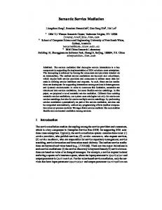
Figure 1. The basic mediated model and seven models that combine moderation and mediation. Panel A shows the basic mediated model. Panel B adds Z as a moderator of the path from X to M, which is the first stage of the mediated effect of X on Y. Panel C uses Z as a moderator of the path from M to Y, which is the second stage of the mediated effect of X on Y. Panel D integrates Panels B and C by specifying Z as a moderator of the first and second stages of the mediated effect. Panel E treats Z as a moderator of the path from X to Y, which is the direct effect of X on Y. Panels F and G add Z as a moderator of the first and second stages, respectively, of the mediated effect of X on Y. Panel H combines moderation of the direct effect with moderation of the first and second stages of the mediated effect, thereby moderating each path of the total effect of X on Y. For each panel, paths are labeled with coefficients from the regression equations used to estimate the model. For simplicity, the panels omit paths that lead directly from Z to M, to Y, or to both (these paths are implied by the regression equations for each model, where Z itself appears in each equation where it is used as a moderator variable).

MODERATION AND MEDIATION

the moderator variable refers to experimental conditions or naturally occurring subgroups, such as men and women, whereas in other cases a continuous moderator variable is dichotomized to form subgroups. Within each subgroup, mediation is usually assessed with the causal steps procedure, as summarized above (Baron & Kenny, 1986), or, in some instances, by testing the two paths that constitute the mediated effect and inferring support for mediation if both paths are significant (MacKinnon et al., 2002). If evidence for mediation differs between the subgroups, it is concluded that mediation is moderated by the subgrouping variable. The subgroup approach has been recommended in methodological discussions of moderation within the context of mediation (Wegener & Fabrigar, 2000) and structural equation modeling (Rigdon, Schumaker, & Wothke, 1998). The subgroup approach has several drawbacks. First, under standard assumptions, analyses conducted within each subgroup have lower statistical power than would be available from the full sample (J. Cohen, 1988). This reduction in statistical power has implications for tests of mediation in each subgroup. For instance, when the causal steps procedure is applied, low statistical power decreases the likelihood that the first three conditions will be satisfied and, conversely, increases the likelihood that the fourth condition will erroneously indicate complete mediation, which is evidenced by a nonsignificant relationship between X and Y when M is controlled. Given the generally modest levels of statistical power in psychology research (Maxwell, 2004; Rossi, 1990), procedures that sacrifice power should be avoided. Second, as noted earlier, studies that use the subgroup approach often form subgroups by dichotomizing a continuous moderator variable. This practice discards information, often yields biased parameter estimates, and further reduces statistical power (Maxwell & Delaney, 1993; Stone-Romero & Anderson, 1994). Although the dichotomization of continuous variables has been criticized for decades (J. Cohen, 1983; MacCallum, Zhang, Preacher, & Rucker, 2002; Maxwell & Delaney, 1993), this practice continues in psychology research and is common among studies that use the subgroup approach. Third, the subgroup approach does not provide tests of differences in mediation across levels of the moderator variable. Typically, studies that use the subgroup approach conclude that mediation is moderated when the conditions for mediation are satisfied in one subgroup but not in the other. Examining whether mediation is supported in either subgroup does not indicate whether mediation differs between the subgroups. Recall that, for the model in Figure 1A, the mediated effect of X on Y through M is represented by the product aX3bM4. Hence, moderated mediation would be reflected by differences in this product between subgroups, not by whether this product differs from zero in either subgroup. Studies that use the subgroup approach

5

sometimes test differences in individual paths between subgroups but rarely test the difference in the product that represents the mediated effect. Finally, studies that apply the subgroup approach usually assess mediation with the causal steps procedure (Baron & Kenny, 1986) and therefore suffer from its limitations (Collins et al., 1998; MacKinnon et al., 2002; Shrout & Bolger, 2002). Some studies that apply the subgroup approach analyze mediation within each subgroup by testing the product of the paths that constitute the mediated effect, but these studies are the exception rather than the rule.

Moderated Causal Steps Approach A third approach combines moderation and mediation by adding product terms to the regression equations involved in the causal steps procedure (Baron & Kenny, 1986; Muller, Judd, & Yzerbyt, 2005). Studies that apply this approach typically begin by using regression analysis to establish that Z moderates the relationship between X and Y, corresponding to Equation 1. At the second step, most studies examine whether Z moderates the effect of X on M, as captured by the following regression equation: M ⫽ a05 ⫹ aX5 X ⫹ aZ5 Z ⫹ aXZ5 XZ ⫹ eM5 .

(5)

The coefficient on XZ (i.e., aXZ5) indicates the extent to which the relationship between X and M varies across levels of Z. In the final step, most studies add M to Equation 1, yielding the following equation: Y ⫽ b06 ⫹ bX6 X ⫹ bZ6 Z ⫹ bXZ6 XZ ⫹ bM6 M ⫹ eY6 .

(6)

This equation is used to establish that M is related to Y, as evidenced by bM6, and to assess whether the XZ interaction captured by bXZ6 is no longer significant, which is taken as evidence that M mediates the effect of the XZ interaction on Y. Some studies modify this procedure either by testing whether the coefficient on X (i.e., bX6) rather than that on XZ remains significant or by testing the coefficients on X, Z, and XZ as a set. Other studies use alternative versions of Equation 6 that replace XZ with MZ or that contain both XZ and MZ (Muller et al., 2005). The moderated causal steps approach suffers from a number of shortcomings. Some of these shortcomings parallel those associated with the basic causal steps procedure. For instance, a nonsignificant interaction between X and Z in Equation 1 does not rule out the possibility that Z exerts moderating effects of opposite sign on the direct and indirect effects relating X to Y. In addition, the moderated causal steps approach does not directly estimate the extent to which Z influences the indirect effect of X on Y transmitted through M. Most studies examine the moderating effect of Z on the relationship between X and M, as indicated by aXZ5 in Equation 5; but studies rarely examine the moderating effect

6

EDWARDS AND LAMBERT

of Z on the relationship between M and Y or consider how the product representing the indirect effect of X on Y varies across levels of Z. Other shortcomings of the moderated causal steps approach go beyond those of the causal steps procedure itself. In particular, most studies that use the moderated causal steps approach examine moderation for only a subset of the paths linking X to Y. Support for moderation of one path can change when terms representing moderation for other paths are estimated. For instance, adding MZ to Equation 6 to estimate the moderating effect of Z on the path from M to Y will generally change the coefficient on XZ, which in turn can lead to different conclusions regarding the extent to which M mediates the moderating effect of Z on the relationship between X and Y. Moreover, hypothesizing that Z moderates a subset of the paths relating X to Y implies that the other paths are not moderated. Unless moderation is tested for each path, hypotheses concerning the moderating effects of Z are shielded from potentially disconfirming evidence. Another problem with the moderated causal steps approach is that testing whether the coefficient on XZ remains significant when M is controlled does not reveal how M influences the form of the interaction between X and Z, which is described by the coefficients on X, Z, and XZ as a set (Aiken & West, 1991). For example, assume that the coefficient estimates from Equation 1 indicate an ordinal interaction in which a positive relationship between X and Y becomes stronger as Z increases. If controlling for M renders the coefficient on XZ nonsignificant, then it follows that the relationship between X and Y no longer varies as a function of Z; however, it remains unclear whether the relationship is positive, negative, or null. These distinctions have substantive implications that are disregarded by focusing solely on the coefficient on XZ. A final problem is that studies that use the moderated causal steps approach rarely report coefficients relating X, M, and Y at specific levels of Z. These coefficients can be derived by using principles for computing simple slopes (Aiken & West, 1991) and are essential to interpreting the nature of the moderating effects of Z on the paths linking X, M, and Y. These paths can also be used to assess the magnitudes of the indirect effect and direct effect at different levels of Z to determine which effect dominates the total effect and how the relative contributions of the direct effect and indirect effect depend on Z. This evidence is essential to substantive interpretation but is generally disregarded by studies that use the moderated causal steps approach.

A General Path Analytic Framework for Combining Mediation and Moderation The general framework presented here builds on current approaches to combining moderation and mediation while

avoiding their attendant problems. This framework draws from methodological work that addresses moderation in the context of mediation, path analysis, and structural equation models (Baron & Kenny, 1986; James & Brett, 1984; Stolzenberg, 1980; Tate, 1998). In particular, we frame mediation in terms of a path model, express relationships among variables in the model by using regression equations, and incorporate moderation by supplementing these equations with the moderator variable and its product with the independent variable and the mediator variable (Baron & Kenny, 1986; James & Brett, 1984). We show how these equations can be integrated to represent moderation of the direct, indirect, and total effects of the model (Stolzenberg, 1980; Tate, 1998). This integration relies on reduced form equations (Johnston, 1984), which are derived by substituting the regression equation for the mediator variable into the equation for the dependent variable. We demonstrate how these reduced form equations can be used to express direct, indirect, and total effects at selected levels of the moderator variable (Tate, 1998). Our framework extends prior work on moderation and mediation in several key respects. First, the framework incorporates each of the logical possibilities that result when a moderator variable influences one or more of the paths of the basic mediated model in Figure 1A. Prior discussions of moderation and mediation have addressed only a subset of these possibilities. Second, we show that combining moderation and mediation does not yield a single path model but instead produces a set of models that each portray direct, indirect, and total effects at a particular level of the moderator variable. This perspective emphasizes that evidence for mediation varies according to the level of the moderator variable under consideration. Third, we point out that models that specify moderation of both paths of an indirect effect implicitly introduce a nonlinear effect for the moderating variable. This point has not been mentioned in discussions of such models (Baron & Kenny, 1986; James & Brett, 1984; Muller et al., 2005), yet it has important implications for conceptualizing and interpreting moderation of indirect effects. Finally, we demonstrate how to derive confidence intervals and conduct significance tests for direct, indirect, and total effects at selected levels of the moderator variable. These procedures have been discussed for mediated models that exclude moderation (MacKinnon et al., 2002; Shrout & Bolger, 2002; Sobel, 1982) but have not been addressed for models that combine moderation and mediation. The general framework presented here subsumes both moderated mediation and mediated moderation. As noted earlier, moderated mediation refers to a mediated effect that varies across levels of a moderator variable. In path analytic terms, moderated mediation means that either or both of the paths from X to M and from M to Y, which constitute the indirect effect of X on Y, vary across levels of the moderator

MODERATION AND MEDIATION

variable Z. Our framework accommodates moderation of these paths and therefore applies directly to moderated mediation. Mediated moderation means that an interaction between an independent and moderator variable affects a mediator variable that in turn affects an outcome variable. The interaction between the independent and moderator variables signifies that the effect of the independent variable on the mediator variable depends on the level of the moderator variable. Hence, in path analytic terms, mediated moderation indicates that the path from X to M varies across levels of Z, whereas the path from M to Y is unaffected by Z. Viewing moderated mediation and mediated moderation in terms of path analysis reveals that, when moderated mediation refers to moderation of the path from X to M but not of the path from M to Y, moderated mediation and mediated moderation are equivalent from an analytical standpoint, and any distinction between them is a matter of conceptual framing. When moderated mediation involves moderation of the path from M to Y, moderated mediation and mediated moderation are not analytically equivalent. The partial overlap between moderated mediation and mediated moderation adds to the confusion surrounding these terms (Muller et al., 2005). This confusion can be avoided by combining moderation and mediation by using the general path analytic framework developed here. With this framework, whether results are interpreted in terms of moderated mediation, mediated moderation, or neither depends on the conceptual orientation and tastes of the researcher. Because the framework we present relies on ordinary least squares (OLS) regression and path analysis, the statistical assumptions underlying these procedures merit attention (Berry, 1993; Bohrnstedt & Carter, 1971; J. Cohen, Cohen, West, & Aiken, 2003; Kenny, 1979; Pedhazur, 1997). These assumptions are summarized as follows: (a) Variables are measured without error; (b) measures are at the interval level; (c) residuals are normally distributed with zero mean and constant variance; (d) residuals are uncorrelated with one another and with the predictor variables in the equation in which each residual appears; (e) relationships among variables are unidirectional, thereby ruling out reciprocal relationships and feedback loops; (f) relationships among variables are additive and linear. Our framework adopts the first five assumptions, and we later discuss how the framework can be adapted when these assumptions are violated. The additivity assumption, which states that the dependent variable is an additive function of the predictor variables, is violated when predictor variables interact (J. Cohen et al., 2003). This violation is addressed by introducing product terms into the regression equation, as in Equation 1. Regression equations with product terms are nonadditive with respect to variables but are additive with respect to parameters (Berry, 1993; Neter, Wasserman, & Kutner, 1989) and therefore can be estimated with OLS regression. The regression equations that constitute our framework involve linear relationships, thereby incorporating the linearity as-

7

sumption, and we later discuss how the framework can be modified to accommodate nonlinear relationships. Finally, a fundamental assumption underlying our framework is that the causal relationships among variables are correctly specified. If an important relationship is omitted or the functional form of a relationship is not properly represented, the estimates produced by our framework can be biased. Like any application of regression analysis or path analysis, our framework does not itself generate evidence that establishes causality. Rather, it yields estimates of relationships among variables under the assumption that the causal structure of these relationships is correctly specified (Bohrnstedt & Carter, 1971; Duncan, 1975; Heise, 1969). This assumption is based on theory and research design and must be made prior to data analysis, given that the causal structure of a model dictates the equations and parameters that should be estimated (Duncan, 1975; Pedhazur, 1997). Conditions for establishing causality have been discussed extensively (Holland, 1986, 1988; Little & Rubin, 2000; Marini & Singer, 1988; Pearl, 2000; Rubin, 1974, 1978; Shadish, Cook, & Campbell, 2002; Sobel, 1996; West, Biesanz, & Pitts, 2000) and have implications for interpreting results from our framework. We return to these issues at the conclusion of this article.

Basic Mediated Model The point of departure for our general framework is the basic mediated model shown in Figure 1A. As noted earlier, this model depicts a direct effect of X on Y and an indirect effect of X on Y mediated by M. The direct and indirect effects of X on Y can be integrated into a single equation by substituting Equation 3 into Equation 4, which yields Y ⫽ b04 ⫹ bX4 X ⫹ bM4 共a03 ⫹ aX3 X ⫹ eM3 兲 ⫹ eY4 ⫽ b04 ⫹ bX4 X ⫹ a03 bM4 ⫹ aX3 bM4 X ⫹ bM4 eM3 ⫹ eY4 ⫽ b04 ⫹ a03 bM4 ⫹ 共bX4 ⫹ aX3 bM4 兲 X ⫹ eY4 ⫹ bM4 eM3 .

(7)

Equation 7 is a reduced form equation, which refers to an equation in which the terms on the right side are exclusively exogenous variables (Johnston, 1984). The compound coefficient for X is the sum of the direct effect bX4 and the indirect effect aX3bM4, which together capture the total effect of X on Y. Our framework builds on the basic mediated model by adding product terms involving Z to Equations 3 and 4 and deriving reduced form equations that show how Z influences the paths linking X, M, and Y and their associated indirect and total effects. We begin with models in which Z moderates either or both of the paths that constitute the indirect effect of X on Y transmitted through M. We highlight these models because they subsume both mediated moderation and moderated mediation. We then consider models in which Z also moderates the direct effect of X on Y, culminating with a model in which

EDWARDS AND LAMBERT

8

all three paths that form the indirect and direct effects of X on Y are moderated by Z.

equation for M is provided by Equation 3, whereas the regression equation for Y is as follows: Y ⫽ b010 ⫹ bX10 X ⫹ bM10 M ⫹ bZ10 Z

First Stage Moderation Model The initial moderated model we consider is shown in Figure 1B and incorporates Z as a moderator of the path from X to M.2 We call this first stage moderation because the moderating effect applies to the first stage of the indirect effect of X on Y. The regression equation for Y is provided by Equation 4, the same as that for the basic mediated model. The regression equation for M is given by Equation 5, which is typically used to evaluate the second condition of the moderated causal steps approach. Substituting Equation 5 into Equation 4 gives the reduced form equation for Y for the first stage moderation model: Y ⫽ b04 ⫹ bX4 X ⫹ bM4 共a05 ⫹ aX5 X ⫹ aZ5 Z ⫹ aXZ5 XZ ⫹ eM5 兲 ⫹ eY4 ⫽ b04 ⫹ bX4 X ⫹ a05 bM4 ⫹ aX5 bM4 X ⫹ aZ5 bM4 Z ⫹ aXZ5 bM4 XZ

⫽ b04 ⫹ a05 bM4 ⫹ 共bX4 ⫹ aX5 bM4 兲 X ⫹ aZ5 bM4 Z ⫹ aXZ5 bM4 XZ

(8)

Comparing Equation 8 with Equation 7 shows that the reduced form equation for the first stage moderation model adds Z and XZ as predictors of Y. The implications of these additional predictors can be seen by rewriting Equation 8 in terms of simple paths, which are analogous to simple slopes in moderated regression analysis (Aiken & West, 1991):

Y ⫽ b010 ⫹ bX10 X ⫹ bM10 共a03 ⫹ aX3 X ⫹ eM3 兲 ⫹ bZ10 Z ⫹ bMZ10 共a03 ⫹ aX3 X ⫹ eM3 兲 Z ⫹ eY10 ⫽ b010 ⫹ bX10 X ⫹ a03 bM10 ⫹ aX3 bM10 X ⫹ bM10 eM3 ⫹ bZ10 Z ⫹ a 03 bMZ10 Z ⫹ aX3 bMZ10 XZ ⫹ bMZ10 ZeM3 ⫹ eY10 ⫽ b010 ⫹ a03 bM10 ⫹ 共bX10 ⫹ aX3 bM10 兲 X ⫹ 共bZ10 ⫹ a03 bMZ10 兲 Z

(11)

Like the reduced form equation for the first stage moderation model (i.e., Equation 8), the reduced form equation for the second stage moderation model includes Z and XZ as predictors. However, the coefficients on these terms differ across the two equations. The implications of these differences can be seen by rewriting Equation 11 in terms of simple paths: Y ⫽ b010 ⫹ a03 bM10 ⫹ 共bZ10 ⫹ a03 bMZ10 兲 Z ⫹ 共bX10 ⫹ aX3 bM10 ⫹ aX3 bMZ10 Z兲 X ⫹ eY10 ⫹ bM10 eM3 ⫹ bMZ10 ZeM3

Y ⫽ b04 ⫹ a05 bM4 ⫹ aZ5 bM4 Z ⫹ 共bX4 ⫹ aX5 bM4 ⫹ aXZ5 bM4 Z兲 X

⫽ 关b010 ⫹ bZ10 Z ⫹ a03 共bM10 ⫹ bMZ10 Z兲兴

⫹ e Y4 ⫹ bM4 eM5

⫹ 关bX10 ⫹ aX3 共bM10 ⫹ bMZ10 Z兲兴 X

⫽ 关b04 ⫹ 共a05 ⫹ aZ5 Z兲bM4 兴 ⫹ 关bX4 ⫹ 共aX5 ⫹ aXZ5 Z兲bM4 兴 X ⫹ e Y4 ⫹ bM4 eM5 .

(10)

Equation 10 contains Z and MZ to represent the moderating effect of Z on the effect of M on Y. Substituting Equation 3 into Equation 10 yields the reduced form equation for Y associated with the second stage moderation model:

⫹ a X3 bMZ10 XZ ⫹ eY10 ⫹ bM10 eM3 ⫹ bMZ10 ZeM3 .

⫹ bM4 eM5 ⫹ eY4

⫹ eY4 ⫹ bM4 eM5 .

⫹ bMZ10 MZ ⫹ eY10 .

⫹ eY10 ⫹ bM10 eM3 ⫹ bMZ10 ZeM3 .

(12)

(9)

Whereas Equation 7 captures the indirect effect of X on Y as aX3bM4, Equation 9 represents the indirect effect with the compound term (aX5 ⫹ aXZ5Z)bM4. In this manner, Equation 9 shows that the path linking X to M, which is the first stage of the indirect effect of X on Y, varies as a function of Z. In contrast, the direct effect of X on Y, represented by bX4, is unaffected by Z. Equation 9 also shows that the intercept varies as a function of Z because of the contribution of aZ5Z. Selected values of Z can be substituted into Equation 9 to recover simple paths and effects that vary according to the level of Z. The use of these paths with the intercept from Equation 9 allows the simple paths and effects to be plotted to reveal the form of the moderating effect of Z.

Second Stage Moderation Model In the second stage moderation model, Z moderates the path from M to Y, as illustrated in Figure 1C. The regression

Comparing Equation 12 with Equation 9 shows that, whereas the first stage moderation model captures the indirect effect of X on Z as (aX5 ⫹ aXZ5Z)bM4, the second stage 2

In this article, we depict the moderating effects of Z as arrows from Z to the paths from X to M, M to Y, and X to Y. This approach to depicting moderation captures the notion that Z influences the magnitude of the relationship between the other variables in the model, which is consistent with how moderation is defined (Aiken & West, 1991). We should note, however, that moderation is symmetric, such that either of the variables involved in a two-way interaction can be cast as the moderator variable. For instance, if Z moderates the relationship between X and M, then it can also be said that X moderates the relationship between Z and M. Designating X or Z as the moderator variable is a matter of framing, and the relevant statistical procedures are the same regardless of whether X or Z is framed as the moderator variable. For the purposes of the framework developed here, we frame Z as the moderator variable.

MODERATION AND MEDIATION

moderation model depicts this effect as aX3(bM10 ⫹ bMZ10Z). As such, the portion of the indirect effect involving the path from M to Y varies as a function of Z. As before, the direct effect of X on Y (i.e., bX4 in Equation 9, bX10 in Equation 12) does not vary as a function of Z. The intercept of the reduced form equation is also affected by Z, as evidenced by the terms bZ10Z and bMZ10Z in Equation 12. By substituting values of Z into Equation 12, simple paths and effects can be derived and plotted to determine the form of the moderating effect of Z.

9

aXZ5bM4 for the first stage moderation model and aX3bMZ10 for the second stage moderation model. For these two models, the interaction effect does not vary according to the level of Z. The nature of the moderating effect of Z in the first and second stage moderation model is further clarified by rewriting Equation 14 in terms of simple paths, which yields the following: Y ⫽ 关b010 ⫹ a05 bM10 ⫹ 共bZ10 ⫹ aZ5 bM10 ⫹ a05 bMZ10 兲 Z ⫹ aZ5 bMZ10 Z 2 兴 ⫹ 关bX10 ⫹ aX5 bM10 ⫹ 共aXZ5 bM10 ⫹ aX5 bMZ10 兲 Z ⫹ aXZ5 bMZ10 Z 2 兴 X

⫹ eY10 ⫹ bM10 eM5 ⫹ bMZ10 ZeM5

First and Second Stage Moderation Model A model that combines first stage and second stage moderation is shown in Figure 1D. The regression equations for this model are Equation 5 for M and Equation 10 for Y. Substituting Equation 5 into Equation 10 yields the following reduced form equation: Y ⫽ b010 ⫹ bX10 X ⫹ bM10 共a05 ⫹ aX5 X ⫹ aZ5 Z ⫹ aXZ5 XZ ⫹ eM5 兲 ⫹ bZ10 Z ⫹ bMZ10 共a05 ⫹ aX5 X ⫹ aZ5 Z ⫹ aXZ5 XZ ⫹ eM5 兲 Z ⫹ eY10 ⫽ b010 ⫹ bX10 X ⫹ a05 bM10 ⫹ aX5 bM10 X ⫹ aZ5 bM10 Z ⫹ aXZ5 bM10 XZ ⫹ bM10 eM5 ⫹ bZ10 Z ⫹ a05 bMZ10 Z ⫹ aX5 bMZ10 XZ ⫹ aZ5 bMZ10 Z 2 ⫹ aXZ5 bMZ10 XZ 2 ⫹ bMZ10 ZeM5 ⫹ eY10 ⫽ b010 ⫹ a05bM10 ⫹ 共bX10 ⫹ aX5 bM10 兲 X ⫹ 共bZ10 ⫹ aZ5 bM10 ⫹ a05 bMZ10 兲 Z

⫹ aZ5 bMZ10 Z 2 ⫹ 共aXZ5 bM10 ⫹ aX5 bMZ10 兲 XZ ⫹ aXZ5 bMZ10 XZ 2 ⫹ eY10 ⫹ bM10 eM5 ⫹ bMZ10 ZeM5 .

(13)

Unlike the reduced form equations for the first stage moderation model and the second stage moderation model, the reduced form equation for the first and second stage moderation model includes Z 2 and XZ 2 as predictors. These additional terms indicate that the moderating effect of Z on the relationship between X and Y varies as a function of Z itself. This point is revealed by rewriting Equation 13 as follows:

⫹ 关bX10 ⫹ 共aX5 ⫹ aXZ5 Z兲共bM10 ⫹ bMZ10 Z兲兴 X ⫹ e Y10 ⫹ bM10 eM5 ⫹ bMZ10 ZeM5 .

(15)

Equation 15 shows that Z affects both of the paths that constitute the indirect effect of X on Y, which is represented by the compound term (aX5 ⫹ aXZ5Z)(bM10 ⫹ bMZ10Z). As with the previous two models, the direct effect of X on Y, which is represented by bX10, is unaffected by Z. The intercept of the reduced form equation is again influenced by Z, as shown by the terms bZ10Z, aZ5Z, and bMZ10Z in Equation 15. Substituting values of Z into Equation 15 produces simple paths and effects that show the form of the moderating effect associated with Z.

Direct Effect Moderation Model We now demonstrate how Z can be incorporated as a moderator of the direct effect of X on Z, laying the foundation for models that combine moderation of direct and indirect effects. Applying moderation to the direct effect of the basic mediated model yields the direct effect moderation model shown in Figure 1E. The regression equation for M is Equation 3, and the regression Equation for Y is Equation 6, which is typically used to assess the third and fourth conditions of the moderated causal steps approach. Substituting Equation 3 into Equation 6 gives the following reduced form equation: Y ⫽ b06 ⫹ bX6 X ⫹ bZ6 Z

Y ⫽ b010 ⫹ a05 bM10 ⫹ 共bX10 ⫹ aX5 bM10 兲 X

⫹ bXZ6 XZ ⫹ bM6 共a03 ⫹ aX3 X ⫹ eM3 兲 ⫹ eY6

⫹ 共bZ10 ⫹ aZ5 bM10 ⫹ a05 bMZ10 ⫹ aZ5 bMZ10 Z兲 Z

⫽ b06 ⫹ bX6 X ⫹ bZ6 Z ⫹ bXZ6 XZ

⫹ 共aXZ5 bM10 ⫹ aX5 bMZ10 ⫹ aXZ5 bMZ10 Z兲 XZ ⫹ e Y10 ⫹ bM10 eM5 ⫹ bMZ10 ZeM5 .

⫽ 关b010 ⫹ bZ10 Z ⫹ 共a05 ⫹ aZ5 Z兲共bM10 ⫹ bMZ10 Z兲兴

(14)

⫹ a03 bM6 ⫹ aX3 bM6 X ⫹ bM6 eM3 ⫹ eY6 ⫽ b06 ⫹ a03 bM6 ⫹ 共bX6 ⫹ aX3 bM6 兲 X

Equation 14 shows that the coefficient on the interaction term XZ is the compound expression (aXZ5bM10 ⫹ aX5bMZ10 ⫹ aXZ5bMZ10Z). Hence, the magnitude of the interaction effect is influenced by the level of Z, as indicated by the term aXZ5bMZ10Z. In contrast, the coefficient on XZ is

⫹ bZ6 Z ⫹ bXZ6 XZ ⫹ eY6 ⫹ bM6 eM3 .

(16)

In Equation 16, the coefficient on XZ is simply bXZ6, as opposed to the compound coefficients that result when Z moderates either or both stages of the indirect effect. Re-

EDWARDS AND LAMBERT

10

writing Equation 16 in terms of simple paths yields the following: Y ⫽ b06 ⫹ a03 bM6 ⫹ bZ6 Z ⫹ 共bX6 ⫹ aX3 bM6 ⫹ bXZ6 Z兲 X ⫹ e Y6 ⫹ bM6 eM3 ⫽ 关b06 ⫹ bZ6 Z ⫹ a03 bM6 兴 ⫹ 关共bX6 ⫹ bXZ6 Z兲 ⫹ aX3 bM6 兴 X ⫹ e Y6 ⫹ bM6 eM3 .

(17)

Equation 17 shows that the direct effect of X on Y, represented by (bX6 ⫹ bXZ6Z), varies across levels of Z, whereas the indirect effect captured by aX3bM6 does not depend on Z. Equation 17 also shows that the intercept is influenced by Z due to the term bZ6Z.

X on Y varies as a function of Z, as captured by the term (aX5 ⫹ aXZ5Z)bM6. However, Equation 19 shows that the direct effect of X on Y also depends on Z, due to the term (bX6 ⫹ bXZ6Z). The intercept in Equation 19 is also affected by Z, as reflected by the terms bZ6Z and aZ5Z.

Second Stage and Direct Effect Moderation Model Combing direct effect moderation with second stage moderation yields the second stage and direct effect moderation model in Figure 1G. For this model, the regression equation for M is Equation 3, and the regression equation for Y is the following: Y ⫽ b020 ⫹ bX20 X ⫹ bM20 M ⫹ bZ20 Z ⫹ bXZ20 XZ ⫹ bMZ20 MZ ⫹ eY20 .

First Stage and Direct Effect Moderation Model We now add direct effect moderation to models in which the indirect effect is moderated. We start by adding direct effect moderation to the first stage moderation model, yielding the first stage and direct effect moderation model in Figure 1F. For this model, the equations for M and Y are Equation 5 and Equation 6, respectively. Substituting Equation 5 into Equation 6 produces the following reduced form equation: Y ⫽ b06 ⫹ bX6 X ⫹ bZ6 Z ⫹ bXZ6 XZ

Equation 20 contains both XZ and MZ, thereby capturing the moderating effects of Z on the relationships of X and M with Y. Substituting Equation 3 into Equation 20 gives the reduced form equation: Y ⫽ b020 ⫹ bX20 X ⫹ bM20 共a03 ⫹ aX3 X ⫹ eM3 兲 ⫹ bZ20 Z ⫹ bXZ20 XZ ⫹ bMZ20 共a03 ⫹ aX3 X ⫹ eM3 兲 Z ⫹ eY20 ⫽ b020 ⫹ bX20 X ⫹ a03 bM20 ⫹ aX3 bM20 X ⫹ bM20 eM3 ⫹ bZ20 Z ⫹ bXZ20 XZ ⫹ a03 bM20 Z ⫹ aX3 bMZ20 XZ ⫹ bMZ20 ZeM3 ⫹ eY20

⫹ bM6 共a05 ⫹ aX5 X ⫹ aZ5 Z ⫹ aXZ5 XZ ⫹ eM5 兲 ⫹ eY6

⫽ b020 ⫹ a03 bM20 ⫹ 共bX20 ⫹ aX3 bM20 兲 X ⫹ 共bZ20 ⫹ a03 bMZ20 兲 Z ⫹ (bXZ20 ⫹ aX3 bMZ20 ) XZ ⫹ eY20 ⫹ bM20 eM3 ⫹ bMZ20 ZeM3 .

⫽ b06 ⫹ bX6 X ⫹ bZ6 Z ⫹ bXZ6 XZ

(21)

⫹ a05 bM6 ⫹ aX5 bM6 X ⫹ aZ5 bM6 Z ⫹ aXZ5 bM6 XZ ⫹ eY6 ⫹ bM6 eM5

As before, the moderating effect of Z is highlighted by rewriting Equation 21 in terms of simple paths:

⫽ b06 ⫹ a05 bM6 ⫹ 共bX6 ⫹ aX5 bM6 兲 X ⫹ 共bZ6 ⫹ aZ5 bM6 兲 Z ⫹ 共bXZ6 ⫹ aXZ5 bM6 兲 XZ ⫹ eY6 ⫹ bM6 eM5 .

(20)

(18)

As with the previous models, the moderating effect of Z for the first stage and direct effect moderation model can be clarified by rewriting Equation 18 in terms of simple paths: Y ⫽ b06 ⫹ a05 bM6 ⫹ 共bZ6 ⫹ aZ5 bM6 兲 Z

Y ⫽ b020 ⫹ a03 bM20 ⫹ 共bZ20 ⫹ a03 bMZ20 兲 Z ⫹ 关共bX20 ⫹ aX3 bM20 兲 ⫹ 共bXZ20 ⫹ aX3 bMZ20 兲 Z兴 X ⫹ eY20 ⫹ bM20 eM3 ⫹ bMZ20 ZeM3 ⫽ 关b020 ⫹ bZ20 Z ⫹ a03 共bM20 ⫹ bMZ20 Z兲兴 ⫹ 关共bX20 ⫹ bXZ20 Z兲 ⫹ aX3 共bM20 ⫹ bMZ20 Z兲兴 X

⫹ 关共bX6 ⫹ aX5 bM6 兲 ⫹ 共bXZ6 ⫹ aXZ5 bM6 兲 Z兴 X

⫹ eY20 ⫹ bM20 eM3 ⫹ bMZ20 ZeM3 .

(22)

⫹ eY6 ⫹ bM6 eM5 Y ⫽ 关b06 ⫹ bZ6 Z ⫹ 共a05 ⫹ aZ5 Z兲bM6 兴 ⫹ 关共bX6 ⫹ bXZ6 Z兲 ⫹ 共aX5 ⫹ aXZ5 Z兲bM6 兴 X ⫹ eY6 ⫹ bM6 eM5 .

(19)

Like Equation 9 for the first stage moderation model, Equation 19 indicates that the first stage of the indirect effect of

As with Equation 12 for the second stage moderation model, Equation 22 shows that the second stage of the indirect effect of X on Y depends on Z, as indicated by the term aX3(bM20 ⫹ bMZ20Z). However, Equation 22 adds moderation of the direct effect of X on Y, as captured by the term (bX20 ⫹ bXZ20Z). The intercept in Equation 22 also varies across levels of Z because of the terms bZ20Z and bMZ20Z.

MODERATION AND MEDIATION

Total Effect Moderation Model Finally, the model in Figure 1H combines moderation of the first and second stages of the indirect effect with moderation of the direct effect. We call this model the total effect moderation model, given that a total effect represents the combination of direct and indirect effects (Alwin & Hauser, 1975). For the total effect moderation model, the regression equation for M is provided by Equation 5, and the regression equation for Y is Equation 20. Substituting Equation 5 into Equation 20 gives the reduced form equation for the total effect moderation model:

11

tute the indirect effect of X on Y, as indicated by the term (aX5 ⫹ aXZ5Z)(bM20 ⫹ bMZ20Z), as well as the path representing the direct effect of X on Y, which corresponds to the term (bX20 ⫹ bXZ20Z). The reduced form equation also shows that Z affects the intercept through bZ20Z, aZ5Z, and bMZ20Z. Hence, substituting values of Z into Equation 25 yields simple paths and effects that can be analyzed and plotted to determine the form of the moderating effect of Z on the direct, indirect, and total effects of X on Y, as we later demonstrate.

Model Estimation and Interpretation Y ⫽ b020 ⫹ bX20 X ⫹ bM20 共a05 ⫹ aX5 X ⫹ aZ5 Z ⫹ aXZ5 ZX ⫹ eM5 兲 ⫹ bZ20 Z ⫹ bXZ20 XZ ⫹ bMZ20 共a05 ⫹ aX5 X ⫹ aZ5 Z ⫹ aXZ5 XZ ⫹ eM5 兲 Z ⫹ eY20 ⫽ b020 ⫹ bX20 X ⫹ a05 bM20 ⫹ aX5 bM20 X ⫹ aZ5 bM20 Z ⫹ aXZ5 bM20 XZ ⫹ bM20 eM5 ⫹ bZ20 Z ⫹ bXZ20 XZ ⫹ a05 bMZ20 Z ⫹ aX5 bMZ20 XZ ⫹ aZ5 bMZ20 Z 2 ⫹ aXZ5 bMZ20 XZ 2 ⫹ bMZ20 ZeM5 ⫹ eY20 ⫽ b020 ⫹ a05 bM20 ⫹ 共bX20 ⫹ aX5 bM20 兲 X ⫹ 共bZ20 ⫹ aZ5 bM20 ⫹ a05 bMZ20 兲 Z ⫹ aZ5 bMZ20 Z 2 ⫹ 共bXZ20 ⫹ aXZ5 bM20 ⫹ aX5 bMZ20 兲 XZ ⫹ aXZ5 bMZ20 XZ 2 ⫹ eY20 ⫹ bM20 eM5 ⫹ bMZ20 ZeM5 .

(23)

Like the reduced form equation for the first and second stage moderation model, the reduced form equation for the total effect moderation model contains Z 2 and XZ 2, such that the moderating effect of Z on the relationship between X and Y depends on the level of Z. This can be seen by expressing Equation 23 in a form similar to Equation 14: Y ⫽ b020 ⫹ a05 bM20 ⫹ 共bX20 ⫹ aX5 bM20 兲 X ⫹ 共bZ20 ⫹ aZ5 bM20 ⫹ a05 bMZ20 ⫹ aZ5 bMZ20 Z兲 Z ⫹ 共bXZ20 ⫹ aXZ5 bM20 ⫹ aX5 bMZ20 ⫹ aXZ5 bMZ20 Z兲 XZ ⫹ e Y20 ⫹ bM20 eM5 ⫹ bMZ20 ZeM5 .

(24)

Like Equation 14, Equation 24 shows that the coefficient on the interaction term XZ depends on the level of Z, as reflected by the term aXZ5bMZ20Z. The moderating effects of Z embodied by the total effect moderation model can be seen by rewriting Equation 24 in terms of simple paths, as follows: Y ⫽ 关b020 ⫹ a05 bM20 ⫹ 共bZ20 ⫹ aZ5 bM20 ⫹ a05 bMZ20 兲 Z ⫹ aZ5 bMZ20 Z 2 兴 ⫹ 关bX20 ⫹ aX5 bM20 ⫹ 共bXZ20 ⫹ aXZ5 bM20 ⫹ aX5 bMZ20 兲 Z ⫹ aXZ5 bMZ20 Z 2 兴 X ⫹ eY20 ⫹ bM20 eM5 ⫹ bMZ20 ZeM5 ⫽ 关b020 ⫹ bZ20 Z ⫹ 共a05 ⫹ aZ5 Z兲共bM20 ⫹ bMZ20 Z兲兴 ⫹ 关共bX20 ⫹ bXZ20 Z兲 ⫹ 共aX5 ⫹ aXZ5 Z兲共bM20 ⫹ bMZ20 Z兲兴 X ⫹ eY20 ⫹ bM20 eM5 ⫹ bMZ20 ZeM5 .

(25)

Equation 25 shows that Z affects the two paths that consti-

The equations for the models summarized above can be estimated with OLS regression, and coefficients from the equations can be tested with conventional procedures (J. Cohen et al., 2003; Pedhazur, 1997). However, the reduced form equations contain products of regression coefficients, which must be tested with procedures that take into account sampling distributions of products of random variables. One procedure is based on methods for deriving the variance of the product of two random variables (Bohrnstedt & Goldberger, 1969; Goodman, 1960), of which the Sobel (1982) approach is perhaps the best known (MacKinnon et al., 2002). With this procedure, the product of two regression coefficients is divided by the square root of its estimated variance, and the resulting ratio is interpreted as a t statistic. Although this procedure is useful, it relies on the assumption that the sampling distribution of the product of two random variables is normal, given that the procedure uses only the variance to represent the distribution of the product. This assumption is tenuous because the distribution of a product is nonnormal, even when the variables constituting the product are normally distributed (Anderson, 1984). The foregoing assumption can be relaxed with the bootstrap (Efron & Tibshirani, 1993; Mooney & Duval, 1993; Stine, 1989). The bootstrap generates a sampling distribution of the product of two regression coefficients by repeatedly estimating the coefficients with bootstrap samples, each of which contains N cases randomly sampled with replacement from the original sample, in which N is the size of the original sample. Coefficient estimates from each bootstrap sample are used to compute the product, and these products are rank ordered to locate percentile values that bound the desired confidence interval (e.g., the 2.5 and 97.5 percentiles for a 95% confidence interval). Confidence intervals constructed in this manner should be adjusted for any difference between the product from the full sample and the median of the products estimated from the bootstrap samples, yielding a bias-corrected confidence interval (Efron & Tibshirani, 1993; Mooney & Duval, 1993; Stine, 1989). When constructing confidence intervals, a minimum of 1,000 bootstrap samples should be used to accurately

EDWARDS AND LAMBERT

12

locate the upper and lower bounds of the 95% confidence interval (Efron & Tibshirani, 1993; Mooney & Duval, 1993). The bootstrap has been used to test indirect effects in mediated models (MacKinnon, Lockwood, & Williams, 2004; Shrout & Bolger, 2002) and can be extended to models that combine mediation and moderation, as we later illustrate. As noted earlier, simple effects can be computed by substituting selected values of Z into the reduced form equations. When Z is a continuous variable, we recommend the use of values that are substantively or practically meaningful (e.g., a clinical cutpoint). If such values cannot be identified, we suggest the use of representative scores in the distribution of Z, such as one standard deviation above and below its mean (Aiken & West, 1991). When Z is a categorical variable, scores used to code Z should be used to obtain simple effects for each category. Simple effects represented by single paths can be tested with procedures for simple slopes (Aiken & West, 1991), and simple effects that involve products of paths, such as simple indirect and total effects, can be tested with confidence intervals derived from the bootstrap. The form of the moderating effects of Z can be further clarified by plotting simple paths and simple effects for the selected values of Z.

Empirical Example Sample and Measures The following example uses data from 1,307 respondents who were surveyed on work and family issues (Edwards & Rothbard, 1999; Kossek, Colquitt, & Noe, 2001). Of the respondents (age: M ⫽ 39 years), most were women (66%), Caucasian (86%), married (66%), and had completed an undergraduate program (66%). Respondents held various jobs ranging from clerical and blue collar positions to professional, medical, administrative, and faculty positions. We examine a mediated model in which feedback from family members is posited to influence commitment to family both directly and indirectly through satisfaction with family. These effects are moderated by either gender or family centrality to demonstrate the use of categorical and continuous moderator variables, respectively. Feedback was measured with five items that described reactions to performance of the family role (e.g., My family thinks what I do at home is outstanding). Satisfaction with family was measured with three items that described positive feelings toward the family (e.g., In general, I am satisfied with my family life). Commitment was measured with eight items that described psychological attachment to the family (e.g., I feel a great sense of commitment to my family). Family centrality was assessed with six items that described the importance of family to life as a whole (e.g., The most

important things that happen in life involve family). All items used 7-point response scales in which higher scores represented greater endorsement of the item (1 ⫽ strongly disagree, 7 ⫽ strongly agree). Prior to analysis, all continuous measures were mean centered, whereas gender was coded 0 for men and 1 for women (Aiken & West, 1991).3

Analyses For illustration, we analyzed the total effect moderation model, the most general of the eight models shown in Figure 1. This model is represented by Equations 5 and 20, which were estimated using SPSS (Version 14.0; 2005, SPSS Inc.). The regression module was used to estimate coefficients for the full sample, and the constrained nonlinear regression (CNLR) module was used to estimate coefficients from 1,000 bootstrap samples. Unlike the regression module, the CNLR module contains an algorithm that draws bootstrap samples, estimates regression coefficients for each sample, and writes the coefficients to an output file. We used the default loss function of the CNLR module, which minimizes the sum of squared residuals, thereby producing OLS coefficient estimates. Individual coefficients from Equations 5 and 20 were tested using the standard errors reported by the regression module. Expressions that contained products of coefficients, such as indirect and total effects, were tested with biascorrected confidence intervals based on the bootstrap coefficient estimates generated by the CNLR module. These confidence intervals were constructed by opening the SPSS output files, resaving them as Microsoft Excel files, and opening these files with Excel 2003. Using Equation 25, formulas were written into the Excel file to compute simple paths, indirect effects, and total effects at selected levels of the moderator variables (0 and 1 for gender, one standard deviation above and below the mean for centrality). These formulas were applied to coefficient estimates from each bootstrap sample, producing 1,000 estimates of each simple path, indirect effect, and total effect. Additional formulas 3

As an alternative to dummy coding, researchers could use effect coding or contrast coding when independent or moderator variables are nominal or ordinal. For instance, if a moderator variable represents two experimental groups of equal size, then assigning effect codes of ⫺0.5 and 0.5 to Z will produce coefficients on X and M that represent average effects of these variables. Simple paths could be recovered by substituting ⫺0.5 and 0.5 into the equations for the model being tested. This and other coding options for nominal and ordinal variables are discussed by West, Aiken, and Krull (1996). Regardless of the coding method used, it should be emphasized that, when a regression equation contains product terms, the coefficients on the variables that constitute the product represent conditional effects, such that the coefficient on each variable represents the effect of that variable when the other variable in the product equals zero (Aiken & West, 1991).

MODERATION AND MEDIATION

were used to compute differences between each path and effect across levels of the moderator variable, which were also applied to the 1,000 bootstrap estimates. The Excel percentile function was used to locate the 2.5 and 97.5 percentiles of the paths and effects computed from the bootstrap estimates, establishing the bounds of the 95% confidence interval. These bounds were adjusted with formulas reported by Stine (1989, p. 277), which were also written into the Excel file, to obtain bias-corrected confidence intervals. These confidence intervals were used to test indirect effects, total effects, and differences in these effects across levels of the moderator variables such that, if the 95% confidence interval excluded 0, the quantity being tested was declared statistically significant. A sample of the SPSS regression and CNLR syntax used to produce regression and bootstrap estimates is provided in the Appendix, and all SPSS and Excel files are available online at http//:dx.doi.org/10.1037/1082989X.12.1.1.supp Regression results are reported in Table 1, and simple effects are given in Table 2, including effects that represent the three paths of the basic mediated model as well as the indirect and total effects of the model. Models depicting simple paths are shown in Figure 2, and plots of simple effects are given in Figure 3 and Figure 4. Plots of the first stage of the indirect effect used (a05 ⫹ aZ5Z) as the intercept and (aX5 ⫹ aXZ5Z) as the slope (Aiken & West, 1991). For the second stage, the intercept and slope were derived by rewriting Equation 20 as follows: Y ⫽ 关b020 ⫹ bZ20 Z ⫹ 共bX20 ⫹ bXZ20 Z兲 X兴 ⫹ 共bM20 ⫹ bMZ20 Z兲 M ⫹ eY20 .

(26)

Equation 26 shows that the slope relating M to Y is (bM20 ⫹ bMZ20Z), which matches the second stage of the indirect effect in Equation 25. Equation 26 also indicates that the intercept of the function relating M to Y, represented by the compound term [b020 ⫹ bZ20Z ⫹ (bX20 ⫹ bXZ20Z)X], depends on the level of X. For plotting purposes, we suggest the use of the mean of X to compute the intercept. When X

13

Table 2 Analysis of Simple Effects Moderator variable Gender Men Women Differences Centrality Low High Differences

Stage

Effect

First

Second

Direct

Indirect

Total

0.81** 0.67** 0.14**

0.31** 0.30** 0.01

0.28** 0.15** 0.13**

0.25** 0.20** 0.05

0.53** 0.35** 0.18**

0.70** 0.60** 0.10*

0.30** 0.14** 0.16**

0.17** 0.07** 0.10**

0.21** 0.08** 0.13**

0.38** 0.15** 0.23**

Note. N ⫽ 1,307. For rows labeled men, women, low, and high, table entries are simple effects computed from Equation 25 using coefficient estimates from Table 1. Zs ⫽ 0 and 1 for men and women, respectively; Z ⫽ ⫺0.91 and 0.91 for low and high centrality, respectively (i.e., one standard deviation above and below the mean of the centered centrality variable). For gender, differences in simple effects were computed by subtracting the effects for women from the effects for men. For centrality, differences in simple effects were computed by subtracting the effects for high centrality from the effects for low centrality. Tests of differences for the first stage, second stage, and direct effect are equivalent to tests of aXZ5, bMZ20, and bXZ20, respectively, as reported in Table 1. Tests of differences for the indirect and total effect were based on bias-corrected confidence intervals derived from bootstrap estimates. * p ⬍ .05. ** p ⬍ .01.

is mean-centered, as in the present illustration, the mean of X equals 0, and the intercept simplifies to (b020 ⫹ bZ20Z). Plots for the direct, indirect, and total effects were based on Equation 25, which expresses the direct effect as (bX20 ⫹ bXZ20Z), the indirect effect as (aX5 ⫹ aXZ5Z)(bM20 ⫹ bMZ20Z), and the total effect as [(bX20 ⫹ bXZ20Z) ⫹ (aX5 ⫹ aXZ5Z)(bM20 ⫹ bMZ20Z)]. These expressions were used as the slopes for each effect. All three effects shared the common intercept of [b020 ⫹ bZ20Z ⫹ (a05 ⫹ aZ5Z)(bM20 ⫹ bMZ20Z)], which equals the expected value of Y when X equals 0 for each effect. For display purposes, the axes for each figure were converted back to their original (i.e., uncentered) scales, which facilitates interpretation but does not alter the form of the plotted interaction (Aiken & West, 1991, p. 15).

Table 1 Coefficient Estimates Moderator variable

aX5

aZ5

aXZ5

R2

bX20

bM20

bZ20

bXZ20

bMZ20

R2

Gender Centrality

0.81** 0.65**

⫺0.05 0.17**

⫺0.14** ⫺0.05*

0.45** 0.46**

0.28** 0.12**

0.31** 0.22**

0.06 0.33**

⫺0.13** ⫺0.05**

⫺0.01 ⫺0.09**

0.42** 0.57**

Note. N ⫽ 1,307. Entries under columns labeled aX5, aZ5, and aXZ5 are unstandardized coefficient estimates from Equation 5, which uses satisfaction as the dependent variable. Entries under columns labeled bX20, bM20, bZ20, bXZ20, and bMZ20 are unstandardized coefficient estimates from Equation 20, which uses commitment as the dependent variable. Coefficients in the first row are from equations that use gender as the moderator variable, and coefficients in the second row are from equations that use centrality as the moderator variable. * p ⬍ .05. ** p ⬍ .01.

EDWARDS AND LAMBERT

14

Figure 2. Mediated models showing simple effects for men and women and for low and high centrality. For each model, X represents feedback, M signifies satisfaction, and Y indicates commitment. Coefficients in boldface were significantly different (p ⬍ .05) across levels of the moderator variable (i.e., gender for Panels A and B, centrality for Panels C and D). Panels A and B show that gender moderated the paths from feedback to satisfaction and satisfaction to commitment, both of which were larger for men than for women. Panels C and D indicate that centrality moderated all three paths relating feedback, satisfaction, and commitment, which were larger when centrality was low than when it was high.

Results for Gender Moderation We first consider results for gender as the moderator variable. Coefficient estimates in Table 1 show that gender moderated the path from feedback to satisfaction (aXZ5 ⫽ ⫺0.14, p ⬍ .01), the path from feedback to commitment (bXZ20 ⫽ ⫺0.13, p ⬍ .01), but not the path from satisfaction to commitment (bMZ20 ⫽ ⫺0.01, p ⬎ .05). Equation 25 was applied to coefficients in Table 1 to compute simple effects, as reported in Table 2 and portrayed in Figures 2A and 2B. For men, Z ⫽ 0, and the first stage, second stage, and direct effect reduce to aX5, bM20, and bX20, respectively, which equal 0.81, 0.31, and 0.28. The indirect effect for men equals the product of the first and second stages, or 0.81 ⫻ 0.31 ⫽ 0.25, and the total effect equals the sum of the direct and indirect effects, or 0.28 ⫹ 0.25 ⫽ 0.53. For women, Z ⫽ 1, such that the first stage of the indirect effect becomes aX5 ⫹ aXZ5 ⫽ 0.81 ⫺ 0.14 ⫽ 0.67, the second stage becomes bM20 ⫹ bMZ20 ⫽ 0.31 ⫺ 0.01 ⫽ .030, and the direct effect becomes bX20 ⫹ bXZ20 ⫽ 0.28 ⫺ 0.13 ⫽ 0.15. As for men, the indirect effect for women equals the product of the first and second stages, or 0.67 ⫻ 0.30 ⫽ 0.20, and the total effect is the sum of the direct and indirect effects, or 0.15 ⫹ 0.20 ⫽ 0.35. Comparing these effects for men and women shows that the first stage of the indirect effect was stronger for men (0.81 ⫺ 0.67 ⫽ 0.14, p ⬍ .01), whereas the second stage did not differ for men and women (0.31 ⫺ 0.30 ⫽ 0.01, p ⬎ .05). When multiplied, the first and second stages did not produce a significant difference in the indirect effect for men and women (0.25 ⫺ 0.20 ⫽ 0.05, p ⬎ .05).

However, the direct effect was stronger for men than for women (0.28 ⫺ 0.15 ⫽ 0.13, p ⬍ .01) and, when combined with the indirect effect, produced a larger total effect for men (0.53 ⫺ 0.35 ⫽ 0.18, p ⬍ .01). Differences in these effects are depicted as simple slopes in Figures 3A through 3E. As seen by comparing Figures 3A and 3C, the moderating effect of gender on the first stage was not sufficient to produce a meaningful difference in slopes for the indirect effect because of the absence of a moderating effect of gender on the second stage indicated by Figure 3B. Comparing Figures 3C and 3D further shows that the difference in slopes for the direct effect was the primary reason for the difference in slopes for the total effect in Figure 3E. Thus, gender moderated the direct effect of feedback on commitment and the first stage of the indirect effect of feedback on commitment mediated by satisfaction, and these differences were sufficient to produce a larger total effect for men.

Results for Centrality Moderation For centrality as the moderator variable, coefficient estimates in Table 1 show that centrality moderated the path from feedback to satisfaction (aXZ5 ⫽ ⫺0.05, p ⬍ .05), the path from satisfaction to commitment (bMZ20 ⫽ ⫺0.09, p ⬍ .01), and the feedback to commitment (bXZ20 ⫽ ⫺0.05, p ⬍ .01). Coefficients in Table 1 were again used to compute simple effects, which are reported in Table 2 and depicted in Figures 2C and 2D. For low centrality (i.e., one standard (text continues on page 17)

Figure 3. Plots of simple paths and effects with gender as the moderator variable. In Panel A, the slope of the first stage of the mediated effect is steeper for men than for women. However, as seen in Panels B and C, the slopes of the second stage and indirect effect, respectively, do not differ for men and women. In contrast, Panel D depicts a steeper slope of the direct effect for men than for women. Finally, Panel E, which combines the simple slopes in Panels C and D, shows that the total effect was steeper for men than for women.

Figure 4. Plots of simple paths and effects with centrality as the moderator variable. In Panels A and B, the first and second stages, respectively, of the mediated effect had steeper slopes when centrality was low rather than when it was high. Correspondingly, the indirect effect depicted in Panel C was steeper for low centrality. The direct effect shown in Panel D was also steeper when centrality was low. Finally, as would be expected, the total effect in Panel E, which combines the indirect and direct effects, was steeper for low centrality than for high centrality.

MODERATION AND MEDIATION

deviation below the mean), Z ⫽ ⫺0.91, such that the first stage of the indirect effect (aX5 ⫹ aXZ5Z) equals 0.65 ⫺ 0.05(– 0.91) ⫽ 0.70. The second stage of the indirect effect (bM20 ⫹ bMZ20Z) equals 0.22 ⫺ 0.09(⫺0.91) ⫽ 0.30. Finally, the direct effect (bX20 ⫹ bXZ20Z) equals 0.12 ⫺ 0.05(⫺0.91) ⫽ 0.17. The indirect effect for low centrality equals the product of the first and the second stages, or 0.70 ⫻ 0.30 ⫽ 0.21, and the total effect equals the sum of the direct and indirect effects, or 0.17 ⫹ 0.21 ⫽ 0.38. For high centrality (i.e., one standard deviation above the mean), Z ⫽ 0.91, and the first stage of the indirect effect equals 0.65 ⫺ 0.05(0.91) ⫽ 0.60, the second stage equals 0.22 ⫺ 0.09(0.91) ⫽ 0.14, and the direct effect is 0.12 ⫺ 0.05(0.91) ⫽ 0.07. The indirect effect equals the product of the first and second stages, or 0.60 ⫻ 0.14 ⫽ 0.08, and the total effect is the sum of the direct and indirect effects, or 0.07 ⫹ 0.08 ⫽ 0.15. Differences in the effects for low and high centrality indicate that the first stage of the indirect effect was stronger for low centrality (0.70 ⫺ 0.60 ⫽ 0.10, p ⬍ .05) and, similarly, the second stage of the indirect effect was also stronger for low centrality (0.30 ⫺ 0.14 ⫽ 0.16, p ⬍ .01). These differences contributed to a significantly stronger indirect effect for low centrality (0.21 ⫺ 0.08 ⫽ 0.13, p ⬍ .01). The direct effect was also stronger for low centrality (0.17 ⫺ 0.07 ⫽ 0.10, p ⬍ .01) and, when added to the indirect effect, produced a stronger total effect for low centrality (0.38 ⫺ 0.15 ⫽ 0.23, p ⬍ .01).4 Figures 4A through 4E show differences in simple slopes for low and high centrality. Figure 4A shows that, for the first stage of the indirect effect, the relationship between feedback and satisfaction was steeper for respondents who reported low rather than high centrality, and high centrality respondents reported higher satisfaction across all levels of feedback. Similarly, as shown in Figure 4B, the relationship between satisfaction and commitment was steeper for low centrality respondents, and commitment was higher at all levels of satisfaction for high centrality respondents. This pattern held for the indirect, direct, and total effects in Figures 4C, 4D, and 4E, respectively, each of which indicated a steeper slope between feedback and commitment for low centrality respondents and a higher intercept for high centrality respondents. Hence, centrality moderated each path of the mediated model relating feedback, satisfaction, and commitment, such that the indirect and direct effects relating feedback to commitment were stronger when centrality was low, although commitment was higher at all levels of feedback when centrality was high.

Discussion This article presents a general framework for combining moderation and mediation that integrates moderated regression analysis and path analysis. The framework can incor-

17

porate moderation into any combination of paths that constitute a mediated model. The framework also translates results from regression equations used to estimate model parameters into expressions that show how individual paths and their associated direct, indirect, and total effects vary across levels of the moderator variable. Confidence intervals and significance tests are provided for individual paths and direct, indirect, and total effects, as well as comparisons of paths and effects across levels of the moderator variable. To facilitate interpretation, simple slopes for each path and effect can be plotted to reveal the form of the moderating effects. Thus, the framework presented here offers a straightforward approach for analyzing models that combine moderation and mediation, yielding detailed results for individual paths of the model along with summary results for the indirect and total effects indicated by the model. The general framework presented here offers several advantages over current approaches used to combine moderation and mediation. First, the framework pinpoints the paths of a mediated model that are moderated and yields statistical tests of moderation for each path. Second, the framework clarifies the form of each moderating effect with tests of simple paths and corresponding plots of simple slopes. Third, the framework gives estimates of the indirect effect transmitted through the mediator variable and shows how this effect varies across levels of the moderator variable. Fourth, the framework shows how moderation of indirect and direct effects can be combined to assess moderation of the total effect captured by the model. Finally, our framework subsumes moderated mediation and mediated moderation and clarifies how these terms relate to one another. Specifically, when moderated mediation refers to a first-stage moderation model, moderated mediation and mediated moderation are analytically equivalent. In this case, we concur with Muller et al. (2005), who concluded that moderated mediation and mediated moderation are “two sides of the same coin” (p. 862). Unlike Muller et al., however, we argue that interpreting a firststage moderation model in terms of moderated mediation or mediated moderation is strictly a matter of conceptual framing. Muller et al. proposed that moderated mediation and mediated moderation can be distinguished on the basis of 4

For continuous moderator variables such as centrality, it might seem that tests of differences in effects, such as those reported in Table 2, would depend on the scores used to represent low and high values because the use of scores that are further apart will produce larger differences in effects. However, increasing the gap between the scores increases the standard error of the difference between the effects, such that tests comparing effects at low and high scores remain the same. This property holds for simple slopes compared with conventional procedures (Aiken & West, 1991) as well as effects compared with the confidence intervals derived from the bootstrap.

18

EDWARDS AND LAMBERT

the change in the coefficient on XZ when M and MZ are added to a regression equation that uses Y as the dependent variable and X, Z, and XZ as predictors. According to Muller et al. (2005), an increase in the coefficient on XZ signifies moderated mediation, whereas a decrease indicates mediated moderation. However, Muller et al. further stated that this pattern holds only for special cases of moderated mediation and mediated moderation. For instance, Muller et al. indicated that an increase in the XZ coefficient represents moderated mediation only when the total effect relating X to Y is not moderated by Z, which means that moderation of the indirect effect must be offset by opposing moderation of the direct effect. Muller et al. also stated that a decrease in the XZ coefficient signifies mediated moderation only when the total effect of X on Y is moderated by Z, which precludes cases in which moderation of the indirect effect is accompanied by opposing moderation of the direct effect. In contrast, we assert that mediated moderation points to moderation of the first stage of an indirect effect; moderated mediation involves moderation of the first stage, the second stage, or both stages of the indirect effect; and neither mediated moderation nor moderated mediation stipulates whether the direct effect is moderated. The partial overlap between moderated mediation and mediated moderation undermines attempts to distinguish them empirically. Instead, we recommend that researchers translate moderated mediation and mediated moderation into moderated path models, evaluate the models on the basis of their own merits, and forgo attempts to determine whether results support moderated mediation versus mediated moderation. Although our framework has several advantages over current approaches for combining moderation and mediation, it has several limitations that signify areas for further development. One limitation is that we presented the framework in its simplest terms, incorporating a single moderator variable into the basic mediated model in Figure 1A. Nonetheless, the logic underlying the framework can be extended to more complex mediated models and multiple moderator variables. For example, additional mediator variables can be examined by using regression equations analogous to Equation 5 and by adding each mediator variable and its product with Z to Equation 20. The resulting reduced form equation will show how the indirect effect of the independent variable through each mediator variable is influenced by the moderator variable. Likewise, additional independent and dependent variables can be examined by using Equations 5 and 20 as a foundation, and the resulting reduced form equations will show how the individual paths and the direct, indirect, and total effects of the model vary across levels of the moderator variable. The framework can also be adapted to include different moderators for each path or multiple moderator variables for one or more paths, which can be added to Equations 5 and 20 as appropriate. Thus, although we have presented our framework in simple terms, the

principles upon which it is based can be applied to more complex models. Other limitations involve the assumptions underlying our framework, which might not be satisfied in practice. For instance, because it relies on regression analysis and path analysis, our framework incorporates the assumption that variables are measured without error. Violations of this assumption can be addressed by using structural equation modeling with latent variables, which takes measurement error into account (Bollen, 1989; Jo¨reskog & So¨rbom, 1996). The regression equations that underlie our framework can be translated into structural equations in which X, Y, M, and Z are replaced by their latent variable counterparts. If Z is a categorical variable, such as gender, moderation can be analyzed by using the multiple groups procedure (Jo¨reskog & So¨rbom, 1996; Rigdon et al., 1998). This procedure is similar to the subgroup approach discussed earlier but includes tests of differences in parameters between subgroups as well as estimates of direct, indirect, and total effects for each subgroup. If Z is continuous, then the required analytical procedures are more involved because of the complexities of estimating interactions with continuous latent variables in structural equation modeling (Jo¨reskog & Yang, 1996; Li et al., 1998; Marsh, Wen, & Hau, 2004; Schumacker, & Marcoulides, 1998). Nonetheless, the basic logic of our framework remains applicable. Another assumption underlying our framework is that variables are measured at the interval level. When the independent or moderator variables are ordinal or categorical, dummy variables can be used in the regression equations entailed by our framework (J. Cohen et al., 2003; Pedhazur, 1997), as illustrated by our example with gender as a moderator variable. When the dependent variable is ordinal or categorical, probit or logistic regression can be used (Hosmer & Lemeshow, 2000; MacKinnon & Dwyer, 1993). For an ordinal or categorical mediator variable, dummy variables can be used when the mediator variable is a predictor, as in Equation 20, and probit or logistic regression can be used when the mediator variable is an outcome, as in Equation 5 (Goodman, 1979). Methods are available for calculating direct, indirect, and total effects in path models with ordinal and categorical variables (Winship & Mare, 1984), and these methods can be extended to compute effects at selected levels of moderator variables. Our framework also assumes that residuals are normally distributed with zero mean and constant variance and are uncorrelated with one another and with the independent variables in the equation where each residual appears. Deviations from normality can be handled with the bootstrap, and nonconstant variance signifies heteroscedasticity, which can be addressed with generalized least squares (Kennedy, 1998) or weighted least squares (J. Cohen et al., 2003). Methods for handling correlations among residuals and between residuals and independent variables have been de-

MODERATION AND MEDIATION

veloped (Bohrnstedt & Carter, 1971; J. Cohen et al., 2003; James & Singh, 1978; Kennedy, 1998; Kenny, 1979; Pedhazur, 1997). In principle, these methods can be applied to the framework presented here, although to our knowledge, the performance of these methods for models that combine moderation and mediation has not been extensively studied. Path analysis and regression analysis also rest on the assumption that relationships among variables are additive, linear, and unidirectional. We previously explained how our framework addresses violations of the additivity assumption by using product terms that produce regression equations that are nonadditive with respect to variables but additive with respect to parameters (Berry, 1993; Neter et al., 1989). Violations of the linearity assumption can be handled in a similar manner, given that curvilinearity can be viewed as a special case of moderation in which the effect of an independent variable depends on the level of the independent variable itself. On the basis of this logic, X can be substituted for Z in the equations that constitute our framework, and reduced form equations can be used to identify the paths of the model that are curvilinear functions of X. Simple paths that capture the effects of X on Y at specified levels of X can be computed by taking derivatives of the reduced form equations with respect to X and substituting values of X into the resulting expression (cf. Aiken & West, 1991). When relationships are reciprocal, nonrecursive modeling procedures can be extended to incorporate moderation (Berry, 1984; Bollen, 1989; James & Singh, 1978; Jo¨reskog & So¨rbom, 1996; Kenny, 1979). A final assumption underlying our framework is that the causal structure of the model is correctly specified. We make no claim that results from our framework prove that a particular model is correct, given that models with alternative causal flows might fit the data equally well (Lee & Hershberger, 1990; MacCallum, Wegener, Uchino, & Fabrigar, 1993). Moreover, the conditions that justify the causal assumptions embedded in a model must be addressed before the model is analyzed, given that the causal structure of the model dictates the equations that should be estimated (Duncan, 1975; Pedhazur, 1997). One useful approach to evaluate causality for models such as those in our framework has been developed by Rubin and colleagues (Holland, 1986, 1988; Little & Rubin, 2000; Rubin, 1974, 1978) and has been called the Rubin causal model (RCM). The RCM defines a causal effect in counterfactual terms as the difference between scores on an outcome variable if an individual had been observed at different levels of the predictor variable. This definition is counterfactual in that an individual cannot be observed at different levels on the predictor variable at the same instant. Instead, each individual is observed at one level of the predictor variable, and scores on the outcome variable across individuals are compared to infer the magnitude of the causal effect. Such inferences rely on the assumption that individuals are equivalent in all

19

respects other than their standing on the predictor variable. This assumption is defensible when individuals are randomly assigned to levels of the predictor variable, as when the variable distinguishes treatment and control groups in a true experiment. Without randomization, this assumption is difficult to defend, although it becomes more tenable when individuals are matched on variables that might be confounded with the predictor or when such variables are statistically controlled (Rubin, 1974, 1978). Applications of the RCM to models that involve mediation (Holland, 1988; Robins & Greenland, 1992; Rubin, 2004) reveal basic difficulties in drawing causal inferences. For example, in a single study, individuals cannot be randomly assigned to both the independent variable and the mediator variable, given that the latter is a measured outcome of the former. When individuals are not randomly assigned to the mediator variable, they may differ in ways other than their standing on that variable. If these differences are correlated with the dependent variable, estimates of the paths from the independent and mediator variables to the dependent variable are biased (Holland, 1988). This bias can be lessened by statistically controlling for variables that are correlated with the mediator and the dependent variables, although this approach is generally inferior to randomization (Shadish et al., 2002). Alternately, relationships among the independent, mediating, and dependent variables can be estimated in separate randomized experiments, and the resulting relationships can be combined to estimate path models that use meta-analysis (Hunter & Schmidt, 1996; Viswesvaran & Ones, 1995), although effect sizes from such studies will partly reflect the strength of the manipulations that happen to be chosen by the researcher. In short, the requirements for inferring causality from mediated models, regardless of whether such models incorporate moderation, are daunting and should be carefully considered when interpreting results from our framework.

Summary and Conclusion Studies that combine moderation and mediation are widespread in psychology research. Methods currently used to combine moderation and mediation have important limitations that conceal the nature of the underlying moderated and mediated effects. The general framework developed here overcomes these limitations and clarifies how the individual paths that constitute a model and their associated direct, indirect, and total effects vary across levels of a moderator variable. We developed and illustrated this framework by using a basic mediated model with one moderator variable and showed how results from the framework avoid problems with current approaches used to combine moderation and mediation. We also described how the framework can be extended to handle more complex models and how violations of assumptions underlying the frame-

EDWARDS AND LAMBERT

20

work can be addressed. In summary, the framework presented here promises to offer better substantive answers to theoretical questions that combine moderation and mediation.

References Aiken, L. S., & West, S. G. (1991). Multiple regression: Testing and interpreting interactions. Thousand Oaks, CA: Sage. Ajzen, I. (2001). Nature and operation of attitudes. Annual Review of Psychology, 52, 27–58. Ajzen, I., & Fishbein, M. (1980). Understanding attitudes and predicting social behavior. Englewood Cliffs, NJ: Prentice Hall. Alwin, D. F., & Hauser, R. M. (1975). The decomposition of effects in path analysis. American Sociological Review, 40, 35– 47. Anderson, T. W. (1984). An introduction to multivariate statistical analysis (2nd ed.). New York: Wiley. Baron, R. M., & Kenny, D. A. (1986). The moderator–mediator variable distinction in social psychological research: Conceptual, strategic, and statistical considerations. Journal of Personality and Social Psychology, 5, 1173–1182. Berry, W. D. (1984). Nonrecursive causal models. Beverly Hills, CA: Sage. Berry, W. D. (1993). Understanding regression assumptions. Newbury Park, CA: Sage. Bohrnstedt, G. W., & Carter, T. M. (1971). Robustness in regression analysis. Sociological Methodology, 3, 118 –146. Bohrnstedt, G. W., & Goldberger, A. S. (1969). On the exact covariance of products of random variables. Journal of the American Statistical Association, 64, 1439 –1442. Bollen, K. A. (1989). Structural equations with latent variables. New York: Wiley. Cohen, J. (1978). Partialed products are interactions: Partialed powers are curve components. Psychological Bulletin, 85, 858 – 866. Cohen, J. (1983). The cost of dichotomization. Applied Psychological Measurement, 7, 249 –253. Cohen, J., Cohen, P., West, S. G., & Aiken, L. S. (2003). Applied multiple regression/correlation analysis for the behavioral sciences (3rd ed.). Mahwah, NJ: Erlbaum. Cohen, S., & Edwards, J. R. (1989). Personality characteristics as moderators of the relationship between stress and disorder. In W. J. Neufeld (Ed.), Advances in the investigation of psychological stress (pp. 235–283). New York: Wiley. Cohen, S., & Wills, T. A. (1985). Stress, social support, and the buffering hypothesis. Psychological Bulletin, 98, 310 –357. Collins, L. M., Graham, J. W., & Flaherty, B. P. (1998). An alternative framework for defining mediation. Multivariate Behavioral Research, 33, 295–312. Duncan, O. D. (1975). Introduction to structural equation models. New York: Academic Press. Edwards, J. R., & Rothbard, N. P. (1999). Work and family stress and well-being: An examination of person– environment fit in

the work and family domains. Organizational Behavior and Human Decision Processes, 77, 85–129. Efron, B., & Tibshirani, R. (1993). An introduction to the bootstrap. New York: Chapman & Hall. Goodman, L. A. (1960). On the exact variance of products. Journal of the American Statistical Association, 55, 708 –713. Goodman, L. A. (1979). A brief guide to the causal analysis of data from surveys. American Journal of Sociology, 84, 1078 –1095. Gore, S. (1981). Stress-buffering functions of social supports: An appraisal and clarification of research models. In B. S. Dohrenwend & B. P. Dohrenwend (Eds.), Stressful life events and their contexts (pp. 202–222). New York: Prodist. Heise, D. R. (1969). Problems in path analysis and causal inference. In E. F. Borgatta & G. W. Bohrnstedt (Eds.), Sociological methodology 1969 (pp. 38 –73). San Francisco: Jossey-Bass. Holland, P. W. (1986). Statistics and causal inference. Journal of the American Statistical Association, 81, 945–960. Holland, P. W. (1988). Causal inference, path analysis, and recursive structural equations models. In C. C. Clogg (Ed.), Sociological methodology 1988 (pp. 449 – 484). Washington, DC: American Sociological Association. Holmbeck, G. N. (1997). Toward terminological, conceptual, and statistical clarity in the study of mediators and moderators: Examples from the child-clinical and pediatric psychology literatures. Journal of Consulting and Clinical Psychology, 65, 599 – 610. Hosmer, D. W., & Lemeshow, S. (2000). Applied logistic regression. New York: Wiley. Hunter, J. E., & Schmidt, F. L. (1996). Cumulative research knowledge and social policy formulation: The critical role of meta-analysis. Psychology, Public Policy, & Law, 2, 324 –347. James, L. R., & Brett, J. M. (1984). Mediators, moderators, and tests for mediation. Journal of Applied Psychology, 69, 307–321. James, L. R., & Singh, B. K. (1978). An introduction to the logic, assumptions, and basic analytic procedures of two-stage least squares. Psychological Bulletin, 85, 1104 –1122. Johnston, J. (1984). Econometric methods. New York: McGrawHill. Jo¨reskog, K. G., & So¨rbom, D. (1996). LISREL 8: User’s reference guide. Chicago: Scientific Software International. Jo¨reskog, K. G., & Yang, F. (1996). Nonlinear structural equation models: The Kenny–Judd model with interaction effects. In G. A. Marcoulides & R. E. Schumacker (Eds.), Advanced structural equation modeling (pp. 57– 88). Hillsdale, NJ: Erlbaum. Judd, C. M., & Kenny, D. A. (1981). Process analysis: Estimating mediation in treatment evaluations. Evaluation Review, 5, 602– 619. Kennedy, P. (1998). Guide to econometrics (4th ed.). Cambridge, MA: MIT Press. Kenny, D. A. (1979). Correlation and causality. New York: Wiley. Kenny, D. A., Kashy, D. A., & Bolger, N. (1998). Data analysis in social psychology. In D. T. Gilbert & S. T. Fiske (Eds.), The

MODERATION AND MEDIATION handbook of social psychology (4th ed., Vol. 1, pp. 233–265). New York: McGraw-Hill. Kossek, E. E., Colquitt, J. A., & Noe, R. A. (2001). Caregiving decisions, well-being, and performance: The effects of place and provider as a function of dependent type and work–family climates. Academy of Management Journal, 44, 29 – 44. Lee, S., & Hershberger, S. (1990). A simple rule for generating equivalent models in covariance structure modeling. Multivariate Behavioral Research, 25, 313–334. Li, F., Harmer, P., Duncan, T. E., Duncan, S. C., Acock, A., & Boles, S. (1998). Approaches to testing interaction effects using structural equation modeling methodology. Multivariate Behavioral Research, 33, 1–39. Little, R. J., & Rubin, D. B. (2000). Causal effects in clinical and epidemiological studies via potential outcomes: Concepts and analytical approaches. Annual Review of Public Health, 21, 121–145. MacCallum, R. C., Wegener, D. T., Uchino, B. N., & Fabrigar, L. R. (1993). The problem of equivalent models in applications of covariance structure analysis. Psychological Bulletin, 114, 185–199. MacCallum, R. C., Zhang, S., Preacher, K. J., & Rucker, D. D. (2002). On the practice of dichotomization of quantitative variables. Psychological Methods, 7, 19 – 40. MacKinnon, D. P., & Dwyer, J. H. (1993). Estimating mediated effects in prevention studies. Evaluation Review, 17, 144 –158. MacKinnon, D. P., Krull, J. L., & Lockwood, C. M. (2000). Equivalence of the mediation, confounding, and suppression effect. Prevention Science, 1, 173–181. MacKinnon, D. P., Lockwood, C. M., Hoffman, J. M., West, S. G., & Sheets, V. (2002). A comparison of methods to test mediation and other intervening variable effects. Psychological Methods, 7, 83–104. MacKinnon, D. P., Lockwood, C. M., & Williams, J. (2004). Confidence limits for the indirect effect: Distribution of the product and resampling methods. Multivariate Behavioral Research, 39, 99 –128. Marini, M. M., & Singer, B. (1988). Causality in the social sciences. In C. C. Clogg (Ed.), Sociological methodology 1988 (pp. 347– 410). Washington, DC: American Sociological Association. Marsh, H. W., Wen, Z., & Hau, K.-T. (2004). Structural equation models of latent interactions: Evaluation of alternative estimation strategies and indicator construction. Psychological Methods, 9, 275–300. Maxwell, S. E. (2004). The persistence of underpowered studies in psychological research: Causes, consequences, and remedies. Psychological Methods, 9, 147–163. Maxwell, S. E., & Delaney, H. D. (1993). Bivariate median splits and spurious statistical significance. Psychological Bulletin, 113, 181–190. Mooney, C. Z., & Duval, R. D. (1993). Bootstrapping: A nonparametric approach to statistical inference. Newbury Park, CA: Sage. Muller, D., Judd, C. M., & Yzerbyt, V. Y. (2005). When moder-

21

ation is mediated and mediation is moderated. Journal of Personality and Social Psychology, 89, 852– 863. Neter, J., Wasserman, W., & Kutner, M. H. (1989). Applied linear regression models (2nd ed.). Chicago: Irwin. Pearl, J. (2000). Causality: Models, reasoning, and inference. Cambridge, England: Cambridge University Press. Pedhazur, E. J. (1997). Multiple regression in behavioral research (3rd ed.). New York: Harcourt, Brace. Rigdon, E. E., Schumacker, R. E., & Wothke, W. (1998). A comparative review of interaction and nonlinear modeling. In G. A. Marcoulides & R. E. Schumacker (Eds.), Interaction and nonlinear effects in structural equation modeling (pp. 1–16). Mahwah, NJ: Erlbaum. Robins, J. M., & Greenland, S. (1992). Identifiability and exchangeability for direct and indirect effects. Epidemiology, 3, 143–155. Rossi, J. S. (1990). Statistical power of psychological research: What have we gained in 20 years? Journal of Consulting and Clinical Psychology, 58, 646 – 656. Rubin, D. B. (1974). Estimating causal effects of treatments in randomized and nonrandomized studies. Journal of Educational Psychology, 66, 688 –701. Rubin, D. B. (1978). Bayesian inference for causal effects: The role of randomization. Annals of Statistics, 6, 34 –58. Rubin, D. B. (2004). Direct and indirect causal effects via potential outcomes. Scandinavian Journal of Statistics, 31, 161–170. Schumacker, R. E., & Marcoulides, G. A. (Eds.). (1998). Interaction and nonlinear effects in structural equation modeling. Mahwah, NJ: Erlbaum. Shadish, W. R., Cook, T. D., & Campbell, D. T. (2002). Experimental and quasi-experimental designs for generalized causal inference. Boston: Houghton Mifflin. Shrout, P. E., & Bolger, N. (2002). Mediation in experimental and nonexperimental studies: New procedures and recommendations. Psychological Methods, 7, 422– 445. Sobel, M. E. (1982). Asymptotic confidence intervals for indirect effects in structural equation models. In S. Leinhart (Ed.), Sociological methodology 1982 (pp. 290 –312). San Francisco: Jossey-Bass. Sobel, M. E. (1996). An introduction to causal inference. Sociological Methods & Research, 24, 353–379. SPSS, Inc. (2005). SPSS (Version 14.0) [Computer software]. Chicago: Author. Stine, R. (1989). An introduction to bootstrap methods. Sociological Methods & Research, 18, 243–291. Stolzenberg, R. (1980). The measurement and decomposition of causal effects in nonlinear and nonadditive models. In K. Schuessler (Ed.), Sociological methodology (pp. 459 – 488). San Francisco: Jossey-Bass. Stone-Romero, E. F., & Anderson, L. E. (1994). Relative power of moderated multiple regression and the comparison of subgroup correlation coefficients for detecting moderating effects. Journal of Applied Psychology, 79, 354 –359. Tate, R. L. (1998). Effect decomposition in interaction and nonlinear models. In R. E. Schumacker & G. A. Marcoulides (Eds.),

22

EDWARDS AND LAMBERT

Interaction and nonlinear effects in structural equation modeling (pp. 167–181). Mahwah, NJ: Erlbaum. Taylor, S. E., & Aspinwall, L. G. (1996). Mediating and moderating processes in psychosocial stress: Appraisal, coping, resistance, and vulnerability. In H. B. Kaplan (Ed.), Psychosocial stress: Perspectives on structure, theory, life-course, and methods (pp. 71–110). San Diego, CA: Academic Press. Viswesvaran, C., & Ones, D. S. (1995). Theory testing: Combining psychometric meta-analysis and structural equations modeling. Personnel Psychology, 48, 865– 886. Wegener, D. T., & Fabrigar, L. R. (2000). Analysis and design for nonexperimental data: Addressing causal and noncausal hypotheses. In H. T. Reis & C. M. Judd (Eds.), Handbook of research

methods in social and personality psychology (pp. 412– 450). New York: Cambridge University Press. West, S. G., Aiken, L. S., & Krull, J. L. (1996). Experimental personality designs: Analyzing categorical by continuous variable interactions. Journal of Personality, 64, 1– 48. West, S. G., Biesanz, J. C., & Pitts, S. C. (2000). Causal inference and generalization in field settings: Experimental and quasi-experimental designs. In C. M. Judd & H. T. Reis (Eds.), Handbook of research methods in social and personality psychology (pp. 40 – 84). New York: Cambridge University Press. Winship, C., & Mare, R. D. (1984). Regression models with ordinal variables. American Sociological Review, 49, 512–525.

Appendix Sample SPSS REGRESSION and CNLR Syntax The following SPSS syntax produces results for feedback (fbkc) as the independent variable, satisfaction (satc) as the mediator variable, commitment (comc) as the outcome variable, and gender (gen) as the moderator variable. All continuous variables are mean-centered, as indicated by the letter c in the variable names. Product variables use names that concatenate the names of the variables that constitute the product (e.g., fbkcgen). Regression results for Equations 5 and 20 are produced by the REGRESSION procedure, and bootstrap estimates are generated by the constrained nonlinear regression (CNLR) procedure. The CNLR syntax should specify the same random number seed (e.g., 54321) for Equations 5 and 20 in the SET lines and use coefficient estimates from the REGRESSION procedure as starting values in the MODEL PROGRAM line. The COMPUTE PRED and CNLR lines specify the independent and dependent variables, respectively. Each OUTFILE produces 1,001 rows of coefficient estimates, the first containing estimates from the full sample and the remaining rows containing estimates from the 1,000 bootstrap samples. The CNLR syntax requires SPSS version 14.0.2 or later. * REGRESSION syntax for Equation 5. REGRESSION /DEPENDENT satc /*Dependent variable*/ /METHOD⫽ENTER fbkc gen fbkcgen /*Independent variables*/. * REGRESSION syntax for Equation 20. REGRESSION /DEPENDENT comc /*Dependent variable*/ /METHOD⫽ENTER fbkc satc gen fbkcgen satcgen /*Independent variables*/. * CNLR syntax to produce bootstrap estimates for Equation 5. SET RNG⫽MT MTINDEX⫽54321 /*Merseene Twister random number generator, seed set at 54321*/. MODEL PROGRAM a05⫽.04 aX5⫽.81 aZ5⫽-.05 aXZ5⫽-.14 /*Starting values for coefficients*/. COMPUTE PRED ⫽ a05 ⫹ aX5*fbkc ⫹ aZ5*gen ⫹ aXZ5*fbkcgen /*Coefficients and independent variables*/. CNLR satc /*CNLR procedure, dependent variable*/ /OUTFILE⫽FBKGEN05.SAV /*File for bootstrap coefficient estimates*/ /BOOTSTRAP⫽1000 /*Number of bootstrap samples*/. * CNLR syntax to produce bootstrap estimates for Equation 20. SET RNG⫽MT MTINDEX⫽54321 /*Merseene Twister random number generator, seed set at 54321*/. MODEL PROGRAM b020⫽-.03 bX20⫽.28 bM20⫽.31 bZ20⫽.06 bXZ20⫽-.13 bMZ20⫽-.01 /*Starting values for coefficients*/. COMPUTE PRED ⫽ b020 ⫹ bX20*fbkc ⫹ bM20*satc ⫹ bZ20*gen ⫹ bXZ20*fbkcgen ⫹ bMZ20*satcgen /*Coefficients and independent variables*/.

CNLR comc /*CNLR procedure, dependent variable*/ /OUTFILE⫽FBKGEN20.SAV /*File for bootstrap coefficient estimates*/ /BOOTSTRAP⫽1000 /*Number of bootstrap samples*/.

Received May 14, 2004 Revision received October 12, 2006 Accepted November 16, 2006 䡲