Sensing method (SHM for structural applications) capable to extract data of one or ...... 8. Nomination to Best Paper Awards, EPHM 2014, Nantes, France ...
Introduction
Fundamentals
Contribution 1
Contribution 2
Contribution 3
Conclusions
Back slides
METHODS FOR PROGNOSTICS AND RELIABILITY IN COMPOSITE MATERIALS USING STRUCTURAL HEALTH MONITORING PhD dissertation by:
Manuel Chiachío Ruano
University of Granada (Spain) 10/2014
Introduction
Fundamentals
Contribution 1
Contribution 2
Index Introduction Context Fundamentals Prognostics Bayesian filtering Particle-filters PF-based prognostics Contribution 1 Novel prognostics framework in composites Results for multi-step ahead prediction Results for EOL and RUL Contribution 2 Predicting RUL from time-dependent reliability Results for predicted long-term reliability Contribution 3 Novel algorithm for prognostics of rare-events (PFP-SUBSIM) Results for prognostics in composites using PFP-SUBSIM Conclusions Back slides
Contribution 3
Conclusions
Back slides
Introduction
Fundamentals
Contribution 1
Contribution 2
Contribution 3
Conclusions
Back slides
Context
◦ Composites are a class of engineering materials primarily used for light-weight structures ◦ High strength-to-weight ratio, corrosionless.
* Expected growth for the global carbon fiber marker of about 83% for the next five years (Lucintel (2014)).
Images for an offshore wind farm, composite bridge deck and the Solar Impulse ®, taken from Wikipedia.
Introduction
Fundamentals
Contribution 1
Contribution 2
Contribution 3
Conclusions
Back slides
Context ◦ Light-weight structures =⇒ fatigue degradation.
◦ In composites, fatigue represents one of the most important sources of uncertainty =⇒ safety and cost implications. 1500 Failed specimen Non-failed specimen
Maximum stress [M P a]
1400 1300 1200 1100 1000 900 800 700
1
10
102
103 104 Cycles
105
106
UGR-TUHH experimental program about fatigue in CFRP, 2012. Left: set of identical CRFP coupons. Right: deterministic SN-curve
107
Introduction
Fundamentals
Contribution 1
Contribution 2
Contribution 3
Conclusions
Back slides
Context ◦ Light-weight structures =⇒ fatigue degradation
◦ In composites, fatigue represents one of the most important sources of uncertainty =⇒ safety and cost implications
Coupon Coupon Coupon Coupon
3
�#
cracks ] mm
4 3.5
1 2 3 4
Micro-cracks density
2.5 2 1.5 1 0.5 0 102
103
104 Cycles
105
UGR-TUHH experimental program about fatigue in CFRP, 2012. Left: set of identical CRFP coupons. Right: plot of microcracking vs. cycles.
106
Introduction
Fundamentals
Contribution 1
Contribution 2
Contribution 3
Conclusions
Back slides
Research objectives
* Conservative design approaches are adopted → Drawback. "The light-weight feature of CFRP cannot be utilized effectively if some damage features are not tolerated in the basic design concept" → propose design criteria to consider long-term durability given damage (Hosoi et al. (2010)). Central question Can we anticipate (1) the evolution of damage in composites and (2) the time to reach a certain damage threshold? Main contributions A novel prognostics framework to predict the damage progression of composite materials under fatigue conditions. 3 A method for reliability assessment along life-span. 3 An efficient algorithm for prognostics involving rare-events. 3
Introduction
Fundamentals
Contribution 1
Contribution 2
Index Introduction Context Fundamentals Prognostics Bayesian filtering Particle-filters PF-based prognostics Contribution 1 Novel prognostics framework in composites Results for multi-step ahead prediction Results for EOL and RUL Contribution 2 Predicting RUL from time-dependent reliability Results for predicted long-term reliability Contribution 3 Novel algorithm for prognostics of rare-events (PFP-SUBSIM) Results for prognostics in composites using PFP-SUBSIM Conclusions Back slides
Contribution 3
Conclusions
Back slides
Introduction
Fundamentals
Contribution 1
Contribution 2
Contribution 3
Conclusions
Back slides
Prognostics: the concept Prognostics is a core element of the Prognostics and Health Management (PHM) sciences (Farrar et al. 2007, Zio et al. 2013).
DETECT Sensing method (SHM for structural applications) capable to extract data of one or several fault modes of a component or system. DIAGNOSE Isolating any fault mode and assessment of the fault severity. PREDICT Remaining useful life (RUL), end of life (EOL).
• Timely decisions can be adopted to avoid unnecessary maintenance actions. • Improving life-cycle cost and increasing of availability. • Reducing risks by optimizing maintenance.
Introduction
Fundamentals
Contribution 1
Contribution 2
Contribution 3
Prognostics: the concept
n
n+1
...
n+p−1 n+p
... ...
0
n n+1
n+p
n+2
n+p−1
...
n+3 ... n + 4
Conclusions
Back slides
Introduction
Fundamentals
Contribution 1
Contribution 2
Contribution 3
Prognostics: the concept
n
n+1
...
n+p−1 n+p
... ...
0
n n+1
n+p
n+2
n+p−1
...
n+3 ... n + 4
Conclusions
Back slides
Introduction
Fundamentals
Contribution 1
Contribution 2
Contribution 3
Prognostics: The concept
n
n+1
...
n+p−1 n+p
... ...
0
n n+1
n+p
n+2
n+p−1
...
n+3 ... n + 4
Conclusions
Back slides
Introduction
Fundamentals
Contribution 1
Contribution 2
Contribution 3
Prognostics: the concept
n
n+1
...
n+p−1 n+p
... ...
0
n n+1
n+p
n+2
n+p−1
...
n+3 ... n + 4
Conclusions
Back slides
Introduction
Fundamentals
Contribution 1
Contribution 2
Contribution 3
Prognostics: the concept
n
n+1
...
n+p−1 n+p
... ...
0
n n+1
n+p
n+2
n+p−1
...
n+3 ... n + 4
Conclusions
Back slides
Introduction
Fundamentals
Contribution 1
Contribution 2
Contribution 3
Prognostics: the concept
n
n+1
...
n+p−1 n+p
... ...
0
n n+1
n+p
n+2
n+p−1
...
n+3 ... n + 4
Conclusions
Back slides
Introduction
Fundamentals
Contribution 1
Contribution 2
Contribution 3
Conclusions
Back slides
Bayesian filtering Filtering algorithm Inputs/ Models
State transition equation p(zn |zn−1 )
Prediction p(zn |y0:n−1 )
SHM data (on-line) y0:n = [y0 , y1 , · · · , yn ]
Measurement equation p(yn |zn )
Updated damage state p(zn |y0:n )
p(zn+` |y0:n )
Total Probability Theorem Data Mean predicted states
Z Z
p(zn |zn−1 ) p(zn−1 |y0:n−1 ) dzn−1 {z } | Last update
Z-space
p(zn |y0:n−1 ) =
Bayes’ Theorem
n−1
p (zn−1 |y0:n−1 ) n
...
p(zn |y0:n ) = R
Z
n+`
p(yn |zn )p(zn |y0:n−1 )
p(yn |zn )p(zn |y0:n−1 )dzn
∝p(yn |zn )p(zn |y0:n−1 )
Introduction
Fundamentals
Contribution 1
Contribution 2
Contribution 3
Conclusions
Back slides
Bayesian filtering Filtering algorithm Inputs/ Models
State transition equation p(zn |zn−1 )
Prediction p(zn |y0:n−1 )
SHM data (on-line) y0:n = [y0 , y1 , · · · , yn ]
Measurement equation p(yn |zn )
Updated damage state p(zn |y0:n )
p(zn+` |y0:n )
Total Probability Theorem Data Mean predicted states
Z Z
p(zn |zn−1 ) p(zn−1 |y0:n−1 ) dzn−1 {z } | Last update
Z-space
p(zn |y0:n−1 ) =
Bayes’ Theorem
n−1
n
p(zn |y0:n ) = R
p (zn |y0:n−1 ) ...
Z
n+`
p(yn |zn )p(zn |y0:n−1 )
p(yn |zn )p(zn |y0:n−1 )dzn
∝p(yn |zn )p(zn |y0:n−1 )
Introduction
Fundamentals
Contribution 1
Contribution 2
Contribution 3
Conclusions
Back slides
Bayesian filtering Filtering algorithm Inputs/ Models
State transition equation p(zn |zn−1 )
Prediction p(zn |y0:n−1 )
SHM data (on-line) y0:n = [y0 , y1 , · · · , yn ]
Measurement equation p(yn |zn )
Updated damage state p(zn |y0:n )
p(zn+` |y0:n )
Total Probability Theorem Data Mean predicted states
Z Z
p(zn |zn−1 ) p(zn−1 |y0:n−1 ) dzn−1 | {z } Last update
Z-space
p(zn |y0:n−1 ) =
p (yn |zn )
n−1
n
Bayes’ Theorem p(zn |y0:n ) = R
p (zn |y0:n−1 ) ...
Z
n+`
p(yn |zn )p(zn |y0:n−1 )
p(yn |zn )p(zn |y0:n−1 )dzn
∝p(yn |zn )p(zn |y0:n−1 )
Introduction
Fundamentals
Contribution 1
Contribution 2
Contribution 3
Conclusions
Back slides
Bayesian filtering Filtering algorithm Inputs/ Models
State transition equation p(zn |zn−1 )
Prediction p(zn |y0:n−1 )
SHM data (on-line) y0:n = [y0 , y1 , · · · , yn ]
Measurement equation p(yn |zn )
Updated damage state p(zn |y0:n )
p(zn+` |y0:n )
Total Probability Theorem Data Mean predicted states
Z Z
p(zn |zn−1 ) p(zn−1 |y0:n−1 ) dzn−1 | {z } Last update
Z-space
p(zn |y0:n−1 ) =
Bayes’ Theorem p(zn |y0:n ) = R
p (zn |y0:n ) n−1
n
...
Z
n+`
p(yn |zn )p(zn |y0:n−1 )
p(yn |zn )p(zn |y0:n−1 )dzn
∝p(yn |zn )p(zn |y0:n−1 )
Introduction
Fundamentals
Contribution 1
Contribution 2
Contribution 3
Conclusions
Back slides
Bayesian Data filtering Mean predicted states
Filtering algorithm Inputs/ Models
State transition equation p(zn |zn−1 )
Prediction p(zn |y0:n−1 )
SHM data (on-line) y0:n = [y0 , y1 , · · · , yn ]
Measurement equation p(yn |zn )
Updated damage state p(zn |y0:n )
Z-space
p(zn+` |y0:n )
Total Probability Theorem Data Mean predicted states
Z Z
p(zn |zn−1 ) p(zn−1 |y0:n−1 ) dzn−1 | {z } Last update
Z-space
p(zn |y0:n−1 ) =
Bayes’ Theorem p(yn |zn )p(zn |y0:n−1 )
p (zn |y0:n ) n−1
n
n−1
...
n
n+`
p(zn |y0:n ) = R p (zn |y0:n ) Z p(yn |zn )p(zn |y0:n−1 )dzn
...
∝p(yn |zn )p(zn |y0:n−1 )
n+`
Introduction
Fundamentals
Contribution 1
Contribution 2
Contribution 3
Conclusions
Back slides
Future state prediction Future state prediction
Filtering algorithm Inputs/ Models
State transition equation p(zn |zn−1 )
Prediction p(zn |y0:n−1 )
SHM data (on-line) y0:n = [y0 , y1 , · · · , yn ]
Measurement equation p(yn |zn )
Updated damage state p(zn |y0:n )
p(zn+` |y0:n )
Data Mean predicted states
Future state prediction
Z-space
p(zn+` |y0:n ) = Z p(zn+` |zn:n+`−1 , y0:n )p(zn:n+`−1 |y0:n )dzn:n+`−1 Z
Z = Z
p (zn |y0:n ) n−1
n
...
p (zn+` |y0:n ) n+`
n+` Y
t=n+1
p(zt |zt−1 ) p(zn |y0:n )dzn:n+`−1
Introduction
Fundamentals
Contribution 1
Contribution 2
Contribution 3
Conclusions
Back slides
Particle Filtering Data Mean predicted states
Z-space
Z-space
Particles in Z-space (Particle Filters) Data mean predicted states
p (zn |y0:n ) n−1
n
p (zn |y0:n )
...
n
n−1
n+`
PF-based approximation (Gordon et al. 1993) n o n o (i) N (i) N N samples or particles zn with associated weights ωn i=1
i=1
p(z0:n |y0:n ) ≈
N X i=1
(i)
(i)
ωn δ(z0:n − z0:n )
(i)
(i)
ω ˆn =
p(z0:n |y0:n ) (i)
q(z0:n |y0:n )
,
(i)
ωn = P N
1
i=1
(i)
ω ˆn
...
n+`
Introduction
Fundamentals
Contribution 1
Contribution 2
Contribution 3
mean predicted Conclusions Back slides
Z-space
Particle filtering Particles in Z-space (Particle Filters) Data mean predicted states
Z-space
Z-space
Data Mean predicted states
p (zn |y0:n ) n−1
n
...
n−1
PF-based approximation (Gordon et al. 1993) n o n o (i) N (i) N N samples or particles zn with associated weights ωn i=1
i=1
p(z0:n |y0:n ) ≈
N X i=1
(i)
(i)
ωn δ(z0:n − z0:n )
(i)
(i)
ω ˆn =
p(z0:n |y0:n ) (i)
n
n−1
n+`
q(z0:n |y0:n )
,
(i)
ωn = P N
1
i=1
(i)
ω ˆn
...
n+`
n
...
Introduction
Fundamentals
Contribution 1
Contribution 2
Contribution 3
Conclusions
Back slides
Particle filtering Data Mean predicted states
Z-space
Z-space
Particles in Z-space (Particle Filters) Data mean predicted states
p (zn+` |y0:n )
p (zn |y0:n ) n−1
n
...
p (zn |y0:n ) n−1
n+`
n
...
PF-based approximation (Doucet, et al. 2001)
� p zn+` |y0:n ≈ =
N X
Z
Z i=1 N X i=1
(i)
ω ˆn
(i)
(i)
(i)
p(zn+1 |zn )ω ˆ n δ(zn − zn ) Z
(i)
Z
p(zn+1 |zn )
n+` Y t=n+2
n+` Y t=n+2
p(zt |zt−1 )dzn+1:n+`−1
p(zt |zt−1 )dzn+1:n+`−1
n+`
Introduction
Fundamentals
Contribution 1
Contribution 2
Contribution 3
Conclusions
PF-based prognostics Filtering algorithm Inputs/ Models
State transition eq. p(zn |zn−1 )
Prediction p(zn |y0:n−1 )
Data (on-line) y0:n = [y0 , · · · , yn ]
Measurement equation p(yn |zn )
Updated state p(zn |y0:n )
Z-space
U¯
zn+` ∈ U¯
`=`+1
EOLn = n + ` RU Ln = `
Prognostics p(EOLn |y0:n ) p(RU Ln |y0:n )
Key definitions
threshold
Performance function g : Z → R, g (z) > b
U
Failure region ¯ , {z ∈ Z : g (z) > b} U n−1
n
...
...
Back slides
Introduction
Fundamentals
Contribution 1
Contribution 2
Contribution 3
Conclusions
Back slides
PF-based prognostics Filtering algorithm Inputs/ Models
State transition eq. p(zn |zn−1 )
Prediction p(zn |y0:n−1 )
Data (on-line) y0:n = [y0 , · · · , yn ]
Measurement equation p(yn |zn )
Updated state p(zn |y0:n )
EOLn = n + ` RU Ln = `
Prognostics p(EOLn |y0:n ) p(RU Ln |y0:n )
`=`+1
Future state prediction (Orchard et al. 2008)
U¯ Z-space
zn+` ∈ U¯
Extending the ith trajectory
threshold
(i)
(i)
z0:n → zn:n+` , i = 1, . . . , N
U
By simulation using the state transition eq.: � � (i) (i) (i) (i) (i) zt ∼ p(zt |zt−1 ) → z0:t = z0:t−1 , zt ; t = n + 1, . . . , n + ` ∈ N
n−1
n
...
...
Introduction
Fundamentals
Contribution 1
Contribution 2
Contribution 3
Conclusions
Back slides
PF-based prognostics Filtering algorithm Inputs/ Models
State transition eq. p(zn |zn−1 )
Prediction p(zn |y0:n−1 )
Data (on-line) y0:n = [y0 , · · · , yn ]
Measurement equation p(yn |zn )
Updated state p(zn |y0:n )
Z-space
U¯
EOLn = n + ` RU Ln = `
zn+` ∈ U¯
Prognostics p(EOLn |y0:n ) p(RU Ln |y0:n )
`=`+1
EOL and RUL calculation (ith particle)
threshold
U
n o (i) (i) EOLn = inf t ∈ N : t > n ∧ I(U¯ ) (zt ) = 1 (i)
n−1
z
n
RU Ln }|
...
(i)
{
(i)
RULn = EOLn − n (i)
EOLn
Introduction
Fundamentals
Contribution 1
Contribution 2
Contribution 3
Conclusions
Back slides
PF-based prognostics Filtering algorithm Inputs/ Models
State transition eq. p(zn |zn−1 )
Prediction p(zn |y0:n−1 )
Data (on-line) y0:n = [y0 , · · · , yn ]
Measurement equation p(yn |zn )
Updated state p(zn |y0:n )
Z-space
U¯
EOLn = n + ` RU Ln = `
zn+` ∈ U¯
Prognostics p(EOLn |y0:n ) p(RU Ln |y0:n )
`=`+1
EOL and RUL calculation (ith particle)
threshold
U
n o (i) (i) EOLn = inf t ∈ N : t > n ∧ I(U¯ ) (zt ) = 1 (i)
(i)
RULn = EOLn − n n−1
n
...
...
Introduction
Fundamentals
Contribution 1
Contribution 2
Contribution 3
Conclusions
Back slides
PF-based prognostics Filtering algorithm Inputs/ Models
State transition eq. p(zn |zn−1 )
Prediction p(zn |y0:n−1 )
Data (on-line) y0:n = [y0 , · · · , yn ]
Measurement equation p(yn |zn )
Updated state p(zn |y0:n )
EOLn = n + ` RU Ln = `
zn+` ∈ U¯
Prognostics p(EOLn |y0:n ) p(RU Ln |y0:n )
`=`+1
PDF of end of life
Z-space
U¯
PDF of EOL and RUL
threshold
p(EOLn |y0:n ) ≈
U
p(RULn |y0:n ) ≈ p (zn |y0:n ) n−1
n
...
...
N X i=1 N X i=1
(i)
(i)
(i)
(i)
ωn δ(EOLn − EOLn )
ωn δ(RULn − RULn )
Introduction
Fundamentals
Contribution 1
Contribution 2
Contribution 3
Conclusions
Back slides
PF-based prognostics Filtering algorithm Inputs/ Models
State transition eq. p(zn |zn−1 )
Prediction p(zn |y0:n−1 )
Data (on-line) y0:n = [y0 , · · · , yn ]
Measurement equation p(yn |zn )
Updated state p(zn |y0:n )
EOLn = n + ` RU Ln = `
zn+` ∈ U¯
Prognostics p(EOLn |y0:n ) p(RU Ln |y0:n )
`=`+1
PDF of end of life
Z-space
U¯
PDF of EOL and RUL
threshold
p(EOLn |y0:n ) ≈
U
p(RULn |y0:n ) ≈
n−1
...
...
...
N X i=1 N X i=1
(i)
(i)
(i)
(i)
ωn δ(EOLn − EOLn )
ωn δ(RULn − RULn )
Introduction
Fundamentals
Contribution 1
Contribution 2
Index Introduction Context Fundamentals Prognostics Bayesian filtering Particle-filters PF-based prognostics Contribution 1 Novel prognostics framework in composites Results for multi-step ahead prediction Results for EOL and RUL Contribution 2 Predicting RUL from time-dependent reliability Results for predicted long-term reliability Contribution 3 Novel algorithm for prognostics of rare-events (PFP-SUBSIM) Results for prognostics in composites using PFP-SUBSIM Conclusions Back slides
Contribution 3
Conclusions
Back slides
Introduction
Fundamentals
Contribution 1
Contribution 2
Contribution 3
Conclusions
Back slides
Novel prognostics framework for composites Inputs: un = {σmax , h, . . .} Damage models Stochastic embedding
Modified Paris’ law ρn = f1 (ρn−1 , un , θ)
p(ρn |ρn−1 , θ) ∼ N f1 (ρn−1 , un , θ), σv1,n � p(Dn |ρn , θ) ∼ N f2 (ρn , un , θ), σv2,n
Norm. effective stiffness Dn = f2 (ρn , un , θ)
Artificial dynamics p(θn |θn−1 ) Likelihood (Eq. 5.15a & 5.15b) ˆ n |Dn ) p(yn |xn , θ) = p(ˆ ρn |ρn )p(D � p(ˆ ρn |ρn ) ∼ N �ρˆn , σw1,n � ˆ n |Dn ) ∼ N D ˆ n , σw2,n p(D
Measurement equation (Eq. 5.12) yn = xn + w n
ρb0 ρb1 ··· ρbn
b0 D b 1 ··· D bn D
Challenges
Transition equation p(zn |zn−1 ) = p(xn |xn−1 , θn ) p(θn |θn−1 ) = | {z } (Eq. 5.10)
xn = [ρn , Dn ] zn = (xn , θ)
Damage datah y0:n = [y0 , y1 , · · · , yn ] =
�
Prediction p(zn |y0:n−1 )
p(Dn |ρn , θn )p(ρn |ρn−1 , θn )p(θn |θn−1 ) Prognostics p(RU Ln |y0:n ) Updating p(zn |y0:n )
i
• • •
Pool of models and model parameterization (Chiachío et al. in IWSHM 2013, Chiachío et al., IJF 2014) Transition equation and PF-based formulation (Chiachío et al. in PHM 2013, Chiachío et al. in EPHM 2014, Chiachío et al. in IGI Global 2014, to appear ) Definition of damage thresholds for composites (Chiachío et al. in PHM 2013)
Introduction
Fundamentals
Contribution 1
Contribution 2
Contribution 3
Conclusions
Back slides
Micro-to-macro scale modeling of fatigue damage Inputs: un = {σmax , h, . . .} Damage models Stochastic embedding
Modified Paris’ law ρn = f1 (ρn−1 , un , θ)
p(ρn |ρn−1 , θ) ∼ N f1 (ρn−1 , un , θ), σv1,n � p(Dn |ρn , θ) ∼ N f2 (ρn , un , θ), σv2,n
Norm. effective stiffness Dn = f2 (ρn , un , θ)
un
�
Transition equation p(zn |zn−1 ) = p(x |xn−1 , θn ) p(θn |θn−1 ) = | n {z } (Eq. 5.10)
Artificial dynamics p(θn |θn−1 )
xn = [ρn , Dn ] zn = (xn , θ)
Inputs: = {σmax , h, . . .}
Prediction p(zn |y0:n−1 )
p(Dn |ρn , θn )p(ρn |ρn−1 , θn )p(θn |θn−1 ) Prognostics p(RU Ln |y0:n )
Likelihood (Eq. 5.15a & 5.15b) ˆ n |Dn ) p(yn |xn , θ) = p(ˆ ρn |ρn )p(D � p(ˆ ρn |ρn ) ∼ N �ρˆn , σw1,n � ˆ n |Dn ) ∼ N D ˆ n , σw2,n p(D
Measurement equation (Eq. 5.12) yn = xn + w n
Damage datah y0:n = [y1 , y2 , · · · , yn ] =
ρb1 ρb2 ··· ρbn
b1 D b 2 ··· D bn D
Updating p(zn |y0:n )
i
Damage models Stochastic embedding
Modified Paris’ law ρn = f1 (ρn−1 , un , θ)
p(ρn |ρn−1 , θ) ∼ N f1 (ρn−1 , un , θ), σv1,n � p(Dn |ρn , θ) ∼ N f2 (ρn , un , θ), σv2,n
Norm. effective stiffness Dn = f2 (ρn , un , θ)
�
1
Transition equation p(zn |zn−1 ) = p(xn |xn−1 , θn ) p(θn |θn−1 ) = | {z } (Eq. 5.10)
p(Dn |ρn , θn )p(ρn |ρn−1 , θn )p(θn |θn−1 )
Artificial dynamics p(θn |θn−1 )
xn = [ρn , Dn ] zn = (xn , θ)
Likelihood (Eq. 5.15a & 5.15b)
Pool of models for damage evolution (Chiachío et al. IJF 2014) Measurement equation (Eq. 5.12) yn = xn + w n
f1 : ρn = ρn−1 + A ∆G (ρn−1 ) Damage datah 1 f2 : yD(ρ) =1 , y2 , · · · , yn ] = 0:n = [y
�α
ρb1 ρb2 ··· ρbn
b 2 ··· D 1 + kρR(ρ, a,Db 1θ)
bn D
ˆ n |Dn ) p(yn |xn , θ) = p(ˆ ρn |ρn )p(D � p(ˆ ρn |ρn ) ∼ N �ρˆn , σw1,n � 2 ˆ ˆ p(Dn |Dn ) ∼ N Dn , σσ w2,n xh
where,
i
G =
2ρt90 E0
1 D(ρ)
−
!
1 D(ρ/2)
Model parameters θ={ |{z} α , E1 , E2 , |{z} t , σv 1,n , σv 2,n } |{z} |{z} | {z } | {z } θ1
θ2
θ3
θ4
θ5
θ6
Introduction
Fundamentals
Contribution 1
Contribution 2
Contribution 3
Conclusions
Back slides
Inputs: un = {σmax , h, . . .}
Stochastic embedding2
Damage models Stochastic embedding
Modified Paris’ law ρn = f1 (ρn−1 , un , θ)
p(ρn |ρn−1 , θ) ∼ N f1 (ρn−1 , un , θ), σv1,n � p(Dn |ρn , θ) ∼ N f2 (ρn , un , θ), σv2,n
Norm. effective stiffness Dn = f2 (ρn , un , θ)
�
Transition equation p(zn |zn−1 ) = p(x |xn−1 , θn ) p(θn |θn−1 ) = | n {z } (Eq. 5.10)
Artificial dynamics p(θn |θn−1 )
xn = [ρn , Dn ] zn = (xn , θ)
Prediction p(zn |y0:n−1 )
p(Dn |ρn , θn )p(ρn |ρn−1 , θn )p(θn |θn−1 ) Prognostics p(RU Ln |y0:n )
Likelihood (Eq. 5.15a & 5.15b) ˆ n |Dn ) p(yn |xn , θ) = p(ˆ ρn |ρn )p(D � p(ˆ ρn |ρn ) ∼ N �ρˆn , σw1,n � ˆ n |Dn ) ∼ N D ˆ n , σw2,n p(D
Measurement equation (Eq. 5.12) yn = xn + w n
un
Damage datah y0:n = [y1 , y2 , · · · , yn ] =
Inputs: = {σmax , h, . . .}
ρb1 ρb2 ··· ρbn
b1 D b 2 ··· D bn D
Updating p(zn |y0:n )
i
Damage models Stochastic embedding
Modified Paris’ law ρn = f1 (ρn−1 , un , θ)
p(ρn |ρn−1 , θ) ∼ N f1 (ρn−1 , un , θ), σv1,n � p(Dn |ρn , θ) ∼ N f2 (ρn , un , θ), σv2,n
Norm. effective stiffness Dn = f2 (ρn , un , θ)
�
1
Transition equation p(zn |zn−1 ) = p(xn |xn−1 , θn ) p(θn |θn−1 ) = | {z } (Eq. 5.10)
p(Dn |ρn , θn )p(ρn |ρn−1 , θn )p(θn |θn−1 )
Artificial dynamics p(θn |θn−1 )
xn = [ρn , Dn ] zn = (xn , θ)
Likelihood (Eq. 5.15a & 5.15b) ˆ n |Dn ) p(yn |xn , θ) = p(ˆ ρn |ρn )p(D � p(ˆ )θ)∼ N+�ρˆn , σw1,n n xn = f(xn−1 ,ρnu|ρ , vn � n |{z} {z | ˆ n |Dn ) }∼ N D ˆ n , σ|{z} p( D w 2,n system output modeling error model output
Measurement equation (Eq. 5.12) yn = xn + w n
1 Damage data Principle of Maximum Information h ρb1 ρb2 ··· ρbn iEntropy → vn ∼ N (0, Σvn ) =⇒ � � y0:n = [y1 , y2 , · · · , yn ] = b b bn D1 D2 ··· D Σvn = diag σv2 , σv2 1,n
1 2
Jaynes (1957) Beck (2010)
2,n
� � xn ∼ N f(xn−1 , un , θ), Σvn ,
Introduction
Fundamentals
Contribution 1
Contribution 2
Contribution 3
Transition equation
Conclusions
Back slides
Inputs: un = {σmax , h, . . .} Damage models Stochastic embedding
Modified Paris’ law ρn = f1 (ρn−1 , un , θ)
p(ρn |ρn−1 , θ) ∼ N f1 (ρn−1 , un , θ), σv1,n � p(Dn |ρn , θ) ∼ N f2 (ρn , un , θ), σv2,n
Norm. effective stiffness Dn = f2 (ρn , un , θ)
�
Transition equation p(zn |zn−1 ) = p(x |xn−1 , θn ) p(θn |θn−1 ) = | n {z } (Eq. 5.10)
Artificial dynamics p(θn |θn−1 )
xn = [ρn , Dn ] zn = (xn , θ)
Prediction p(zn |y0:n−1 )
p(Dn |ρn , θn )p(ρn |ρn−1 , θn )p(θn |θn−1 ) Prognostics p(RU Ln |y0:n )
Likelihood (Eq. 5.15a & 5.15b) ˆ n |Dn ) p(yn |xn , θ) = p(ˆ ρn |ρn )p(D � p(ˆ ρn |ρn ) ∼ N �ρˆn , σw1,n � ˆ n |Dn ) ∼ N D ˆ n , σw2,n p(D
Measurement equation (Eq. 5.12) yn = xn + w n
Damage datah y0:n = [y1 , y2 , · · · , yn ] =
ρb1 ρb2 ··· ρbn
b1 D b 2 ··· D bn D
Updating p(zn |y0:n )
i
Inputs: un = {σmax , h, . . .} 1
Damage models Stochastic embedding
Modified Paris’ law ρn = f1 (ρn−1 , un , θ)
p(ρn |ρn−1 , θ) ∼ N f1 (ρn−1 , un , θ), σv1,n � p(Dn |ρn , θ) ∼ N f2 (ρn , un , θ), σv2,n
Norm. effective stiffness Dn = f2 (ρn , un , θ)
�
Transition equation p(zn |zn−1 ) = p(xn |xn−1 , θn ) p(θn |θn−1 ) = | {z } (Eq. 5.10)
p(Dn |ρn , θn )p(ρn |ρn−1 , θn )p(θn |θn−1 )
Artificial dynamics p(θn |θn−1 )
xn = [ρn , Dn ] zn = (xn , θ)
Likelihood (Eq. 5.15a & 5.15b) ˆ n |Dn3): p(ˆ ρn |ρn )p(D n |xn , θ) = transition Joint state-modelp(y parameter PDF Measurement equation (Eq. 5.12) � yn = xn + w n p(ˆ ρn |ρn ) ∼ N �ρˆn , σw1,n � ˆnn), σwp(θ p(zn |zn−1 ) = p(Dn |ρn , θp( )ˆp(ρ |θ n−1 ) ∼n−1 N;θ D nD n |Dnn)|ρ 2,n n
|
Damage datah
i
{z
stiffness loss
}|
{z
} |
{z
}
micro-cracks evol. model adaptation
3y = [y , y , · · · , y ] = ρb1 ρb2 ··· ρbn 0:n 1 et. 2 n Proceedings Chiachio al, In b1 D b 2 ··· D b n of the Structural Health Monitoring, 2013. D
Introduction
Fundamentals
Contribution 1
Contribution 2
Contribution 3
Conclusions
Back slides
Sequential damage estimation Inputs: un = {σmax , h, . . .} Damage models Stochastic embedding
Modified Paris’ law ρn = f1 (ρn−1 , un , θ)
p(ρn |ρn−1 , θ) ∼ N f1 (ρn−1 , un , θ), σv1,n � p(Dn |ρn , θ) ∼ N f2 (ρn , un , θ), σv2,n
Norm. effective stiffness Dn = f2 (ρn , un , θ)
�
Transition equation p(zn |zn−1 ) = p(x |xn−1 , θn ) p(θn |θn−1 ) = | n {z } (Eq. 5.10)
Artificial dynamics p(θn |θn−1 )
xn = [ρn , Dn ] zn = (xn , θ)
Prediction p(zn |y0:n−1 )
p(Dn |ρn , θn )p(ρn |ρn−1 , θn )p(θn |θn−1 ) Prognostics p(RU Ln |y0:n )
Likelihood (Eq. 5.15a & 5.15b) ˆ n |Dn ) p(yn |xn , θ) = p(ˆ ρn |ρn )p(D � p(ˆ ρn |ρn ) ∼ N �ρˆn , σw1,n � ˆ n |Dn ) ∼ N D ˆ n , σw2,n p(D
Measurement equation (Eq. 5.12) yn = xn + w n
Damage datah y0:n = [y1 , y2 , · · · , yn ] =
Dn−1
ρb1 ρb2 ··· ρbn
b1 D b 2 ··· D bn D
i
Dn+`
Dn
1
ρ0
ρn−1
ρn
θ0
θ n−1
θn
···
···
ρn+`
θ n+`
p(zn |zn−1 ) = p(Dn |ρn , θ n ) p(ρn |ρn−1 ; θ n ) p(θ n |θ n−1 ) | {z }| {z } | {z } stiffness loss
micro-cracks evol. model adaptation
Updating p(zn |y0:n )
Introduction
Fundamentals
Contribution 1
Contribution 2
Contribution 3
Conclusions
Back slides
Measurement equation Inputs: un = {σmax , h, . . .}
Inputs: un = {σmax , h, . . .}
Damage models Stochastic embedding
Modified Paris’ law ρn = f1 (ρn−1 , un , θ)
p(ρn |ρn−1 , θ) ∼ N f1 (ρn−1 , un , θ), σv1,n � p(Dn |ρn , θ) ∼ N f2 (ρn , un , θ), σv2,n
Norm. effective stiffness Dn = f2 (ρn , un , θ)
Damage datah y0:n = [y1 , y2 , · · · , yn ] =
Stochastic embedding
Modified Paris’ law ρn = f1 (ρn−1 , un , θ)
p(ρn |ρn−1 , θ) ∼ N f1 (ρn−1 , un , θ), σv1,n � p(Dn |ρn , θ) ∼ N f2 (ρn , un , θ), σv2,n
Norm. effective stiffness Dn = f2 (ρn , un , θ)
ˆ n |Dn ) p(yn |xn , θ) = p(ˆ ρn |ρn )p(D � p(ˆ ρn |ρn ) ∼ N �ρˆn , σw1,n � ˆ n |Dn ) ∼ N D ˆ n , σw2,n p(D i
Transition equation p(zn |zn−1 ) = p(xn |xn−1 , θn ) p(θn |θn−1 ) = | {z } 1
Artificial dynamics p(θn |θn−1 ) Likelihood (Eq. 5.15a & 5.15b) ˆ n |Dn ) p(yn |xn , θ) = p(ˆ ρn |ρn )p(D � p(ˆ ρn |ρn ) ∼ N �ρˆn , σw1,n � ˆ n |Dn ) ∼ N D ˆ n , σw2,n p(D
Measurement equation (Eq. 5.12) yn = xn + w n
ρb0 ρb0 ··· ρbn
�
ρb1 ρb2 ··· ρbn
b1 D b 2 ··· D bn D
(Eq. 5.10)
xn = [ρn , Dn ] zn = (xn , θ)
b0 D b 1 ··· D bn D
Transition equation p(zn |zn−1 ) = p(x |xn−1 , θn ) p(θn |θn−1 ) = | n {z }
Prediction p(zn |y0:n−1 )
p(Dn |ρn , θn )p(ρn |ρn−1 , θn )p(θn |θn−1 ) Prognostics p(RU Ln |y0:n )
Likelihood (Eq. 5.15a & 5.15b)
Damage models
Damage datah y0:n = [y0 , y1 , · · · , yn ] =
�
(Eq. 5.10)
Artificial dynamics p(θn |θn−1 )
xn = [ρn , Dn ] zn = (xn , θ)
Measurement equation (Eq. 5.12) yn = xn + w n
i
p(Dn |ρn , θn )p(ρn |ρn−1 , θn )p(θn |θn−1 )
Updating p(zn |y0:n )
Introduction
Fundamentals
Contribution 1
Contribution 2
Contribution 3
Conclusions
Back slides
Measurement equation
Inputs: un = {σmax , h, . . .} Damage models
Stochastic embedding
Modified Paris’ law ρn = f1 (ρn−1 , un , θ)
p(ρn |ρn−1 , θ) ∼ N f1 (ρn−1 , un , θ), σv1,n � p(Dn |ρn , θ) ∼ N f2 (ρn , un , θ), σv2,n
Norm. effective stiffness Dn = f2 (ρn , un , θ)
Prognostics p(RU Ln |y0:n )
Likelihood (Eq. 5.15a & 5.15b) ˆ n |Dn ) p(yn |xn , θ) = p(ˆ ρn |ρn )p(D � p(ˆ ρn |ρn ) ∼ N �ρˆn , σw1,n � ˆ n |Dn ) ∼ N D ˆ n , σw2,n p(D
Measurement equation (Eq. 5.12) yn = xn + w n
ρb0 ρb1 ··· ρbn
Prediction p(zn |y0:n−1 )
p(Dn |ρn , θn )p(ρn |ρn−1 , θn )p(θn |θn−1 )
Artificial dynamics p(θn |θn−1 )
b0 D b 1 ··· D bn D
Transition equation p(zn |zn−1 ) = p(x |xn−1 , θn ) p(θn |θn−1 ) = | n {z } (Eq. 5.10)
xn = [ρn , Dn ] zn = (xn , θ)
Damage datah y0:n = [y0 , y1 , · · · , yn ] =
�
Updating p(zn |y0:n )
i
RECALL: Total Probability Theorem
p(zn |y0:n−1 ) =
Z
Bayes’ Theorem
p(zn |zn−1 ) p(zn−1 |y0:n−1 ) dzn−1 | {z } Z Last update
p(zn |y0:n ) = R
Z
p(yn |zn )p(zn |y0:n−1 )
p(yn |zn )p(zn |y0:n−1 )dzn
∝p(yn |zn )p(zn |y0:n−1 )
Introduction
Fundamentals
Contribution 1
Contribution 2
Contribution 3
Conclusions
Back slides
Experimental set-up: on-line measurements4
• • • •
Torayca T700G 15.24 [cm] x 25.4 [cm] dogbone [02 /904 ]s coupons Frequency f = 5 Hz; σmax = 0.8σu ; R = 0.14 Sensing: PZT sensors → micro-cracks; Rosette strain gauges → stiffness decrease. � U = (ρ, D) ∈ [0, 0.418] × [1, 0.875] ⊂ R2
4 A. Saxena, K. Goebel, C.C. Larrosa, and F.K. Chang, "CFRP Composites dataset", NASA Ames Prognostics Data Repository, NASA Ames, Moffett Field, CA.
Introduction
Fundamentals
Contribution 1
Contribution 2
Contribution 3
Conclusions
Back slides
Multi-step ahead prediction of damage states Z N X � (i) p zn+` |y0:n ≈ ω ˆn i=1
(i)
Z
p(zn+1 |zn )
(i)
(i)
n+` Y t=n+2
(i)
p(zt |zt−1 )dzn+1:n+`−1 ; (i)
ˆ n |D ) ωn ∝ ωn−1 p(ρˆn |ρn )p(D n
0.6
1 collected data upcoming data updated state filtered prediction (median) 50% probability bands 95% probability bands
0.5 0.95 D
ρ
0.4 0.3 collected data upcoming data updated state filtered prediction (median) 50% probability bands 95% probability bands
0.2 0.1 0
0
2
4
6
8
0.9
10
n
4
0.85
0
2
4
6
8
Figure :
10
n
x 10
Sequential prediction for microcrack density (left), and normalized effective stiffness (right) at ˆ n = 0.920 n = 1 · 104 . Measured damage: ρˆn = 208, D
4
x 10
Introduction
Fundamentals
Contribution 1
Contribution 2
Contribution 3
Conclusions
Back slides
Multi-step ahead prediction of damage states Z N X � (i) p zn+` |y0:n ≈ ω ˆn i=1
(i)
Z
p(zn+1 |zn )
(i)
(i)
n+` Y t=n+2
(i)
p(zt |zt−1 )dzn+1:n+`−1 ; (i)
ˆ n |D ) ωn ∝ ωn−1 p(ρˆn |ρn )p(D n
0.6
1
0.5 0.95 D
ρ
0.4 0.3 0.2
0.9
0.1 0
0.85 0
2
4
6
8
10
n
4
0
2
4
6
8
Figure :
10
n
x 10
Sequential prediction for microcrack density (left), and normalized effective stiffness (right) at ˆ n = 0.902 n = 2 · 104 . Measured damage: ρˆn = 270, D
4
x 10
Introduction
Fundamentals
Contribution 1
Contribution 2
Contribution 3
Conclusions
Back slides
Multi-step ahead prediction of damage states Z N X � (i) p zn+` |y0:n ≈ ω ˆn i=1
(i)
Z
p(zn+1 |zn )
(i)
(i)
n+` Y t=n+2
(i)
p(zt |zt−1 )dzn+1:n+`−1 ; (i)
ˆ n |D ) ωn ∝ ωn−1 p(ρˆn |ρn )p(D n
0.6
1
0.5 0.95 D
ρ
0.4 0.3 0.2
0.9
0.1 0
0.85 0
2
4
6
8
10
n
4
0
2
4
6
8
Figure :
10
n
x 10
Sequential prediction for microcrack density (left), and normalized effective stiffness (right) at ˆ n = 0.899 n = 3 · 104 . Measured damage: ρˆn = 305, D
4
x 10
Introduction
Fundamentals
Contribution 1
Contribution 2
Contribution 3
Conclusions
Back slides
Multi-step ahead prediction of damage states Z N X � (i) p zn+` |y0:n ≈ ω ˆn i=1
(i)
Z
p(zn+1 |zn )
(i)
(i)
n+` Y t=n+2
(i)
p(zt |zt−1 )dzn+1:n+`−1 ; (i)
ˆ n |D ) ωn ∝ ωn−1 p(ρˆn |ρn )p(D n
0.6
1
0.5 0.95 D
ρ
0.4 0.3 0.2
0.9
0.1 0
0.85 0
2
4
6
8
10
n
4
0
2
4
6
8
Figure :
10
n
x 10
Sequential prediction for microcrack density (left), and normalized effective stiffness (right) at ˆ n = 0.888 n = 4 · 104 . Measured damage: ρˆn = 355, D
4
x 10
Introduction
Fundamentals
Contribution 1
Contribution 2
Contribution 3
Conclusions
Back slides
Multi-step ahead prediction of damage states Z N X � (i) p zn+` |y0:n ≈ ω ˆn i=1
(i)
Z
p(zn+1 |zn )
(i)
(i)
n+` Y t=n+2
(i)
p(zt |zt−1 )dzn+1:n+`−1 ; (i)
ˆ n |D ) ωn ∝ ωn−1 p(ρˆn |ρn )p(D n
0.6
1
0.5 0.95 D
ρ
0.4 0.3 0.2
0.9
0.1 0
0.85 0
2
4
6
8
10
n
4
0
2
4
6
8
Figure :
10
n
x 10
Sequential prediction for microcrack density (left), and normalized effective stiffness (right) at ˆ n = 0.881 n = 5 · 104 . Measured damage: ρˆn = 396, D
4
x 10
Introduction
Fundamentals
Contribution 1
Contribution 2
Contribution 3
Conclusions
Back slides
Multi-step ahead prediction of damage states Z N X � (i) p zn+` |y0:n ≈ ω ˆn i=1
(i)
Z
p(zn+1 |zn )
(i)
(i)
n+` Y t=n+2
(i)
p(zt |zt−1 )dzn+1:n+`−1 ; (i)
ˆ n |D ) ωn ∝ ωn−1 p(ρˆn |ρn )p(D n
0.6
1
0.5 0.95 D
ρ
0.4 0.3 0.2
0.9
0.1 0
0.85 0
2
4
6
8
10
n
4
0
2
4
6
8
Figure :
10
n
x 10
Sequential prediction for microcrack density (left), and normalized effective stiffness (right) at ˆ n = 0.896 n = 6 · 104 . Measured damage: ρˆn = 402, D
4
x 10
Introduction
Fundamentals
Contribution 1
Contribution 2
Contribution 3
Conclusions
Back slides
Multi-step ahead prediction of damage states Z N X � (i) p zn+` |y0:n ≈ ω ˆn i=1
(i)
Z
p(zn+1 |zn )
(i)
(i)
n+` Y t=n+2
(i)
p(zt |zt−1 )dzn+1:n+`−1 ; (i)
ˆ n |D ) ωn ∝ ωn−1 p(ρˆn |ρn )p(D n
0.6
1
0.5 0.95 D
ρ
0.4 0.3 0.2
0.9
0.1 0
0.85 0
2
4
6
8
10
n
4
0
2
4
6
8
Figure :
10
n
x 10
Sequential prediction for microcrack density (left), and normalized effective stiffness (right) at ˆ n = 0.872 n = 7 · 104 . Measured damage: ρˆn = 402, D
4
x 10
Introduction
Fundamentals
Contribution 1
Contribution 2
Contribution 3
Conclusions
Back slides
Multi-step ahead prediction of damage states Z N X � (i) p zn+` |y0:n ≈ ω ˆn i=1
(i)
Z
p(zn+1 |zn )
(i)
(i)
n+` Y t=n+2
(i)
p(zt |zt−1 )dzn+1:n+`−1 ; (i)
ˆ n |D ) ωn ∝ ωn−1 p(ρˆn |ρn )p(D n
0.6
1
0.5 0.95 D
ρ
0.4 0.3 0.2
0.9
0.1 0
0.85 0
2
4
6
8
10
n
4
0
2
4
6
8
Figure :
10
n
x 10
Sequential prediction for microcrack density (left), and normalized effective stiffness (right) at ˆ n = 0.877 n = 8 · 104 . Measured damage: ρˆn = 407, D
4
x 10
Introduction
Fundamentals
Contribution 1
Contribution 2
Contribution 3
Conclusions
Back slides
Multi-step ahead prediction of damage states Z N X � (i) p zn+` |y0:n ≈ ω ˆn i=1
(i)
Z
p(zn+1 |zn )
(i)
(i)
n+` Y t=n+2
(i)
p(zt |zt−1 )dzn+1:n+`−1 ; (i)
ˆ n |D ) ωn ∝ ωn−1 p(ρˆn |ρn )p(D n
0.6
1
0.5 0.95 D
ρ
0.4 0.3 0.2
0.9
0.1 0
0.85 0
2
4
6
8
10
n
4
0
2
4
6
8
Figure :
10
n
x 10
Sequential prediction for microcrack density (left), and normalized effective stiffness (right) at ˆ n = 0.885 n = 9 · 104 . Measured damage: ρˆn = 418, D
4
x 10
Introduction
Fundamentals
Contribution 1
Contribution 2
Contribution 3
Conclusions
Back slides
Model adaptation 11
9
x 10 2.5
x 10
1.6
11
1.5 10
α 1.5
E2
1.4 E1
2
1.3
9
1.2 8 1.1
1
1 0
2
4
6
8
10
n
7 0
2
4
6
8
10
n
4
0
2
4
6
8
10
n
4
x 10
4
x 10
x 10
−4
−3
x 10
x 10
1.8
1.5
3
1.7 σ v 1, n
t
σ v 2, n
2.5
1.6
1
2
1.5 1.5
1.4 1.3
0.5 0
2
4
6
8
10
n x 10
From left to right, top to bottom:
1 0
2
4
6
8
10
n
4
4
x 10
�
θ1 , θ2 , θ3 , θ4 , θ5 , θ6
=
0
2
4
6
8
10
n
� α, E1 , E2 , t, σv1,n , σv2,n . The dashed lines
represent the 25% − 50% probability bands.
4
x 10
Introduction
Fundamentals
Contribution 1
Contribution 2
Contribution 3
Conclusions
Back slides
Results for EOL and RUL prediction 4
x 10
x 10
−5
n =2 0 0 0 0
1.5 [(1−0.2)RUL*,(1+0.2)RUL*] [(1−0.1)RUL*,(1+0.1)RUL*] RUL* Estimated RUL (median) Estimated RUL (mean)
9 8
1
7 0.5
RU L n
6
Figure :
5
0 0
4
2
4
6
8
E OL n
3 2 1 0 0
1
2
3
4
5
6
7
8
9
n
4
x 10
α-λ performance metric a results for RUL for predicting matrix-micro-crack density
10
12
14
16 4
x 10
Introduction
Fundamentals
Contribution 1
Contribution 2
Contribution 3
Conclusions
Back slides
Results for EOL and RUL prediction −5
4
2 [(1−0.2)RUL*,(1+0.2)RUL*] [(1−0.1)RUL*,(1+0.1)RUL*] RUL* Estimated RUL (median) Estimated RUL (mean)
9 8
1.5
1
RU L n
7
Figure :
n =5 0 0 0 0
x 10
x 10
6
0.5
5
0 0
4
2
4
6
8
E OL n
3 2 1 0 0
1
2
3
4
5
6
7
8
9
n
4
x 10
α-λ performance metric a results for RUL for predicting matrix-micro-crack density
10
12
14
16 4
x 10
Introduction
Fundamentals
Contribution 1
Contribution 2
Index Introduction Context Fundamentals Prognostics Bayesian filtering Particle-filters PF-based prognostics Contribution 1 Novel prognostics framework in composites Results for multi-step ahead prediction Results for EOL and RUL Contribution 2 Predicting RUL from time-dependent reliability Results for predicted long-term reliability Contribution 3 Novel algorithm for prognostics of rare-events (PFP-SUBSIM) Results for prognostics in composites using PFP-SUBSIM Conclusions Back slides
Contribution 3
Conclusions
Back slides
Introduction
Fundamentals
Contribution 1
Contribution 2
Contribution 3
Conclusions
Reliability in composites
Composites: Part B 43 (2012) 902–913
Contents lists available at SciVerse ScienceDirect
Composites: Part B journal homepage: www.elsevier.com/locate/compositesb
Reliability in composites – A selective review and survey of current development Manuel Chiachio ⇑, Juan Chiachio, Guillermo Rus Dept. Structural Mechanics and Hydraulic Engineering, University of Granada, ETS de Ingenieros de Caminos, Canales y Puertos, Campus de Fuentenueva s/n, 18071 Granada, Spain
a r t i c l e
i n f o
Article history:
Excerpts from the25 reliability review Received July 2011 Received in revised form 26 August 2011 Accepted 18 October 2011 Available online 29 October 2011
a b s t r a c t As a response to the rampant increase in research activity within reliability in the past few decades, and to the lack of a conclusive framework for composite applications, this article attempts to identify the most relevant reliability topics to composite materials and provide a selective review. Available reliability assessment methods are briefly explained, referenced and compared within an unified formulation. Recent developments to confer efficiency in computing reliability in large composite structures are also highlighted. Finally, some general conclusions are derived along with an overview of future directions of research within reliability of composite materials and their influence on design and optimization. ! 2011 Elsevier Ltd. All rights reserved.
1. Numerous studies have been published. Keywords:
2. LackA. Lamina/ply of a consensual framework → failure criteria. A. Laminates
C. Statistical properties/methods 3. Need to consider progressive damage in the reliability formulation of composites. Reliability
1. Introduction The need to incorporate uncertainties in engineering design has long been recognized. In contrast to the traditional approach of using safety coefficients, the probabilistic design allows the esti-
adopted. The reasons for that are multiple: (1) there are a wide range of possibles failure functions to adopt, (2) numerous influencing random variables need being incorporated, (3) several reliability methods arise and (4) there are different ways to consider reliability for a laminate, as shown in Fig. 1.
Back slides
Introduction
Fundamentals
Contribution 1
Contribution 2
Contribution 3
Particles in Long-term Z-space (Particle Filters) reliability
Conclusions
5
Particles in Z-space (Particle Filters)
Z-space
U¯
U¯ threshold
Z-space
threshold U
U n−1
p (zn |y0:n ) ...
n
n+`
Mathematical definition: Rn+`|n ≡ P(zn+` ∈ U |y0:n ) =
Z U
p(zn+` |y0:n )dzn+`
Based on particle-filter approximation of p(zn+` |y0:n ), an estimation of Rn+`|n is readily obtained as:
p (zn |y0:n N ) X n−1 5
n
Rn+`|n ≈
...
(i)
i=1
(i)
ωn IU (zn+` )
Chiachío et al. 2014. Best Paper Award EPHM, Nantes, France
n+`
Back slides
Introduction
Fundamentals
Contribution 1
Contribution 2
Contribution 3
Conclusions
Back slides
Reliability-based prognostics6 Predicted particle trajectories Particles in Z-space measured data
U¯ threshold
Z-space
Rational connection between long-term reliability and RUL provided that: → Key concept:
U p (zn+` |y0:n )
(i) ¯ and RUL(i) Events zn+` ∈ U n 6 ` occur with the same probability. p (zn |y0:n )
z }| { ¯ |y0:n ) =⇒ P(RULn 6 `|y0:n ) = P(zn+` ∈ U = 1 − P(zn+` ∈ U |y0:n ) | {z }
1.0
0 P (RU Ln 6 `|y0:n )
0.9 Reliability (Rn )
Rn+`|n
FRULn = 1 − Rn+`|n
n
n−1
FRUL (`−n) n
0.8 0.7 0.6 0.5 0.4 0.3
n+` z
` }|
{
-
Long-term reliability prediction
0.5
0.2 0.1 1
0 n−1
6
Rn+`|n
? n
n+` Cycles
Chiachío et al. 2014. Best Paper Award EPHM, Nantes, France. Also submitted to Rel. Eng. & Syst. Saf.
Fundamentals
Contribution 1
Contribution 2
Contribution 3
Conclusions
Reliability-based prognostics Rn+`|n ≡ P(zn+` ∈ U |y0:n ) =
Z U
p(zn+` |y0:n )dzn+` ≈
N X i=1
(i)
(i)
ωn 1U (zn+` )
Rn+`|n
FRUL (`−n)
n z }| { }| { z P(RULn 6 `|y0:n ) = 1 − P(zn+` ∈ U |y0:n ) 4
x 10
[(1−0.2)RUL*,(1+0.2)RUL*] [(1−0.1)RUL*,(1+0.1)RUL*] RUL* Estimated RUL (median)
9
1 R n | n +ℓ
8 0.8
7 6
RU L n
0.6
R
Introduction
5 4
0.4 3 2
0.2
1 0 0
2
4
6
8
cycles
Figure :
10
12
0
14 4
x 10
1
2
3
4
5
6
7
8
9
n
4
x 10
Long-term reliability (left) and RUL (right) predicted at cycle (n = 1 · 103 )
Back slides
Fundamentals
Contribution 1
Contribution 2
Contribution 3
Conclusions
Reliability-based prognostics Rn+`|n ≡ P(zn+` ∈ U |y0:n ) =
Z U
p(zn+` |y0:n )dzn+` ≈
N X i=1
(i)
(i)
ωn 1U (zn+` )
Rn+`|n
FRUL (`−n)
n z }| { }| { z P(RULn 6 `|y0:n ) = 1 − P(zn+` ∈ U |y0:n )
4
x 10
[(1−0.2)RUL*,(1+0.2)RUL*] [(1−0.1)RUL*,(1+0.1)RUL*] RUL* Estimated RUL (median)
9
1
8 0.8
7 6
RU L n
0.6
R
Introduction
5 4
0.4 3 2
0.2
1 0 0
2
4
6
8
cycles
Figure :
10
12
0
14 4
x 10
1
2
3
4
5
6
7
8
9
n
4
x 10
Long-term reliability (left) and RUL (right) predicted at cycle (n = 1 · 104 )
Back slides
Fundamentals
Contribution 1
Contribution 2
Contribution 3
Conclusions
Reliability-based prognostics Rn+`|n ≡ P(zn+` ∈ U |y0:n ) =
Z U
p(zn+` |y0:n )dzn+` ≈
N X i=1
(i)
(i)
ωn 1U (zn+` )
Rn+`|n
FRUL (`−n)
n z }| { }| { z P(RULn 6 `|y0:n ) = 1 − P(zn+` ∈ U |y0:n ) 4
x 10
[(1−0.2)RUL*,(1+0.2)RUL*] [(1−0.1)RUL*,(1+0.1)RUL*] RUL* Estimated RUL (median)
9
1
8 0.8
7 6
RU L n
0.6
R
Introduction
5 4
0.4 3 2
0.2
1 0 0
2
4
6
8
cycles
Figure :
10
12
0
14 4
x 10
1
2
3
4
5
6
7
8
9
n
4
x 10
Long-term reliability (left) and RUL (right) predicted at cycle (n = 2 · 104 )
Back slides
Fundamentals
Contribution 1
Contribution 2
Contribution 3
Conclusions
Reliability-based prognostics Rn+`|n ≡ P(zn+` ∈ U |y0:n ) =
Z U
p(zn+` |y0:n )dzn+` ≈
N X i=1
(i)
(i)
ωn 1U (zn+` )
Rn+`|n
FRUL (`−n)
n z }| { }| { z P(RULn 6 `|y0:n ) = 1 − P(zn+` ∈ U |y0:n ) 4
x 10
[(1−0.2)RUL*,(1+0.2)RUL*] [(1−0.1)RUL*,(1+0.1)RUL*] RUL* Estimated RUL (median)
9
1
8 0.8
7 6
RU L n
0.6
R
Introduction
5 4
0.4 3 2
0.2
1 0 0
2
4
6
8
cycles
Figure :
10
12
0
14 4
x 10
1
2
3
4
5
6
7
8
9
n
4
x 10
Long-term reliability (left) and RUL (right) predicted at cycle (n = 3 · 104 )
Back slides
Fundamentals
Contribution 1
Contribution 2
Contribution 3
Conclusions
Reliability-based prognostics Rn+`|n ≡ P(zn+` ∈ U |y0:n ) =
Z U
p(zn+` |y0:n )dzn+` ≈
N X i=1
(i)
(i)
ωn 1U (zn+` )
Rn+`|n
FRUL (`−n)
n z }| { }| { z P(RULn 6 `|y0:n ) = 1 − P(zn+` ∈ U |y0:n ) 4
x 10
[(1−0.2)RUL*,(1+0.2)RUL*] [(1−0.1)RUL*,(1+0.1)RUL*] RUL* Estimated RUL (median)
9
1
8 0.8
7 6
RU L n
0.6
R
Introduction
5 4
0.4 3 2
0.2
1 0 0
2
4
6
8
cycles
Figure :
10
12
0
14 4
x 10
1
2
3
4
5
6
7
8
9
n
4
x 10
Long-term reliability (left) and RUL (right) predicted at cycle (n = 4 · 104 )
Back slides
Fundamentals
Contribution 1
Contribution 2
Contribution 3
Conclusions
Reliability-based prognostics Rn+`|n ≡ P(zn+` ∈ U |y0:n ) =
Z U
p(zn+` |y0:n )dzn+` ≈
N X i=1
(i)
(i)
ωn 1U (zn+` )
Rn+`|n
FRUL (`−n)
n z }| { }| { z P(RULn 6 `|y0:n ) = 1 − P(zn+` ∈ U |y0:n ) 4
x 10
[(1−0.2)RUL*,(1+0.2)RUL*] [(1−0.1)RUL*,(1+0.1)RUL*] RUL* Estimated RUL (median)
9
1
8 0.8
7 6
RU L n
0.6
R
Introduction
5 4
0.4 3 2
0.2
1 0 0
2
4
6
8
cycles
Figure :
10
12
0
14 4
x 10
1
2
3
4
5
6
7
8
9
n
4
x 10
Long-term reliability (left) and RUL (right) predicted at cycle (n = 5 · 104 )
Back slides
Fundamentals
Contribution 1
Contribution 2
Contribution 3
Conclusions
Reliability-based prognostics Rn+`|n ≡ P(zn+` ∈ U |y0:n ) =
Z U
p(zn+` |y0:n )dzn+` ≈
N X i=1
(i)
(i)
ωn 1U (zn+` )
Rn+`|n
FRUL (`−n)
n z }| { }| { z P(RULn 6 `|y0:n ) = 1 − P(zn+` ∈ U |y0:n ) 4
x 10
[(1−0.2)RUL*,(1+0.2)RUL*] [(1−0.1)RUL*,(1+0.1)RUL*] RUL* Estimated RUL (median)
9
1
8 0.8
7 6
RU L n
0.6
R
Introduction
5 4
0.4 3 2
0.2
1 0 0
2
4
6
8
cycles
Figure :
10
12
0
14 4
x 10
1
2
3
4
5
6
7
8
9
n
4
x 10
Long-term reliability (left) and RUL (right) predicted at cycle (n = 6 · 104 )
Back slides
Fundamentals
Contribution 1
Contribution 2
Contribution 3
Conclusions
Reliability-based prognostics Rn+`|n ≡ P(zn+` ∈ U |y0:n ) =
Z U
p(zn+` |y0:n )dzn+` ≈
N X i=1
(i)
(i)
ωn 1U (zn+` )
Rn+`|n
FRUL (`−n)
n z }| { }| { z P(RULn 6 `|y0:n ) = 1 − P(zn+` ∈ U |y0:n ) 4
x 10
[(1−0.2)RUL*,(1+0.2)RUL*] [(1−0.1)RUL*,(1+0.1)RUL*] RUL* Estimated RUL (median)
9
1
8 0.8
7 6
RU L n
0.6
R
Introduction
5 4
0.4 3 2
0.2
1 0 0
2
4
6
8
cycles
Figure :
10
12
0
14 4
x 10
1
2
3
4
5
6
7
8
9
n
4
x 10
Long-term reliability (left) and RUL (right) predicted at cycle (n = 7 · 104 )
Back slides
Fundamentals
Contribution 1
Contribution 2
Contribution 3
Conclusions
Reliability-based prognostics Rn+`|n ≡ P(zn+` ∈ U |y0:n ) =
Z U
p(zn+` |y0:n )dzn+` ≈
N X i=1
(i)
(i)
ωn 1U (zn+` )
Rn+`|n
FRUL (`−n)
n z }| { }| { z P(RULn 6 `|y0:n ) = 1 − P(zn+` ∈ U |y0:n ) 4
x 10
[(1−0.2)RUL*,(1+0.2)RUL*] [(1−0.1)RUL*,(1+0.1)RUL*] RUL* Estimated RUL (median)
9
1
8 0.8
7 6
RU L n
0.6
R
Introduction
5 4
0.4 3 2
0.2
1 0 0
2
4
6
8
cycles
Figure :
10
12
0
14 4
x 10
1
2
3
4
5
6
7
8
9
n
4
x 10
Long-term reliability (left) and RUL (right) predicted at cycle (n = 8 · 104 )
Back slides
Fundamentals
Contribution 1
Contribution 2
Contribution 3
Conclusions
Reliability-based prognostics Rn+`|n ≡ P(zn+` ∈ U |y0:n ) =
Z U
p(zn+` |y0:n )dzn+` ≈
N X i=1
(i)
(i)
ωn 1U (zn+` )
Rn+`|n
FRUL (`−n)
n z }| { }| { z P(RULn 6 `|y0:n ) = 1 − P(zn+` ∈ U |y0:n ) 4
x 10
[(1−0.2)RUL*,(1+0.2)RUL*] [(1−0.1)RUL*,(1+0.1)RUL*] RUL* Estimated RUL (median)
9
1
8 0.8
7 6
RU L n
0.6
R
Introduction
5 4
0.4 3 2
0.2
1 0 0
2
4
6
8
cycles
Figure :
10
12
0
14 4
x 10
1
2
3
4
5
6
7
8
9
n
4
x 10
Long-term reliability (left) and RUL (right) predicted at cycle (n = 9 · 104 )
Back slides
Introduction
Fundamentals
Contribution 1
Contribution 2
Index Introduction Context Fundamentals Prognostics Bayesian filtering Particle-filters PF-based prognostics Contribution 1 Novel prognostics framework in composites Results for multi-step ahead prediction Results for EOL and RUL Contribution 2 Predicting RUL from time-dependent reliability Results for predicted long-term reliability Contribution 3 Novel algorithm for prognostics of rare-events (PFP-SUBSIM) Results for prognostics in composites using PFP-SUBSIM Conclusions Back slides
Contribution 3
Conclusions
Back slides
Introduction
Fundamentals
Contribution 1
Contribution 2
Contribution 3
Conclusions
Back slides
Prognostics of an asymptotic process Predicted particle trajectories Particles in Z-space Data
U¯
U¯
Z-space
Z-space
Predicted particle trajectories Particles in Z-space measured data
threshold
U
threshold
U
p (zn+` |y0:n )
p (zn+` |y0:n )
p (zn |y0:n ) n−1
n
···
p (zn |y0:n ) n+`−1
n+`
n−1
n
...
The vast majority of samples are employed to simulate the useful domain High threshold (unprovable damage event)
n+`
Introduction
Fundamentals
Contribution 1
Contribution 2
Contribution 3
Conclusions
Back slides
Prognostics of an asymptotic process Predicted particle trajectories Particles in Z-space Data
U¯
U¯
Z-space
Z-space
Predicted particle trajectories Particles in Z-space Data
threshold
U
threshold
U
p (zn+` |y0:n )
n
···
}|
{
p (zn+` |y0:n )
p (zn |y0:n ) n−1
z
p (zn |y0:n ) n+`−1
n+`
n−1
n
...
The vast majority of samples are employed to simulate the useful domain High threshold (unprovable damage event)
n+`
Introduction
trajectories Z-space
Fundamentals
Contribution 1
Contribution 2
Contribution 3
Conclusions
Back slides
Prognostics of an asymptotic process Predicted particle trajectories Particles in Z-space Data
U¯
U¯
Z-space
Z-space
Predicted particle trajectories Particles in Z-space Data
threshold
U
p (zn+` |y0:np (z) |y n
n−1
n+`−1
n
threshold
U
p (zn+` |y0:n )
}|
{
p (zn+` |y0:n )
0:n )
···
z
p (zn |y0:n ) n+`−1
n+`
n−1
n
...
n+`
The vast majority of samples are employed to simulate the useful domain High threshold (unprovable damage event)
n+`
Introduction
Fundamentals
Contribution 1
Contribution 2
Contribution 3
Conclusions
PF-based prognostics using Subset Simulation
Z-space
REGIONS
U¯1 . . . ⊃ U¯j . . . ⊃ U¯m U¯m ≡ U¯
final threshold
¯m ≡ U ¯ U
¯ U j
n−1
7
P(U¯) = P
n
S.K. Au and J.L. Beck,2001
···
7
NESTED SEQUENCE OF INTERMEDIATE FAILURE
Predicted particle trajectories Particles in Z-space measured data
¯ U j+1
Back slides
m �\
j=1
� U¯j ;
P(U¯j ) � P(U¯) n+`−1
n+`
Introduction
Fundamentals
Contribution 1
Contribution 2
Contribution 3
PFP-SubSim algorithm
Predicted particle trajectories Particles in Z-space measured data
Z-space
U¯
final threshold
U
M particles
n−1
8
n
···
n+`−1
n+`
Nomination to Best Paper Awards, EPHM 2014, Nantes, France
8
Conclusions
Back slides
Introduction
Fundamentals
Contribution 1
Contribution 2
Contribution 3
PFP-SubSim algorithm
Predicted particle trajectories Particles in Z-space measured data
Z-space
U¯
n−1
9
n
···
n+`−1
n+`
Nomination to Best Paper Awards, EPHM 2014, Nantes, France
9
Conclusions
Back slides
Introduction
Fundamentals
Contribution 1
Contribution 2
Contribution 3
PFP-SubSim algorithm
Conclusions
Back slides
10
Predicted particle trajectories Particles in Z-space measured data
Z-space
U¯
U¯j
INTERMEDIATE FAILURE REGION
U¯j , {z ∈ Z : g (z) > bj },
MP0 Particles
bj < bj+1 ∈ R, P0 ∈ (0, 1)
Uj
n−1
10
n
···
n+`−1
n+`
Nomination to Best Paper Awards, EPHM 2014, Nantes, France
Introduction
Fundamentals
Contribution 1
Contribution 2
Contribution 3
PFP-SubSim algorithm
Conclusions
Back slides
11
Predicted particle trajectories Particles in Z-space measured data
By MCMC: Z-space
U¯
p(zt |U¯j ) ∝ p(zt )IU¯j (zt ), j = 1, . . . , m
U¯j
6 seeds
Uj
n−1
11
n
···
I(U¯ ) (z) = n+`−1
n+`
Nomination to Best Paper Awards, EPHM 2014, Nantes, France
(
1, 0,
if z ∈ U¯ if z ∈ U
Introduction
Fundamentals
Contribution 1
Contribution 2
Contribution 3
PFP-SubSim algorithm
Predicted particle trajectories Particles in Z-space measured data
Z-space
U¯
M particles
n−1
12
final threshold
n
···
n+`−1
n+`
Nomination to Best Paper Awards, EPHM 2014, Nantes, France
12
Conclusions
Back slides
Introduction
Fundamentals
Contribution 1
Contribution 2
Contribution 3
PFP-SubSim algorithm
Conclusions
Back slides
13 −5
x 10 4.5 4 3.5 3 2.5
Predicted particle trajectories Particles in Z-space measured data
2 1.5 1 0.5
Z-space
U¯
0
final threshold
0
M particles
x 10
2
4
6 8 ( cycles)
10
12 4
x 10
−5
7 6 5 4 3
n−1
n
···
n+`−1
n+`
2 1 0 0
13
Nomination to Best Paper Awards, EPHM 2014, Nantes, France
2
4
6 8 ( cy cl es )
10
12 4
x 10
Introduction
Fundamentals
Contribution 1
Contribution 2
Contribution 3
Conclusions
Multi-step forward modeling using FPF-SubSim
1
14
800
0.95
600
0.9
ρn
Dn
b = 418 0. 88
0.85
400
200
0.8 0.75
0 0
2
4
6
8
n ( cy cl es )
10
0
2
4
6
n ( cy cl es )
4
x 10
4
Prediction cycle n = 1 · 10 . Observe the simulation using three subsets
14
Back slides
Chiachío et al. 2014 in Proc. ASC Conf., San Diego, CA, (USA)
8
10 4
x 10
Introduction
Fundamentals
Contribution 1
Contribution 2
Contribution 3
Conclusions
Efficiency gained for rare-events
Unit covariance: (4) Any stochastic algorithm for estimating PU¯ has a c.o.v. of the form c.o.v. = √ 4
NTotal
Algorithm 6 PFP-SUBSIM
350 300 Unit cov (4)
0.012
250 200
0.022 0.047
150
0.098 0.16 0.24
100
0.33
0.4
50
600
575
550
525
500
475
Threshold value ρ [ #
• •
450 �
425
cracks ] m
Different values for micro-crack density are employed as prognostic threshold for each calculation. The corresponding failure probability is labelled by the text box
Back slides
Introduction
Fundamentals
Contribution 1
Contribution 2
Index Introduction Context Fundamentals Prognostics Bayesian filtering Particle-filters PF-based prognostics Contribution 1 Novel prognostics framework in composites Results for multi-step ahead prediction Results for EOL and RUL Contribution 2 Predicting RUL from time-dependent reliability Results for predicted long-term reliability Contribution 3 Novel algorithm for prognostics of rare-events (PFP-SUBSIM) Results for prognostics in composites using PFP-SUBSIM Conclusions Back slides
Contribution 3
Conclusions
Back slides
Introduction
Fundamentals
Contribution 1
Contribution 2
Contribution 3
Conclusions
Back slides
Conclusions and future work Conclusions
• A novel model-based prognostics framework which combines • • •
Scientific work
• • • • • •
micro and macro scale information from physics-based models. Predictions of damage events along with long-term reliability are possible in composites. PFP-SubSim algorithm can be considered a general purpose prognostics algorithm It has the added feature of being efficient for the prognostics of processes involving rare-event simulations → asymptotic processes 4 2 9 2 8 2
journal papers (+2 submitted for publication) book chapters (+1 submitted for publication) conference papers (full) patents talks at international conferences technical seminars at international institutions
Introduction
Fundamentals
Contribution 1
Contribution 2
Contribution 3
Conclusions
Back slides
Conclusions and future work
Future work
• Consideration of other damage modes (delamination) and different lay-ups for validation
• Optimal scaling strategies for PFP-SubSim (proposal PDF for model adaptation and prediction)
• Extend the prognostics methodology to full-scale structures → integration SHM and PHM
Introduction
Fundamentals
Contribution 1
Contribution 2
Contribution 3
THANK YOU
Conclusions
Back slides
Introduction
Fundamentals
Contribution 1
Contribution 2
Contribution 3
Conclusions
Fatigue damage in composites
• • •
Several fracture modes (matrix-cracks, local delamination, global delamination, fiber breakage, etc) Multi-stage process Noticeable from beginning of lifespan
Figure :
Example of damage pattern
Cross-ply laminates
Quasi-isotropic laminates
[0n /90m ]S
[0n /45r / − 45t /90m ]S
STAGE I 1% to 10% of stiffness decrease
Transverse cracks saturation (90o plies)
Transverse cracks growth (90o ,+45o ,−45o plies)
STAGE I 1% to 5% of stiffness decrease
STAGE II 0.5% to 1% of stiffness decrease
Longitudinal splits in 0o plies and delamination onset in 0/90 int. (small influence in stiffness)
Edge delamination (all possible interfaces) and cracks saturation
STAGE II Linear-smooth stiffness lost by delam. 5% to 15%
STAGE III sudden lost of stiffness.
Splits saturation and nucleation of delamination areas (random fibre-breakage)
Rapid growth of delaminations, family of micro-cracks (random fibre-breakage)
STAGE III Increase in stiffness lost.
Back slides
Introduction
Fundamentals
Contribution 1
Contribution 2
Contribution 3
Conclusions
Back slides
Transition equation Inputs: un = {σmax , h, . . .} Damage models Stochastic embedding
Modified Paris’ law ρn = f1 (ρn−1 , un , θ)
p(ρn |ρn−1 , θ) ∼ N f1 (ρn−1 , un , θ), σv1,n � p(Dn |ρn , θ) ∼ N f2 (ρn , un , θ), σv2,n
Norm. effective stiffness Dn = f2 (ρn , un , θ)
�
Transition equation p(zn |zn−1 ) = p(x |xn−1 , θn ) p(θn |θn−1 ) = | n {z } (Eq. 5.10)
Artificial dynamics p(θn |θn−1 )
xn = [ρn , Dn ] zn = (xn , θ)
Prediction p(zn |y0:n−1 )
p(Dn |ρn , θn )p(ρn |ρn−1 , θn )p(θn |θn−1 ) Prognostics p(RU Ln |y0:n )
Likelihood (Eq. 5.15a & 5.15b) ˆ n |Dn ) p(yn |xn , θ) = p(ˆ ρn |ρn )p(D � p(ˆ ρn |ρn ) ∼ N �ρˆn , σw1,n � ˆ n |Dn ) ∼ N D ˆ n , σw2,n p(D
Measurement equation (Eq. 5.12) yn = xn + w n
y0:n
Damage datah = [y1 , y2 , · · · , yn ] =
ρb1 ρb2 ··· ρbn
b1 D b 2 ··· D bn D
i
State and model parameter transition PDF15 :
p(zn |zn−1 ) = p(Dn |ρn , θ n ) p(ρn |ρn−1 ; θ n ) p(θ n |θ n−1 ) | {z }| {z } | {z } stiffness loss
micro-cracks evol. model adaptation
� ρn − f1 (ρn−1 , θ) 2 2πσv1,n 2σv2 1,n 1 (Dn − f2 (ρn , θ))2 p(Dn |ρn , θ) = √ exp − 2πσv2,n 2σv2
p(ρn |ρn−1 , θ) = √
1
exp −
2,n
p(θ|θ n−1 ) = N (θ n−1 , Σξn ) Parameter regeneration by “artificial dynamics” 16 : θ n ∼ p(θ|θ n−1 ) = N (θ n−1 , Σξn ), Σξn ∈ Rnθ ×nθ 15 16
Stochastic independence inherited from independence of model errors v1n , v2n Shrinkage over Σξn following Daigle and Goebel (2011), Daigle and Goebel (2013)
1
Updating p(zn |y0:n )
Introduction
Fundamentals
Contribution 1
Contribution 2
Contribution 3
Conclusions
Back slides
EXPERIMENTAL SET-UP: ON-LINE MEASUREMENTS17
OFF-LINE PZT data X-Ray data Feature extraction (Signal processing)
Damage mapping
Model inputs FEA Surrogate model Models Stiffness
Lamb waves
US model
Microcracks → ρˆ Delaminations → a ˆ
Micro-scale damage models ρn = f1 (ρn−1 ) an = f2 (ρn , an−1 ) Macro-scale damage model En = f2 (ρn , an )
ˆ Stiffness → E
model � Measurement � ˆ = h(ρn , an , En ) ρˆ, a ˆ, E
Probabilistic model prediction p(xn |xn−1 ) x = {E, a, ρ}
Strain gauges data
• •
15.24 [cm] x 25.4 [cm] dogbone [02 /904 ]s coupons frequency f = 5 Hz; σmax = 0.8σu ; R = 0.14
17 A. Saxena, K. Goebel, C.C. Larrosa, and F.K. Chang, "CFRP Composites dataset", NASA Ames Prognostics Data Repository, NASA Ames, Moffett Field, CA.
Introduction
Fundamentals
Contribution 1
Contribution 2
Contribution 3
First approach
Damage models
Stochastic embedding
Conclusions
18
Probabilistic damage models
Matrix-crack evolution model ρn = g1 (ρn−1 ; θn )
ρn = g1 (ρn−1 , θn ) + e1
Matrix-crack evolution model p(ρn |ρn−1 , θn )
Stiffness reduction model Dn = g2 (ρn , θn )
Dn = g2 (ρn , θn ) + e2
Stiffness reduction model p(Dn |ρn , θn )
Parameter regeneration θn = θn−1 + ξn
Artificial dynamics p(θn |θn−1 )
State transition equation
State transition equation p(zn |zn−1 ) zn = {ρn , Dn , θn }
Filtering algorithm Inputs/ Models
State transition equation p(zn |zn−1 )
Prediction p(zn |y0:n−1 )
SHM data (on-line) y0:n = [y0 , y1 , · · · , yn ]
Measurement equation p(yn |zn )
Updated damage state p(zn |y0:n )
p(zn+` |y0:n )
18
Back slides
In proceedings of the Conference of the Prognostics and Health Management Society, New Orleans, 2013
Introduction
Fundamentals
Contribution 1
Contribution 2
Contribution 3
Conclusions
Back slides
Defining prognostics thresholds in composites19 [ 0 2/ 9 0 4] s TC LD GD
120
J m
2
¤
100
E RR, G
£
80 60 40 20 0 0
0.5 1 £ ¤ Cr ac k d e n s i t y m m − 1
1.5
Model-based process reconstruction
• • •
∆GTC > {∆GLD , ∆GGD } =⇒ Transverse cracks
∆GLD > {∆GTC , ∆GGD } =⇒ Local delamination
∆GGD > {∆GLD , ∆GTC } =⇒ Global delamination
19
(a) At first ramp → Initial damage as matrix cracks
(b) Critical crack density → Microcracking stops, local delamination starts (c) critical phase → Local delaminations stops, global (or edge) delamination starts
Chiachío et al., in PHM 2013, Chiachío et al., in ASME Conf. San Diego (USA), 2013
Introduction
Fundamentals
Contribution 1
Contribution 2
Contribution 3
Conclusions
Back slides
Results for EOL and RUL prediction 4
x 10
x 10
−5
n =2 0 0 0 0
1.5 [(1−0.2)RUL*,(1+0.2)RUL*] [(1−0.1)RUL*,(1+0.1)RUL*] RUL* Estimated RUL (median) Estimated RUL (mean)
9 8
1
7 0.5
RU L n
6
Figure :
5
0 0
4
2
4
6
8
E OL n
3 2 1 0 0
1
2
3
4
5
6
7
8
9
n
4
x 10
α-λ performance metric a results for RUL for predicting matrix-micro-crack density
10
12
14
16 4
x 10
Introduction
Fundamentals
Contribution 1
Contribution 2
Contribution 3
Conclusions
Back slides
Results for EOL and RUL prediction −5
4
2 [(1−0.2)RUL*,(1+0.2)RUL*] [(1−0.1)RUL*,(1+0.1)RUL*] RUL* Estimated RUL (median) Estimated RUL (mean)
9 8
1.5
1
RU L n
7
Figure :
n =3 0 0 0 0
x 10
x 10
6
0.5
5
0 0
4
2
4
6
8
E OL n
3 2 1 0 0
1
2
3
4
5
6
7
8
9
n
4
x 10
α-λ performance metric a results for RUL for predicting matrix-micro-crack density
10
12
14
16 4
x 10
Introduction
Fundamentals
Contribution 1
Contribution 2
Contribution 3
Conclusions
Back slides
Results for EOL and RUL prediction −5
4
2 [(1−0.2)RUL*,(1+0.2)RUL*] [(1−0.1)RUL*,(1+0.1)RUL*] RUL* Estimated RUL (median) Estimated RUL (mean)
9 8
1.5
1
RU L n
7
Figure :
n =4 0 0 0 0
x 10
x 10
6
0.5
5
0 0
4
2
4
6
8
E OL n
3 2 1 0 0
1
2
3
4
5
6
7
8
9
n
4
x 10
α-λ performance metric a results for RUL for predicting matrix-micro-crack density
10
12
14
16 4
x 10
Introduction
Fundamentals
Contribution 1
Contribution 2
Contribution 3
Conclusions
Back slides
Results for EOL and RUL prediction −5
4
2 [(1−0.2)RUL*,(1+0.2)RUL*] [(1−0.1)RUL*,(1+0.1)RUL*] RUL* Estimated RUL (median) Estimated RUL (mean)
9 8
1.5
1
RU L n
7
Figure :
n =5 0 0 0 0
x 10
x 10
6
0.5
5
0 0
4
2
4
6
8
E OL n
3 2 1 0 0
1
2
3
4
5
6
7
8
9
n
4
x 10
α-λ performance metric a results for RUL for predicting matrix-micro-crack density
10
12
14
16 4
x 10
Introduction
Fundamentals
Contribution 1
Contribution 2
Contribution 3
Conclusions
Back slides
Results for EOL and RUL prediction −5
4
2 [(1−0.2)RUL*,(1+0.2)RUL*] [(1−0.1)RUL*,(1+0.1)RUL*] RUL* Estimated RUL (median) Estimated RUL (mean)
9 8
1.5
1
RU L n
7
Figure :
n =6 0 0 0 0
x 10
x 10
6
0.5
5
0 0
4
2
4
6
8
E OL n
3 2 1 0 0
1
2
3
4
5
6
7
8
9
n
4
x 10
α-λ performance metric a results for RUL for predicting matrix-micro-crack density
10
12
14
16 4
x 10
Introduction
Fundamentals
Contribution 1
Contribution 2
Contribution 3
Conclusions
Back slides
Results for EOL and RUL prediction −5
4
5 [(1−0.2)RUL*,(1+0.2)RUL*] [(1−0.1)RUL*,(1+0.1)RUL*] RUL* Estimated RUL (median) Estimated RUL (mean)
9 8
4 3
RU L n
7
Figure :
n =7 0 0 0 0
x 10
x 10
2
6
1
5
0 0
4
2
4
6
8
E OL n
3 2 1 0 0
1
2
3
4
5
6
7
8
9
n
4
x 10
α-λ performance metric a results for RUL for predicting matrix-micro-crack density
10
12
14
16 4
x 10
Introduction
Fundamentals
Contribution 1
Contribution 2
Contribution 3
Conclusions
Back slides
Results for EOL and RUL prediction −5
4
8 [(1−0.2)RUL*,(1+0.2)RUL*] [(1−0.1)RUL*,(1+0.1)RUL*] RUL* Estimated RUL (median) Estimated RUL (mean)
9 8
6
4
RU L n
7
Figure :
n =8 0 0 0 0
x 10
x 10
6
2
5
0 0
4
2
4
6
8
E OL n
3 2 1 0 0
1
2
3
4
5
6
7
8
9
n
4
x 10
α-λ performance metric a results for RUL for predicting matrix-micro-crack density
10
12
14
16 4
x 10
Introduction
Fundamentals
Contribution 1
Contribution 2
Contribution 3
Conclusions
Back slides
Results for EOL and RUL prediction −4
4
1 [(1−0.2)RUL*,(1+0.2)RUL*] [(1−0.1)RUL*,(1+0.1)RUL*] RUL* Estimated RUL (median) Estimated RUL (mean)
9 8
0.8 0.6
RU L n
7
Figure :
n =9 0 0 0 0
x 10
x 10
0.4
6
0.2
5
0 0
4
2
4
6
8
E OL n
3 2 1 0 0
1
2
3
4
5
6
7
8
9
n
4
x 10
α-λ performance metric a results for RUL for predicting matrix-micro-crack density
10
12
14
16 4
x 10
Fundamentals
Contribution 1
Contribution 2
Contribution 3
Conclusions
Back slides
Prognostics of an asymptotic process
Predicted particle trajectories Particles in Z-space measured data U¯
Z-space
Introduction
U¯ ≡ {z ∈ Z : g (z) > b}, b ∈ R P(U¯) → 0
final threshold
1. Increase samples.
U
2. Choosing a conservative threshold.
M particles
n−1
n
···
n+`−1
3. New efficient simulation methods (few works).
n+`
Introduction
Fundamentals
Contribution 1
Contribution 2
Contribution 3
Conclusions
PF-based prognostics using Subset Simulation
Back slides
20
NESTED SEQUENCE OF INTERMEDIATE FAILURE REGIONS
Z-space
Predicted particle trajectories Particles in Z-space measured data
U¯1 . . . ⊃ U¯j . . . ⊃ U¯m U¯m ≡ U¯
final threshold
¯m ≡ U ¯ U ¯ U j+1
P(U¯) = P
¯ U j
P(U¯1 ) | {z }
m Y
M.C. j=2
n−1
n
···
n+`−1
n+`
m �\
j=1
U¯j
S.K. Au and J.L. Beck,2001
=
P(U¯j |U¯j−1 ) | {z } MCMC
P(U¯j |U¯j−1 ) = P0 ; P0 ∈ (0, 1)
20
�
Introduction
Fundamentals
Contribution 1
Contribution 2
Contribution 3
Conclusions
PREDICTED RUL USING PFP-SUBSIM 4
x 10 9
[(1−0.2)RUL*,(1+0.2)RUL*] [(1−0.1)RUL*,(1+0.1)RUL*] RUL* estimated RUL
8 7
RU L n
6
Recall: � U = (ρ, D) ∈ [0, 0.418] × [1, 0.875] ⊂ R2
5 4 3 2 1 0 0
1
2
3
4
5
6
7
8
9
n
RUL∗ means true RUL from data
4
x 10
Back slides
Introduction
Fundamentals
Contribution 1
Contribution 2
Contribution 3
Conclusions
Back slides
PREDICTED RUL COMPARISON ∗ 2
Entropy = 1/2 ln |(2πe) [var (RULn )] |
Accuracy : |RULn − RULn k2
5
x 10
8 − R U L ∗k k 22
PFP−SUBSIM Algorithm 6
2.5 1.75
k
6
kR U L
Entropy
7
5
1 0.25
4
0
2
4
6
cycles
8
10
0
2
4
x 10
� � b = 418 [#cracks · m−1 ]; D = 0.875
4
6
cycles
8
10 4
x 10
Introduction
Fundamentals
Contribution 1
Contribution 2
Contribution 3
Conclusions
Back slides
PREDICTED RUL COMPARISON ∗ 2
Entropy = 1/2 ln |(2πe) [var (RULn )] |
Accuracy : |RULn − RULn k2
7
0.05 0.04 ¯ P ( U)
Entropy
6
5 4
3
0.03 0.02 0.01
0
2
4
6
cycles
8
10
0
0
2
4
x 10
� � b = 600 [#cracks · m−1 ]; D = 0.86
4
6
cycles
8
10 x 10
4
Introduction
Fundamentals
Contribution 1
Contribution 2
Contribution 3
Conclusions
Back slides
PREDICTED SYSTEM FAILURE PROBABILITY ¯) = P(U
Z ¯ U
h � �i n+` p(zn+1:n+` )dzn+1:n+` = Efn I(U¯ ) {zt }t=n+1
7
10
1 Algorithm 6 PFP−SUBSIM
6
10
0.6
NT
¯ P ( U)
0.8
5
10
0.4
4
10 0.2
3
0
2
4
6
cycles
Figure :
8
10 4
x 10
10
0
2
4
6
cycles
8
10 4
x 10
¯ ) estimation using PFP-SubSim algorithm in comparison to the standard Upper panel: Plot for P(U PF-based prognostics algorithm used as benchmark. Bottom panel: Total number of simulations required by each algorithm.