METHODS FOR RESTORATION OF COMPRESSED DEPTH MAPS: A COMPARATIVE STUDY Sergey Smirnov, Atanas Gotchev, Karen Egiazarian Department of Signal Processing, Tampere University of Technology P.O.Box 553, FI-33101 Tampere, Finland
[email protected] ABSTRACT The 3D-scene representation format consisting of singlechannel video augmented with per-pixel depth has been considered as one of the promising candidates for 3D video delivery. It provides backward compatibility and is compression-effective as the gray-scale depth channel takes a relatively small fraction of the total bit budget. While compressed with standardized compression tools, such as H.264 encoders, the decompressed depth images suffer from heavy blocking artifacts, which impede the correct rendering of virtual views at the receiver side. In this contribution, we compare methods aimed at restoring the decompressed blocky depth maps. We aim to find whether and which kind of structural information from the color channel can help in restoring the depth maps and to specify good measures for evaluating their quality. We present experimental results comparing five methods and employing six different measures. The results show that the blocky depth maps can be effectively restored thus allowing for better use of the available bit budget. 1 1.
INTRODUCTION
Range or depth images have been used as effective extensions to ordinary 2D images for 3D static and moving scene representations. In a popular format, known as ‘video plus depth’, 2D video frames are augmented with per-pixel depth information. The 2D color video is represented in its ordinary form (e.g. in luminancechrominance space) while the associated depth is represented as a quantized (gray-scale) map ranging from the minimum to the maximum distance with respect to the assumed camera position. Such a representation has a number of benefits: it ensures backward compatibility for legacy devices and offers easy rendering of virtual views for 3DTV and Free-viewpoint TV applications, while being also compression-friendly [1]. 1
This work was supported by EC within FP7 (Grant 216503 with the acronym MOBILE3DTV).
In the above-mentioned 3D scene representation, the depth image has two noticeable peculiarities. First, it is an image never seen by the viewer. It is used for rendering new views only (so-called depth-image based rendering DIBR) [2]. Second, being a range map, it exhibits smooth regions representing objects of the same distance, delineated by sharp transitions (object boundaries). Thus, it is quite different from color texture images compressible with block transform based compression methods. This peculiarity has been addressed in designing compression schemes especially tailored for depth images [3], [4]. Nevertheless, the block transform-based video coding schemes have been favored in rate-allocation studies because of the existing standardized encoders, such as H.264 and MPEG4 [5], [6]. In these studies two rate-allocation approaches have been adopted. In the first approach the bit allocation has been optimized jointly for the video and depth to minimize the rendering distortion of the desired virtual view [5]. In the second approach, the video quality has been maximized for the sake of backward compatibility while the depth has been encoded with a small fraction (10-15%) of the total bit rate [6]. In both rate-allocation approaches, especially for low bit rates, depth has been compressed by enforcing strong quantization of DCT coefficients. This creates the wellknown blocking artifacts which are generic for blocktransform-based compression schemes. For the case of depth images, blocking leads to distorted depth discontinuities and therefore distorted geometrical properties and object boundaries in the rendered view, as illustrated by Figure 1. To the best of our knowledge, the problem of restoration of compressed depth maps affected by blocky artifacts has not been explicitly addressed in the literature. In our contribution we study this problem from two points of view. Our first aim is to adapt and compare state-ofthe-art methods, originally designed to handle similar problems. We are interested in two groups of methods: methods from the first group regard the depth image as ‘it is’, i.e. they process it independently from the available color video. Methods from the second group utilize structural information from the video channel in order to
improve the depth map restoration. Our second aim is to identify appropriate quality measures to quantify the distortions in the depth image and their effect on the rendered virtual view. 2.
PROBLEM STATEMENT
Consider an individual color video frame in YUV color space , together with the associated per-pixel depth , where is a spatial variable, being the image domain. A new, virtual view can be synthesized out of the given (reference) color frame and depth, applying projective geometry and knowledge about the reference view camera [2]. The synthesized view is composed of two parts, , where denotes the visible pixels from the position of the virtual view camera and denotes the pixels of occluded areas. The corresponding domains are denoted by correspondingly, . We consider the case where both are to be coded as H.264 intra frames with some QPs, this leafing to their quantized versions . The effect of quantization of DCT coefficients has been studied thoroughly in the literature and corresponding models have been suggested [7], [8]. In our study, we model the effect of quantization as quantization noise added to the uncompressed signal. Namely, (1) (2) The quantization noise terms added to the color channels and the depth channel are considered independent white Gaussian processes: , . While this modeling is simple, it has proven quite effective for mitigating the blocking artifacts arising from quantization of transform coefficients [9]. Let us denote by the virtual view synthesized out of quantized depth and quantized reference view. Unnatural discontinuities at the boundaries of the transform blocks (the blocking artifacts) in the quantized depth image cause geometrical distortions and distorted object boundaries in the rendered view. The goal of the restoration of compressed depth maps is to mitigate the blocking effects in the depth image domain, i.e. to obtain a deblocked depth image estimate , which would be closer to the original, uncompressed depth, and would improve the quality of the rendered view. 3.
METHODS
We have implemented and compared five methods. First two methods work directly on the depth image making no use of the given reference color video frame. These methods are simple and by choosing them we wanted to
check the effect of simple or adaptive smoothing of the depth image on the rendered view. The three methods essentially utilize structural information from the video channel(s). The assumption here is that the video channel in coded with better quality and as such it can provide trustful information about objects at different depths to be used for restoring the true depth discontinuities. 3.1. Gaussian smoothing Gaussian smoothing is a popular technique for getting rid of usually high-frequency contaminations. The method suggests convolving the noisy image with 2D discrete smoothing kernel in the form . The standard deviation is a free parameter which can be used to control the imposed smoothness. For our experiments we have tuned it as a function of the H.264 Quantization Parameter . The main drawback of the Gaussian filtering is that it applies fixed-size rectangular window across true object boundaries and thus smoothes out true image features together with the noise thus impeding true virtual view rendering. 3.2. Adaptive H.264 deblocking The H.264 video compression standard has a built-in deblocking algorithm addressing the problem of adaptive smoothing. It works adaptively on boundaries trying to avoid smoothing of real signal discontinuities [10]. To achieve this, two adaptive threshold functions have been experimentally defined to determine whether or not to apply smoothing across block boundaries. The functions depend on the QP as well as on two encoder-selectable offsets, denoted by and included and transmitted in the slice header. These two offsets are the only user-tunable parameters allowing some adjustment of the smoothing for a specific application. For more details on the H.264 deblocking we refer to [10]. 3.3. Adaptive smoothing based on LPA-ICI Our motivation in selecting this method is based on the fact that the structure of the scene (objects at different depths) is presented in all channels. We try to find out what kind of structural information would be most beneficial for the depth image adaptive smoothing. The anisotropic local polynomial approximation (LPA) is a point-wise method for adaptive estimation in noisy conditions [11]. For every point of the image, local polynomial sectorial-neighborhood estimates are fitted for different directions. In the simpler case, instead of sectors, 1D directional estimates of four (by 90 degrees) or eight (by 45 degrees) different directions are used. The length of each estimate, denoted as scale, is adjusted so to meet the compromise between the exact polynomial model (low bias) and enough smoothing (low variance). A statistical
criterion, denoted as Intersection of Confidence Intervals (ICI) rule is used to find the optimal scale for each direction [12], [13]. The multidirectional optimal scales determine an anisotropic polygonal neighborhood for every point of the image well adapted to the structure of the image. This neighborhood has been successfully utilized for shape-adaptive transform-based color image denoising and deblurring [9]. In the spirit of [9], we use the quantized luminance channel as source of structural information. The image is convolved with a set of 1D directional polynomial kernels , where is the set of different lengths (scales) and the directions, thus obtaining the estimates
are
. In order to find the optimal scale for each direction (hereafter the notation of direction is omitted), so-called confidence intervals are formed first: [12], [13]. The optimal scale is the largest scale (in number of pixels), which ensures a non-empty intersection of confidence intervals . After finding optimal neighborhood in the luminance image domain, the same is used for smoothing the depth image. The scheme depends on two parameters: the noise variance of the luminance channel and the positive threshold parameter . The former depends on the quantization of the color video, and that corresponding noise variance is assumed low. The latter can be adjusted so to favor higher amount of smoothing. We have optimized it with respect to the quantization parameter of the depth channel: . 3.4. Bilateral filtering The goal of bilateral filtering is to smooth the image while preserves edges [14]. It utilizes information from all color channels to specify suitable weights for local (non-linear) neighborhood filtering. For color images, local weights of neighbors are calculated based on both their spatial distance and their color distance (photometric similarity), favoring nearer values to distant ones in both spatial domain and color range. Such collaboratively-weighted neighborhood defined by the color image is applicable also to the depth channel. The approach is similar also to the one used in depth estimation where contour color information has been used for finding correspondences [15]. In our setting, we have adopted a version of the bilateral filter as in [16] applied to the color video frame in RGB color space: (3) where and
, .
The two parameters and determine the spatial extent and the range extent of the weighting functions correspondingly. We have optimized them with respect to the QP: . 3.5. Spatial-depth super-resolution approach Originally, the considered method has been developed for increasing the resolution of low-resolution depth images, utilizing information from the high-resolution color image [16]. This method is perfectly applicable to our problem of suppression of compression artifacts and restoration of real discontinuities in the depth map. In the method, the depth restoration is addressed in a probabilistic framework. A 3D cost volume is constructed out of several depth hypothesizes and the hypothesis with lowest cost is selected as a refined depth value. The process is run iteratively. More specifically, the cost volume at the ith iteration is constructed to be quadratic function of the depth: ,
(4)
where d is the potential depth candidate, is the current depth estimate and is the search range (a constant multiplied by a tunable parameter ). Bilateral filtering is applied to each slice of the cost volume. It achieves piecewise smooth depth slices with clear edges due to colordriven spatial smoothing. These smoothed slices are searched for the minimal cost at each 3D coordinate and the corresponding depth is selected. Additional subpixel estimation is performed to eliminate the effect of discontinuities caused by the discrete values of d [16]. We have implemented a simplified approach for the sake of acceptable complexity. We use single iteration of the filter only and we reduce the number of slices by dividing the depth range by factor of 20. The main tunable parameters in our implementation are the parameters of the bilateral filter and . We have used the same optimized values as in the case of direct bilateral filtering (cf. Subsection 3.4). 4.
EXPERIMENTS
4.1. Experimental setting In our experiments, we have used two datasets, denoted as training and test datasets. These were taken from the Middlebury Evaluation Test bench [17,18,19]: ‘cones’, ‘bull’ and ‘poster’ forming the training set, and ‘teddy’, ‘sawtooth’ and ‘venus’ forming the test set. We semimanually filled the holes in the given ground true depths before compression. The left channel together with the associated depth have been involved in the coding manipulations while the right channel has been rendered from the given color frame and depth. The training set has
been used to tune the parameters of the filtering methods and the test set has been used for performance evaluation. We have considered two groups of quality measures, the first group operating directly on the depth images (true and processed) and the second group operating on the rendered view (true and restored). While the measures in the first group are simpler and faster to calculate, the measures from the second group are more realistic and closer to subjective perception. PSNR of Restored Depth compares the compressed or restored depth against ground true depth while PSNR of Rendered View does the same over the rendered view. Percentage of bad pixels is a measure originally used to compare estimated depths from stereo [18]. For images with number of pixels, it counts the number of pixels differing more that a pre-specified threshold (5) Consider the gradient of the difference between true depth and approximated depth . By Depth Consistency we denote the percentage of pixels, having magnitude of that gradient higher than a pre-specified threshold. (6) The measure favors non-smooth areas in the restored depth considered as main source of geometrical distortion, as illustrated in Figure 1.
Figure 1. Result of tresholding in Gradient-normalized RMSE has been suggested as a performance metric for optical flow estimation algorithms to make it more robust to local intensity variations in textured areas [20]. In our implementation we calculate it over the luminance channel of rendered image and excluding true occluded areas (7) Discontinuity Falses accounts for the percentage of wrong occlusions in the rendered channel. Those are either new occlusions of initially non-occluded pixels or falsely disoccluded pixels (8)
where is cardinality (number of elements) of a domain . Using the training dataset we have optimized the tunable parameters of each method and for each metric. Then comparisons have been done using the test dataset for each metric independently. 4.2. Results We present two experiments. In the first experiment, we compare the performance of all depth restoration algorithms assuming the true color channel is given (it has been also used in the optimization of the tunable parameters). In the second experiment we compare the effect of depth restoration in the case of mild quantization of the color channel. Results of the first experiment are presented in Figure 2. Along x-axis of all plots, the H.364 QPs are given and the area of interest is between 30 and 50. All measures but the BAD one distinguish the methods in a consistent way. The group of structurally-constrained methods clearly outperforms the simple methods working on the depth image only. The two PSNR-based seem to be less reliable in characterizing the performance of the methods. The three remained measures, namely – Depth Consistency, Discontinuity Falses and Gradientnormalized RMSE perform in a consistent manner. While NRMSE is perhaps the measure closest to the subjective perception, we favor also the other two measures of this group as they are relatively simple and do not require calculation of the warped (rendered) image. To characterize the consistency of our optimized parameters, in Figure 2g, we show the trend of CONSIST calculated for the algorithms with parameters optimized for NMRSE. One can see that the trend is pretty consistent with that of Figure 2e (where the methods are both optimized and compared with respect to CONSIST). The same can be seen while comparing Figure 2h with 2f. In the former, the NRMSE is calculated over the test set while the algorithms parameters are optimized over the training set with respect to CONSIST. The measure shows the same trend as in the case when the algorithms are optimized with respect to the same measure. So far, we have been working with uncompressed color channel. It has been involved in the optimizations and comparisons. Our aim was to characterize the pure influence of the depth restoration only. Are we correct doing so? In the second experiment we play with quantized color channel. We assume mild quantization of the color image, e.g. by QP=35 and two QPs, 35 and 45 for the depth. For our test imagery, the first depth QP corresponds to about 10% of the total bitrate. The NRMSE of the rendered channel is calculated with respect to the channel rendered from uncompressed color and depth. The results are given in Table 1. Cases with postprocessed depth are marked grey. One can see that the depth post- processing clearly makes a difference allowing
to use stronger quantization of the depth channel and still to achieve good quality. 5.
CONCLUSIONS
In this contribution, we have compared a number of methods for restoring of heavily compressed depth maps. We have implemented and optimized simple smoothing methods as well as more sophisticated methods relying on edge-preserving structural information retrieved from the color channel. The method based on probabilistic assumptions (Subsection 3.5) shows superior results however for the price of very high computational cost. Therefore, we favor the LPA-ICI or bilateral filtering as fast implementation of those do exist. It is possible to allocate really small fraction of the total bit budget for compressing the depth, thus allowing for high-quality backward compatibility and channel fidelity. The price for this would be some additional post-processing at the receiver side. Table 1. Results of Experiment 2. Color QP 0 0 0 0 35 35 35 35 35 Depth QP 35 35 45 45 0 35 35 45 45 NRMSE 23 18 31 21 10 24 20 32 22 REFERENCES [1] A. Smolic et al., "3D Video and Free Viewpoint Video - Technologies, Applications and MPEG Standards," in Conference on Multimedia and Expo, Toronto, 2006, pp. 2161-2164. [2] C. Fehn, "Depth-image-based rendering (DIBR), compression and transmission for a new approach on 3D-TV," in Proc. SPIE Stereoscopic Displays and Virtual Reality Systems XI, 2004, p. 93. [3] Y. Morvan, Farin D., and P. H.N. de With, "DepthImage Compression based on an R-D Optimized Quadtree Decomposition for the Transmission of Multiview Images," in IEEE Int. Conf. Image Processing, San Antonio, TX, USA, 2007. [4] P. Merkle et al., "The Effect of Depth Compression on Multiview Rendering Quality," in 2008 3DTVConf., Istanbul, 2008, pp. 245-248. [5] Ya. Morvan, D. Farin, and P.H.N. De With, "Joint Depth/Texture Bit−Allocation For Multi−View Video Compression," in Picture Coding Symposium, Lisboa, 2007. [6] Antti Tikanmäki, Aljoscha Smolic, Karsten Mueller, and Atanas Gotchev, "Quality Assessment of 3D Video in Rate Allocation Experiments," in IEEE Int. Symposium Consumer Electronics ISCE 2008, Algarve, Portugal, 2008. [7] G.S. Yovanof and S. Liu, "Statistical Analysis of the DCT Coefficients and Their Quantization Error," in
Signals, Systems and Computers, Pacific Grove, 1996, pp. 601-605. [8] Mark Robertson and Robert Stevenson, "DCT Quantization Noise in Compressed Images," IEEE Trans. Circuits and Systems Video Technology, vol. 15, no. 1, pp. 25-38, January 2005. [9] A. Foi, V. Katkovnik, and K. Egiazarian, "Pointwise Shape-Adaptive DCT for High-Quality Denoising and Deblocking of Grayscale and Color Images," IEEE Trans. Image Process., vol. 16, no. 5, pp. 13951411, 2007. [10] P. List, A. Joch, J. Lainema, G. Bjøntegaard, and M. Karczewicz, "Adaptive Deblocking Filter," IEEE Trans. Circuits and Systems Video Technology, vol. 13, no. 7, pp. 614-619, July 2003. [11] V. Katkovnik, K. Egiazarian, and J. Astola, Local Approximation Techniques in Signal and Image Processing.: SPIE Publications, 2006. [12] A. Goldenshluger and A. Nemirovski, "On spatial adaptive estimation of nonparametric regression," math. Meth. Statistics, vol. 6, pp. 135-170, 1997. [13] Vladimir Katkovnik, "A new method for varying adaptive bandwidht selection," IEEE Transaction on Signal Processing, vol. 47, no. 9, pp. 2567-2571, September 1999. [14] C. Tomasi and R. Manduchi, "Bilateral Filtering for Gray and Color Images," in IEEE International Conference on Computer Vision, Bombay, 1998. [15] Kuk-Jin Yoon and In-So Kweon, "Locally Adaptive Support-Weight Approach for Visual Correspondence Search," in Conference on Computer Vision and Pattern Recognition, 2005, pp. 924 - 931. [16] Y. Qingxiong, Y. Ruigang, J. Davis, and D. Nister, "Spatial-Depth Super Resolution for Range Images," in CVPR, 2007. [17] D. Scharstein and R. Szeliski. Middlebury Stereo Vision Page. [Online]. http://vision.middlebury.edu/ [18] D. Scharstein and R. Szeliski, "A taxonomy and evaluation of dense two-frame stereo correspondence algorithms.," Int. Journal Computer Vision, vol. 47, pp. 7-42, April-June 2002. [19] D. Szeliski and R. Scharstein, "High-accuracy stereo depth maps using structured light," in Computer Vision and Pattern Recognition, Madison, 2003. [20] S. Baker et al., "A database and evaluation methodology for optical flow," in Proc. IEEE Int’l Conf. on Computer Vision, Crete, Greece, 2007, p. 243–246.
70
PSNR of Restored (dB) (dB) PSNR Depth
68
(c)
(b) 48
No Filtering H.264 Loop Filter Gaussian Smooth
66
LPA-ICI Filtering Bilateral Filtering
64
Super Resolution 62 60 58 56 54 52 50 20 40
25
30
35
40
45
50
(d)
H.264 Quantization Parameter No Filtering
Gaussian Smooth Bilateral Filtering
40
38
36
34
32
30 25 3
(%) Percent (%) Falses Discontinuity
(%) Bad Pixels Percentage Percent (%)
(e)
Bilateral Filtering
25
20
15
10
5
32
34
36
38
40
42
44
46
48
50
H.264 Quantization Parameter
52
(f)
No Filtering
RMSE Normalized NRMSE (dB) (dB)
Depth Consistency Percent (%) (%)
Super Resolution
2
1
25
30
35
40
45
50
H.264 Quantization Parameter
(h)
No Filtering
Super Resolution
3
2
1
25
30
30
35
40
45
50
H.264 Quantization Parameter No Filtering H.264 Loop Filter
50
LPA-ICI Filtering Bilateral Filtering Super Resolution
45 40 35 30 25 20 15 20 65
25
30
35
40
45
50
45
50
H.264 Quantization Parameter No Filtering H.264 Loop Filter Gaussian Smooth
RMSE NormalizedNRMSE (dB) (dB)
Depth Consistency Percent (%) (%)
0.5 25 65
55
Bilateral Filtering
0 20
1
Gaussian Smooth LPA-ICI Filtering
4
LPA-ICI Filtering
1.5
60
H.264 Loop Filter 5
50
Gaussian Smooth
3
0 20 6
45
Super Resolution
55
Bilateral Filtering
(g)
40
2
Gaussian Smooth LPA-ICI Filtering
4
35
Bilateral Filtering
60
H.264 Loop Filter 5
30
H.264 Quantization Parameter No Filtering Gaussian Smooth
2.5
Super Resolution
0 30
Super Resolution
H.264 Loop Filter
LPA-ICI Filtering
6
LPA-ICI Filtering
42
Gaussian Smooth 30
H.264 Loop Filter
44
H.264 Loop Filter
35
No Filtering
46
(dB) PSNRChannel (dB) PSNR of Rendered
(a)
35
40
45
50
50
LPA-ICI Filtering Bilateral Filtering Super Resolution
45 40 35 30 25 20 15 20
25
30
35
40
Quantization Parameter H.264 Quantization Parameter Figure 2. Results ofH.264 Experiment 1. Horisontal axes of all plots show H.264 QP. (a)-(f) Performance of selected algorithms optimized for and compared by same measure. (g) Peformance measured by CONSIST of algorithms optimized for NRMSE. (h) Peformance measured by NRMSE for algorithms optimized for CONSIST.