Published in Proc. 7th Intl. Symp. Spatial Data Handling, Delft, Netherlands.
Metrics and topologies for geographic space Michael F Worboys Department of Computer Science, Keele University, Staffs ST5 5BG UK phone: +44782583078, fax: +44782713082, email:
[email protected]
Abstract This paper is motivated by the requirement for computer-based representations of geospatial information that parallel the structure of geographic space that humans apprehend. It is well known that such representations do not satisfy the conditions of a metric space. We consider distance and proximity relationships between entities in geographic spaces, and discuss some of the ways in which useful representations take us beyond mathematical metric spaces. We show that even though the underlying space does not satisfy the conditions for a metric space, it is still possible to induce neighbourhood topologies upon it. Keywords: metric, proximity, locality, topology, GIS. 1. Introduction This paper is motivated by the requirement for computer-based representations of geospatial information that parallel the structure of geographic space that humans apprehend. The emphasis of this work relates to the concepts of distance, proximity and neighbourhood. The mathematical theory of metric spaces is well-known to be inadequate as a formal foundation for distance measures in geographic spaces (see, for example, (Montello 1992)). As a simple example, metric spaces assume a symmetric distance function in that the distance from entity e1 to entity e2 is the same as the distance from e2 to e1, but geographic distance is often not symmetric (consider for example travel time). Contextual knowledge is a key feature of human apprehension of geographic space. Different contexts provide us with quite distinct models of the surrounding space. For example, a bicyclist will have a different perception of his or her geographic neighbourhood from a driver of a wide load or an airline pilot. Even for the same person and application, distance may be perceived differently depending upon geographic location. Thus an observer in New York might perceive the distance from London to Edinburgh differently from an observer in London. Present computer systems do not generally support context-based representations. For example, almost all current GIS applications treat distance as a global relation between spatial entities, independent of user or application. This is clearly less than satisfactory when bringing in the human dimension.
This paper constructs part of the formal foundations of the distance and proximity relationships between entities in geographic space that takes account of some these issues. We examine the standard notion of a mathematical metric space, note its shortcomings for geographic space, and consider some alternative formulations. We also review some of the relevant literature on qualitative distance. Finally, we show how it is possible to define notions of locality and neighbourhood, even in spaces that deviate considerably from metric spaces, and that topologies can still be constructed. 2. Naive geography and geographic spaces A notion that has considerable resonance in this context is that of ‘naive geography’, introduced by Egenhofer and Mark (1995). Naive geography is a phrase coined to encapsulate intuitive knowledge that people have about the geographic world that surrounds them. The phrase is used so as to call to mind the Naive Physics Manifesto (Hayes 1978) that sets out a similar programme for people’s intuitions about their surrounding physical world. Naive geographical space, as set out by Egenhofer and Mark is two dimensional and planar, spatio-temporal, and lacking complete information but admitting multiple models. Geographic space also emphasises topology, but lacks the usual mathematical distance metric. Our naive geographic thinking often treats topological relationships as prior to measurements. We may know that the counties of Staffordshire and Shropshire share a common boundary, but be unable to reasonably estimate its length. An important distinction is between so-called ‘table-top space’ and geographic space. A table-top space is viewable and potentially physically explorable from a single position. We may take a ‘God’s eye view’ of the space, which includes the imposition on it of a global metric. Table-top spaces have been well researched in literature related to such fields as graphics, machine vision, artificial intelligence and robotics. Because table-top spaces are spatially referenced, it is natural to consider them relevant to geospatial data handling. However, geographic space differs from tabletop space in several important respects, including the much decreased significance of a global view. We are immersed in geographic space, cannot see or touch its full extent from any single location, and move through its spatial and temporal dimensions to explore its domain. With the absence of the global view, the notion of a distance relationship becomes more complex. In table-top space, the metric is globally imposed, but geographic space has no global view and therefore no such globally imposed metric. To illustrate this point, figure 1 shows a set of objects assumed to be in a table-top space. The global view sets the distance relationship between objects A and B, which then becomes fixed. On the other hand, figure 2 shows the same configuration of objects now assumed to be in geographic space. Because of the lesser importance of the global view, local context is the prime determinant of distance relationships. Entity B is large and its neighbourhood (shown as grey entities) is primarily determined by neighbouring large objects, while entity A is smaller and relates to a different neighbourhood determined by local smaller objects. We see that while A is in the locality of B, it is not the case that B is in the locality of A, demonstrating the asymmetry of the geographic distance relationship.
2
Figure 1: Distance may be context independent in table-top space.
Figure 2: Proximity is context-dependent in geographic space. Another important distinction between table-top and geographic space is that in geographic space the distance between objects is dependent upon the time that it takes to travel from one to the other. Again, this is a direct consequence of the observer’s immersion in geographic space and the lesser importance of a global view. Once more, this introduces asymmetry into the distance relationship, since in general, maybe because of traffic conditions, terrain or prevailing wind, it does not take the same amount of time to travel from A to B as from B to A. Figure 3 shows how a variable-speed road network can introduce anisotropic conditions into the space. We have given a highly simplified case, where there is a single high-speed link AB in an otherwise isotropic metric space with distance calculated according to a Pythagorean metric. For simplicity, assume that the link is so fast as to make the travel-time from A to B negligible compared with the travel-times anywhere else in the field. When travelling between two points, there is a choice whether or not to use the high-speed
3
link. Consider points close to X (say, within 14 time units) in figure 3. Clearly in these cases, a traveller would do better not to use the high-speed link. However, for points near B it would be better for the traveller to X to travel to B, take the link (zero-time) and continue on from A to the destination. The isochrones are shown in the figure. The hyperbola marks the boundary between regions where it is better/worse to use the link. In the second case, to determine the travel time to X, it clearly matters in which direction the destination location is from X and the space is anisotropic. Anisotropic fields are common in real-world situations. Other examples that introduce anisotropic conditions are natural and artificial barriers to direct accessibility.
Figure 3: Isochrones surrounding the point X in geographic space. 3. Related work on geographic space and qualitative distance relationships There is a considerable body of research on human apprehension of the large-scale space in which we live. Montello (1992) refers to this space as environmental space, and characterises it as the space that surrounds us and in which movement over time is usually required to gain knowledge of it. The popular term for a mental representation of an environmental space is cognitive map, although some writers (e.g. Tversky 1993) have pointed to shortcomings in this notion. Regarding the geometry of our mental representation of space, many authors have noted its nonadherence to the properties of a mathematical metric or at least a Euclidean space. For example, Tversky (op. cit.) cites psychological experiments of Sadalla et al. (1980) regarding the distorting effect that reference points have, leading to an asymmetric distance relationship. Montello (op. cit.) notes work of Gollege and Hubert (1982) on non-Euclidean metric spaces. A characteristic of reasoning about geographic space is the incompleteness of our knowledge of it. Classical logic is formulated on the premise that knowledge is complete, therefore is inappropriate for this work. There has been some application of fuzzy logic (Zadeh 1988) in this field, but the whole ranges of non-monotonic logics are still to be explored. Qualitative spatial reasoning is discussed by Cui, Cohn and Randell (1993). Ideas applied specifically to qualitative distance are considered by
4
Hernández, Clementini and DI Felice (1995). An approach to context-dependent proximity operators has been described by Gahegan (1995). 4. Geographic metric spaces A point-set S is said to be a metric space if there exists a function, distance, that takes ordered pairs (s,t) of elements of S and returns a real number distance(s, t) that satisfies the following three conditions: M1. For each pair s, t in S, distance(s, t) > 0 if s and t are distinct points and distance(s, t) = 0 if, and only if, s and t are identical. M2. For each pair s, t in S, the distance from s to t is equal to the distance from t to s, distance(s, t) = distance(t, s). M3. (Triangle inequality) For each triple s, t, u in S, the sum of the distances from s to t and from t to u is always at least as large as the distance from s to u, that is: distance(s, t) + distance(t, u) ≥ distance(s, u). The first condition M1 stipulates that the distance between points must be a positive number unless the points are the same, in which case the distance will be zero. The second condition M2 ensures that the distance between two points is independent of which way round it is measured. The third condition M3, the triangle inequality, states that it must always be at least as far to travel between two points via a third point rather than to travel directly.
Figure 4: Forty eight British centres of population. We have already seen that a geographic space does not admit such a metric. It is reasonable to suppose that condition M1 is satisfied by any distance function. However, context and travel-time both provide examples where condition M2 does not hold. Condition M3 does hold for travel-time metrics, but does not hold for contextrelated metrics. We illustrate this, and some of the earlier issues, by means of an
5
Ayr
Birmingham
Bradford
Bristol
Cambridge
Cardiff
0 445 176 416 321 492 458 490
445 0 314 114 164 125 214 105
176 314 0 289 201 368 352 380
416 114 289 0 110 81 100 103
321 164 201 110 0 189 152 204
492 125 368 81 189 0 155 44
458 214 352 100 152 155 0 175
490 105 380 103 204 44 175 0
...
Aberystwyth
Aberdeen Aberystwyth Ayr Birmingham Bradford Bristol Cambridge Cardiff ...
Aberdeen
example. Figure 4 shows 48 centres in Great Britain. Their distances, measured in miles along major roads, have been calculated (Collins, 1995), and some examples are given in table 1. These distances relate to a global view, and are here termed objective distances, since they take no account of users, applications or locations (except that they assume users to be travellers along major roads).
Table 1: Part of the objective distance relationship between 48 British centres of population. In our example, context is accounted for in the following manner. For each centre c, the mean µc of the distances from c to all centres is calculated. The relativised distance reldis from centre c to centre d is then determined by the formula: reldis (c,d) = distance (c,d) / µc Some relativised distances are shown in table 2. Note that the table is asymmetric, since reldis (c,d) ≠ reldis (d,c). This accords with our intuition regarding context dependent distance. For example, reldis(Aberdeen, Birmingham) = 1.1 and reldis(Birmingham, Aberdeen) = 2.6, reflecting the notion that from the perspective of Birmingham, closely surrounded by several centres, Aberdeen is relatively far away, but from the context of the relatively outlying and isolated Aberdeen, Birmingham is relatively closer. We may also note that the reldis relationship does not obey the triangle inequality. For example reldis (Birmingham, Aberdeen) = 2.6 reldis (Birmingham, Ayr) = 1.8 reldis (Ayr, Aberdeen) = 0.6 and so reldis (Birmingham, Aberdeen) > reldis (Birmingham, Ayr) + reldis (Ayr, Aberdeen)
6
Aberystwyth
Ayr
Birmingham
Bradford
Bristol
Cambridge
Cardiff
0 2.1 0.6 2.6 1.9 2.5 2.3 2.3
1.2 0 1.1 0.7 1 0.6 1.1 0.5
0.5 1.5 0 1.8 1.2 1.8 1.8 1.7
1.1 0.5 1 0 0.7 0.4 0.5 0.5
0.9 0.8 0.7 0.7 0 0.9 0.8 0.9
1.3 0.6 1.3 0.5 1.1 0 0.8 0.2
1.2 1 1.3 0.6 0.9 0.8 0 0.8
1.3 0.5 1.4 0.6 1.2 0.2 0.9 0
...
Aberdeen Aberdeen Aberystwyth Ayr Birmingham Bradford Bristol Cambridge Cardiff ...
Table 2: Part of the relativised distance relationship between the 48 centres. It will be useful in what follows to define a proximity or nearness relationship between geospatial entities. For geographic space G, define a function nearness, that takes ordered pairs (s,t) of elements of G and returns a real number nearness (s, t) that satisfies the following conditions: 1. 2.
0 < nearness (s, t) ≤ 1 nearness (s, s) = 1
The idea is that if entity y is far from entity x, then nearness (x, y) will have a value close to zero, while if entity y is near to entity x, then nearness (x, y) will have a value close to 1. Note that, as with distance, nearness is context dependent and asymmetric in general. For our example of the 48 British centres, we may derive a nearness measure from relative distance by means of the following formula: nearness (x, y) = (reldis (x, y) + 1)
-1
Ayr
Birmingham
Bradford
Bristol
Cambridge
Cardiff
1.00 0.33 0.61 0.28 0.34 0.29 0.30 0.31
0.46 1.00 0.47 0.58 0.50 0.61 0.48 0.67
0.68 0.41 1.00 0.36 0.45 0.35 0.36 0.36
0.47 0.65 0.49 1.00 0.60 0.71 0.66 0.68
0.54 0.57 0.58 0.59 1.00 0.51 0.56 0.52
0.43 0.63 0.43 0.66 0.47 1.00 0.56 0.83
0.45 0.50 0.44 0.61 0.52 0.56 1.00 0.55
0.43 0.67 0.42 0.61 0.45 0.82 0.53 1.00
...
Aberystwyth
Aberdeen Aberystwyth Ayr Birmingham Bradford Bristol Cambridge Cardiff ...
Aberdeen
Values of the nearness relationship for the some of the 48 centres are shown in table 3.
Table 3: Part of the nearness relationship between the 48 centres.
7
3. From metric to topology: nearness and locality We take the point-set approach to topology and follow Henle (1979) in defining a topological space to be a point-set S together with a collection of subsets of S, each called a neighbourhood of its points, which satisfies the following properties. T1. Every point of S is in some neighbourhood. T2. The intersection of any two neighbourhoods of a point contains a neighbourhood of that point. A major benefit of a distance function that satisfies the metric space properties is that it can be used to define a topology. Neighbourhoods in this topology are defined to be the open balls where, given a point x in the space and for real number r>0, an open ball B(x,r) is the set of points less than the given distance r from x. The metric space properties may now be used to show that this is indeed a topology. The first property T1 above follows from the metric space property M1 (section 4). To prove the second property T2, consider two neighbourhoods B(x1, r1) and B(x2, r2) of point x. Suppose that distance(x, x1) = d1 and distance(x, x2) = d2. Then r1 - d1 and r2 - d2 are both positive real numbers. Let r be defined as minimum(r1 -d1, r2- d2). We now show that the neighbourhood B(x,r) is contained in both neighbourhoods B(x1, r1) and B(x2, r2). In fact, we show that B(x,r) is contained in neighbourhood B(x1, r1) and appeal to symmetry. Let y belong to B(x,r), then distance(x, y) < r ≤ r1 -d1, and so distance(x1, y)
≤ = < =
distance(x1, x) + distance(x, y) distance(x, x1) + distance(x, y) d1 + (r1 -d1) r1
(by M3) (by M2)
and so B(x,r) is contained in neighbourhood B(x1, r1). Thus, since T1 and T2 have been shown to hold, the open balls in a metric space serve as neighbourhoods in the induced topology. Notice that we need all the properties of a metric space to show that a metric space has a natural induced topology based upon its open balls. Unfortunately, without the metric space properties it is not possible to define such an induced topology. Since topology is a very important aspect of geographic space, this is a great disadvantage. The remainder of this section shows how a topology may be defined in a different, but we believe, still useful manner. The key to the construction is the nearness function defined earlier, which we use to define a Boolean predicate ν(x, y), taking the value true when entity y is deemed to be near to entity x. Assume a fixed parameter p (0