Metropolising forward particle filtering backward sampling and Rao

arXiv:1011.2153v1 [stat.CO] 9 Nov 2010

Metropolising forward particle filtering backward sampling and Rao-Blackwellisation of Metropolised particle smoothers Jimmy Olsson

Tobias Ryd´en

November 10, 2010

Abstract Smoothing in state-space models amounts to computing the conditional distribution of the latent state trajectory, given observations, or expectations of functionals of the state trajectory with respect to this distributions. For models that are not linear Gaussian or possess finite state space, smoothing distributions are in general infeasible to compute as they involve intergrals over a space of dimensionality at least equal to the number of observations. Recent years have seen an increased interest in Monte Carlo-based methods for smoothing, often involving particle filters. One such method is to approximate filter distributions with a particle filter, and then to simulate backwards on the trellis of particles using a backward kernel. We show that by supplementing this procedure with a Metropolis-Hastings step deciding whether to accept a proposed trajectory or not, one obtains a Markov chain Monte Carlo scheme whose stationary distribution is the exact smoothing distribution. We also show that in this procedure, backward sampling can be replaced by backward smoothing, which effectively means averaging over all possible trajectories. In an example we compare these approaches to a similar one recently proposed by Andrieu, Doucet and Holenstein, and show that the new methods can be more efficient in terms of precision (inverse variance) per computation time.

1

Introduction

The topic of the present paper is computation of smoothed expectations of functionals of the state process in state-space models, i.e. conditional expectations of such functionals given data. To make this discussion more 1

precise, let (X, Y) be a state-space model, where Y = (Yk )nk=0 is the observable (output) process and X = (Xk )nk=0 is the the latent (unobserved) Markov chain. The relation between the two is such that given X, the Yk ’s are conditionally independent with the conditional distribution of a particular Yk depending on the corresponding Xk only. If the state space of X is finite we use the term hidden Markov model (HMM). Our interest thus lies in computing conditional expectations of the form E[h(X0:n ) | y0:n ] for a a real-valued functional h of one, several, or all of the latent variables. Here X0:k = (X0 , X1 , . . . , Xk ) etc.; this form will be our generic notation for vectors. Conditional expectations as above are often interesting and relevant in their own respect, with e.g. E[Xk | Y0:n ], E[Xk2 | Y0:n ] and P(Xk ≥ x | Y0:n ) = E[1(Xk ≥ x) | Y0:n ], where 1(·) denotes some indicator function, providing useful inferential summaries of the latent states. Another very common use of such expectations is however for inference on model parameters through the EM algorithm. Indeed, assume that the distribution of (X, Y) depends on some model parameter (vector) θ. Then in the E-step of the EM algorithm, it expectations Pn with functionals like Pn Pnis typical that conditional 2 h(x0:n ) = k=0 xk , h(x0:n ) = k=0 xk , h(x0:n ) = k=1 xk−1 xk etc. appear, in particular if the joint distribution of (X, Y) belongs to P an exponential family of distributions. For HMMs, the functional h(x0:n ) = nk=1 1(xk−1 = i, xk = j) is used to re-estimate the transition probability from state i to state j. Unfortunately, exact numeric computation of the conditional distribution of Xk , or that of a sequence of X’s, given Y0:n , is possible essentially only in two cases. Firstly for HMMs, for which the forward-backward algorithm [4] provides the solution, and secondly for linear Gaussian state-space models, for which conditional distributions are Gaussian and the Kalman smoothing recursions provide their conditional means and (co)variances [e.g. 13, Chapter 4]. For other models, i.e. models with continuous state space and non-linear and/or non-Gaussian dynamics and/or output characteristics, there are no exact numerical methods available and one is confined to using approximations. Traditional approaches include Kalman filtering and smoothing techniques based on linearisation of the system dynamics and output characteristics, such as the extended Kalman filter, but following the impact of Markov chain Monte Carlo (MCMC) methods in general, during the last 10–15 years there has been a dramatic increase in the interest in and use of simulation-based methods to approximate conditional expectations given data. When such methods are used to approximate expectations appearing in the E-step of the EM algorithm, one often talks about Monte Carlo EM (MCEM) algorithms. 2

For a model as above it holds that the conditional distribution of X given Y is that of a time-varying Markov chain. This fact lies behind the existence of the forward-backward algorithm for HMMs, and is also the cornerstone of any algorithm that simulates X conditionally on Y. To simulate X given Y and a fixed set of parameters θ, there are essentially two different approaches. The first one, often referred to as local updating, is to run an MCMC algorithm that updates one Xk at the time, given Y and X−k = (Xj )0≤j≤n,j6=k . Because of the model structure, the only variables appearing in this conditional distribution are Yk , Xk−1 (unless k = 0) and Xk+1 (unless k = n). By varying k one obtains an MCMC algorithm whose stationary distribution is that of X given Y [see e.g. 18]. The other approach to simulating X given Y is simply to simulate a full trajectory from the conditional distribution in question. This can be done either by forward filtering-backward sampling (FFBS), or by backward recursion-forward sampling. These names stem from the two blocks of the forward-backward algorithm for HMMs, replacing either of them by simulation. In this paper we focus on the former approach. After recursively computing the filter, i.e. the conditional distribution of Xk given Y0:k , for k = 0, 1, . . . , n, forward filtering-backward sampling first simulates Xn from the filter distribution at time n and then recursively simulates, for k = n − 1, n − 2, . . . , 0, Xk from the conditional distribution of Xk given Xk+1 and Y0:k . Comparing the two approaches, the advantage of local updating is its simplicity as it only involves simulation from univariate (conditional) distributions. Its disadvantage is that a significant burn-in period may be required to remove bias, and that mixing can be slow so that many MCMC iterations are required to make sure that sample means approximate the corresponding conditional expectations with required accuracy. For FFBS on the other hand, one must compute the filter distribution. This is easily done for HMMs [e.g. 7, used FFBS for HMMs], but for continuous state spaces the filter distributions are in general not available. The foremost advantage of FFBS is that the simulated replications of X | Y are independent. To approximate filter distributions in models with continuous state space, a class of methods known as particle filters, or sequential Monte Carlo (SMC) methods, has received considerable attention during the last 10–15 years; see e.g. [14, 11, 6] for introductions to such methods, and e.g. [2, 15, 20] for surveys and applications. Particle filters the filter distribution at time k by a discrete P approximate i δ , for which the locations ξ i , the so-called particles, distribution N ω i i=1 k ξk k and the non-negative weights ωki evolve randomly and recursively in time. 3

Using such an approximation one can thus recursively compute approximations to the filter distributions, and then use them to simulate a state trajectory backwards. The distribution of this trajectory will then only approximately be that of X | Y. The idea to use particle filters for approximate backward sampling first appeared, to the best of our knowledge, in [12]. The paper [8] provides theory (see e.g. Theorem 5 and Corollary 6 therein) that supports the validity of this approach such as consistency results ensuring that, as the number of particle increases, the distribution of a trajectory sampled using the particle filter converges to the true smoothing distribution. A recent paper, [1], devised a method related to FFBS but that removes bias entirely by adding a Metropolis-Hastings (M-H) step. The approach is described in detail below, but in short it involves running a particle filter and then selecting a state trajectory not by backward sampling, but by sampling one of the particles at the final time-point n according to its importance weight, and then tracing the history of this particle back to the first time-point. The M-H step is constructed so that the stationary distribution of the sampled trajectory is indeed the distribution of X | Y. A well-known problem of particle filters is however that as the filter recursion proceeds beyond a given time-point k, after a while only a few of the particles that existed at k will have survived the step-wise selection process. This implies that the genealogical tree of the particle filter provides a poor approximation to the smoothing distribution at time-points just a bit prior to current time. FFBS does not suffer from this kind of degeneration, and in the present paper we show how an M-H step can be applied to remove bias also from particle FFBS. We also show how the approach can be RaoBlackwellised, by which we mean that sampling of trajectories is replaced by the corresponding expectation, which is the backward smoothing recursion. As a compromise between single trajectory sampling and smoothing one may also simulate a small number of trajectories from each set of particles. We analyse the various approaches from a variance/cost perspective, and show that backward simulation and smoothing can be notablty more efficient than sampling from the genealogical tree. We started the work on the material presented in this paper when we during the writing of the manuscript [16], on approximate data augmentation MCMC schemes using particle FFBS, became aware of a preprint version of [1]. Later, in the discussion part following the published version of that paper (p. 306–307), we found that Nick Whitley (University of Bristol) had been thinking along similar lines. Therefore we would like to point out some features of our paper that are not found in Whiteley’s comment, 4

nor in the paper [1] itself. One such feature is that we allow for general auxiliary particle filters in the MCMC sampler, and another one is the multiple trajectory sampling idea that compromises between single trajectory sampling and backward smoothing, as well the variance/cost analysis of this and other approaches.

2

Preliminaries

In this section we sharpen the notation and introduce some basic concepts that will be used throughout the paper. We assume that all random variables are defined on a common probability space (Ω, F, P). The state space of X is denoted by X, and by Y we denote the space in which Y takes its values. We suppose that both of these spaces are Polish and write B(X) and B(Y) respectively for the corresponding Borel σ-fields. The transition kernel and initial distribution of X are denoted by Q and ρ, respectively, and we assume that the transition kernel Q admits a density q w.r.t. some fixed reference measure measure λ on X, in the sense that Z Q(x, A) = 1A (x′ )q(x, x′ ) λ(dx′ ) for all A ∈ B(X) and x ∈ X. We also assume that the conditional distribution of Yk given Xk = x has a density g(x, ·) (the emission density) w.r.t some reference measure ν. In most applications X and Y are products of R, and λ and ν are Lebesgue measures. Here we have tacitly assumed that neither Q nor g depends on time k, but the extension to time-varying systems is immediate. We will throughout the paper assume that we are given a fixed record y0:n of arbitrary but fixed observations and our main target is to produce def samples from the joint posterior distribution φr:s|n(A) = P(Xr:s ∈ A | Y0:n = y0:n ), A ∈ B(X)(s−r+1) , of a record of states given the observations. The def

special cases φk = φk:k|k and φ0:n|n will be referred to as the filter and joint smoothing distributions, respectively. Since the model is fully dominated, each joint smoothing distribution φ0:k|k has a density (denoted by the same symbol) Qk w.r.t. products of λ and ν. This density is proportional to ρ(x0 )g0 (x0 ) ℓ=1 gℓ (xℓ )q(xℓ−1 , xℓ ) and we denote by Zk the normalising constant. Since the observations are fixed we will keep the dependence of any quantity on these implicit and introduce the short-hand notation def gk (x) = g(x, yk ) for x ∈ X. 5

It is easily shown that the joint smoothing distributions (φ0:k|k )nk=0 satisfy the well known forward smoothing recursion RR 1A (x0:k )gk (xk ) Q(xk−1 , dxk ) φ0:k−1|k−1 (dx0:k−1 ) RR φ0:k|k (A) = , (2.1) gk (xk ) Q(xk−1 , dxk ) φ0:k−1|k−1 (dx0:k−1 ) implying the analogous recursion RR 1RRA(xk )gk (xk ) Q(xk−1 , dxk ) φk−1 (dxk−1 ) φk (A) = gk (xk ) Q(xk−1 , dxk ) φk−1 (dxk−1 )

(2.2)

for the filter distributions. Conversely, the joint smoothing distributions may be retrieved from the filter distribution flow using the so-called backward decomposition of the smoothing measure. Indeed, let, for A ∈ B(X), R 1RA (x) q(x, x′ ) µ(dx) ← − ′ Q µ (x , A) = (2.3) q(u, x′ ) µ(du)

be the reverse kernel associated with Q and µ, where µ is a probability measure on X. In particular, by letting µ be some marginal distribution of X we obtain the transition kernel of X when evolving in reverse time. Using (2.3), the joint smoothing distribution φ0:n|n may be expressed as φ0:n|n (A) =

Z

···

Z

1A (x0:n ) φn (dxn )

n−1 Y

← − Q φk (xk+1 , dxk )

(2.4)

k=0

← − n−1 are the so-called for A ∈ B(X)(n+1) [6, Corollary 3.3.8]. Here ( Q φk )k=0 backward kernels describing transitions of X when evolving backwards in time and conditionally on the given observations. Consequently, a draw X0:n from φ0:n|n may be produced by first computing recursively, using (2.2), the filter distributions (φk )nk=0 (the forward filtering pass), simulating Xn from φn , and then simulating, recursively for k = n − 1, n − 2, . . . , 0, Xk from ← − Q φk (Xk+1 , ·) (the backward simulation pass). This is the mentioned FFBS algorithm. As stressed in the introduction, joint smoothing distributions can be expressed on closed form only for a very few models. The same applies for any marginals of the same, including the filter distributions, and thus the decomposition (2.4) appears, at a first glance, to be of academic interest only. However, while there is a well-established difficulty of applying SMC methods directly to the smoothing recursion (2.1) (as resampling systematically the particle trajectories decreases rapidly the number of distinct particle 6

coordinates at early time steps; see Section 3.1), SMC methods may be efficiently used for approximating the filter distributions. Hence, by following [12] and replacing the filter distributions in (2.4) by particle filter estimates, we obtain an approximation of the joint smoothing distribution that is not at all effected by the degeneracy of the genealogical particle tree. This issue will be discussed further in Section 3.1.

3

Algorithms

3.1

Particle smoothing

A particle filter approximates the filter distribution φk at time k by a weighted empirical measure def

φN k (dx) =

N X i=1

ωi PN k

ℓ ℓ=1 ωk

δξ i (dx) , k

(3.1)

i where (ξki , ωki )N i=1 is a weighted finite sample of so-called particles (the ξk ’s) with associated importance weights (the ωki ’s) and δξ denotes a unit point mass at ξ. We remark that the weights (ωki )N i=1 are not normalised, i.e. required to sum to unity, which motivates the self-normalisation in (3.1). Based on an approximation as above at time k, an approximation of φk+1 can be obtained in different ways; however, two specific operations are common to all SMC algorithms: selection, which amounts to dropping particles that have small importance weights and duplicating particles with larger weights, and mutation, which amounts to randomly moving the particles in the state space X. The approach we describe below is called the auxiliary particle filter [17]. Given the ancestor sample (ξki , ωki )N i=1 , one iteration of the auxiliary particle filter involves sampling the auxiliary distribution

ΦN k+1 ({i} × A)

ωki

gk+1 (x) Q(ξki , dx) = PN R ℓ ℓ ℓ=1 ωk gk+1 (x) Q(ξk , dx)

def

R

R

1RA (x)gk+1 (x) Q(ξki , dx) gk+1 (x) Q(ξki , dx)

on the product space X × {1, . . . , N }, using some proposal distribution ωki ϑik def ΠN ({i} × A) = Rk (ξki , A) P k+1 N ℓ ℓ ℓ=1 ωk ϑk 7



of adjustment where Rk is a proposal kernel on X and (ϑik )N i=1 is a set P N multiplier weights. As a motivation for this we note that N i=1 Πk+1 ({i} × A) is the mixture distribution obtained by simply plugging the weighted empirical measure (3.1) into the filtering recursion (2.2); thus, by simulating a set of particle positions and indices from (3.1) and discarding the latter, a sample of particles approximating φk+1 is obtained. This procedure may then be repeated recursively as new observations become available in order to obtain weighted particle samples approximating the filter distributions at all time points. We will throughout this paper assume that the adjustment def multiplier weights are generated from the ancestor sample according to ϑik = + i ϑk (ξk ), where ϑk : X → R is weight function. In addition we will assume that the proposal kernel has a transition density rk : X2 → R+ with respect to λ. The latter implies that also ΠN k+1 has a density, which we denote by the same symbol, on {1, . . . , N } × X. In practice a draw from ΠN k+1 is produced by first drawing an index I = i with probability proportional to ωki ϑik and then simulating a new particle location ξ from the measure Rk (ξkI , dx). Each N i i )N , Ik+1 of the draws (ξk+1 i=1 from Πk+1 is assigned the importance weight def

Ii

i i )∝ = ωk+1 (ξkk+1 , ξk+1 ωk+1

dΦN k+1 i i ), (ξk+1 , Ik+1 dΠN k+1

where ωk+1 (·) : X2 → R+ is the importance weight function given by def

ωk+1 (x, x′ ) =

gk+1 (x′ ) q(x, x′ ) . ϑk (x) rk (x, x′ )

(3.2)

Finally, since the original target distribution is the marginal of ΦN k+1 with respect to the particle position, a weighted sample approximating the former i i i )N , ωk+1 and returning (ξk+1 is obtained by discarding the indices Ik+1 i=1 . i N The scheme is initialised by drawing (ξ0 )i=1 independently from some initial instrumental distribution ρ0 on (X, B(X)) and assigning each of these def

initial particles the importance weight ω0i = ω0 (ξ0i ) where, for x ∈ X, def

ω0 (x) = g0 (x)dρ/dρ0 (x). Under suitable conditions the approximation φN k is is consistent in the sense that, as N tends to infinity, P

φN k (h) −→ φk (h) , for all φk -integrable target functions h [see 9, for some convergence results on the auxiliary particle filter]. In addition, as a by-product, an asymptotically 8

consistent estimate of the normalising constant Zn can be obtained as ! N n−1 N Y X X 1 def ZnN = n+1 ωkℓ ϑℓk ωnℓ . (3.3) N k=0 ℓ=1

ℓ=1

We remark that as a particle one may view not only the actual position Gi

Gi

Gi

k−1 ξki at time k, but also the whole trajectory (ξ0 0 , ξ1 1 , . . . , ξk−1 , ξki ), where n−1 the indices (Gik )k=0 of the genealogical path are defined recursively back-

Gi

wards through Gik−1 = Ik k with Gin = i, of positions that led up to this current position. The particle filter may thus be used not only to approximate the filter distribution φk , but also to approximate the joint smoothing distribution φ0:k|k by viewing the trajectory associated with ξki as a draw from this distribution. The set of all such histories is often referred to as the genealogical tree. The problem with this approach, in its basic form, is that for time-points k smaller than n, the particles (ξni )N i=1 will tend to originate from the set small set of ancestors at time k. This problem is known as degeneration of the genealogical tree, and typically it happens that for k small enough, all particles alive at n originate from the same single particle at time k. The conclusion is that drawing particle trajectories ending with ξni will thus produce a poor estimate of the smoothing distribution φk:k|n for k just a bit smaller than n, as there are in practice only a small collection of particles being sampled at that time-point. Backward sampling, to be described in the following, is a remedy to avoid this problem. n Given a sequence (φN k )k=0 of filter approximations obtained in a prefatory pass with the auxiliary particle filter, a particle approximation of φ0:n|n may, as mentioned in Section 2, be obtained by replacing each filter distribution φk in (2.4) by the corresponding particle estimate φN k . This yields the estimator Z Z n−1 Y← − def N (3.4) Q φN (xk+1 , dxk ) (dx ) φ0:n|n (A) = · · · 1A (x0:n ) φN n n k

k=0

for A ∈ B(X)⊗(n+1) . The estimator (3.4) was recently analysed in [8], establishing its convergence to φ0:n|n in several probabilistic senses. By ← − definition (2.3), each measure Q φN (x, ·), x ∈ X, has support at the park only and the weight of each support point ξki is given by ticles (ξki )N i=1 P ℓ ℓ N ωki q(ξki , x)/ N ℓ=1 ωk q(ξk , x). Thus the estimator φ0:n|n is impractical since the cardinality of its support grows exponentially with n. However, a draw from φN 0:n|n is straightforwardly obtained using the following algorithm.

9

Algorithm 1 (∗ particle-based FFBS ∗) 1. run the particle filter to obtain (ξki , ωki )1≤i≤N,0≤k≤n 2. simulate Jn ∼ (ωni )N i=1 3. set Xn∗ ←ξnJn 4. for k ← n − 1 to 0 ∗ ))N 5. do simulate Jk ∼ (ωki q(ξki , Xk+1 i=1 6. set Xk∗ ←ξnJn ∗ ←(X ∗ , . . . , X ∗ ) 7. set X0:n n 0 ∗ 8. return X0:n We note, for reasons that will be clear in the coming section, that Algorithm 1 provides, as a by-product of the forward filtering pass in Step 1, an estimate ZnN (given in (3.3)) of the normalising constant Zn . Since computing the normalising constant of the probability distribution in Step 4 involves summing over N terms, the overall cost of executing Steps 2–7 (i.e. the backward simulation pass) is O(nN ). As noted in [8], this cost can be reduced significantly in the case where the transition density q is bounded by some finite constant q+ , i.e. q(x, x′ ) ≤ q+ for all (x, x′ ) ∈ X2 , which is the case for a large class of models (e.g. all non-linear models with additive Gaussian noise). Indeed, by applying instead a standard accept-reject scheme where a candidate Jk∗ is sampled from the probability distribution induced by the particle weights (ωki )N i=1 (whose normalising constant is obtained as a by-product of the forward filtering pass) and accepted with J∗ ∗ )/q , the corresponding complexity can be reduced probability q(ξk k , Xk+1 + to O(n). More specifically, [8, Proposition 1] proves that the number of simulations per index needed for obtaining, at any time step k, N indices Jk of N conditionally independent replicates of the backward index chain tends to a constant in probability. We will apply this strategy for the implementation in Section 4.

3.2

FFBS-based independent Metropolis-Hastings sampler

Since the density of the smoothing distribution is known up to a normalising constant, state-space models can be perfectly cast into the framework of the Metropolis-Hastings algorithm. When applied to smoothing in state-space (ℓ) models, the output of the M-H algorithm is a Markov chain (X0:n )ℓ≥0 on (ℓ) ∗ for X (ℓ+1) Xn+1 with the following dynamics. Given X0:n , a candidate X0:n 0:n ∗ ∼ k (X (ℓ) , ·), where k is some is produced by simulation according to X0:n n n 0:n 10

proposal kernel on Xn+1 ; after this, one sets    ∗ )k (X ∗ ,X (ℓ) ) φ0:n|n (X0:n (ℓ) n 0:n X ∗ 0:n ∗ , (ℓ) (ℓ) (ℓ+1) 0:n w.pr. αn (X0:n , X0:n ) = 1 ∧ φ ∗ X0:n = 0:n|n (X0:n )kn (X0:n ,X0:n )  (ℓ) X0:n otherwise. (3.5) (0) The initial trajectory X0:n may be chosen arbitrarily. The M-H algorithm above admits φ0:n|n as stationary distribution, and under weak additional (ℓ)

assumptions (such as Harris recurrence), (X0:n )ℓ≥0 converges in distribution to φ0:n|n [see e.g. 19, for details]. In order to obtain an acceptance rate close to one, one should aim to simulate the candidates from a proposal distribution that is as close to φ0:n|n as possible. Recalling Algorithm 1, a natural strategy is thus to generate the candidate using the particle-based ∗ ) denoting the law of the draw X ∗ returned FFBS. Indeed, with LN (X0:n 0:n by Algorithm 1, [16, Theorem 1] shows that under rather weak assumptions there exists a constant Cn < ∞ such that for all N ≥ 1,

N ∗

L (X0:n ) − φ0:n|n ≤ Cn /N TV

where k·kTV denotes total variation (distance); kµ−νkTV = supkf k∞ ≤1 |µ(f )− ν(f )| for probability measures µ and ν. Unfortunately, constructing an M-H kernel based on this proposal distribution (which is independent of the given (ℓ) ∗ ) is infeasible X0:n ) is not possible in practice since the density of LN (X0:n to compute. However, the joint density of all random variables (i.e. all indices and particle locations drawn in the forward pass as well as the indices obtained in the backward pass) generating the output of the particle-based FFBS has a simple form; thus, inspired by [1], we detour this difficulty by sampling instead a well chosen auxiliary target distribution on the augmented state space of all these random variables. Interestingly, it turns out that the acceptance ratio of the resulting independent M-H sampler, which is described in Algorithm 2 below, is the same as for the standard forwardsmoothing-based algorithm particle independent M-H sampler proposed in [1]. Algorithm 2 (∗ FFBS-based IM-H sampler ∗) (ℓ) Input: X0:n 1. run Algorithm 1 to obtain Xn∗ and ZnN,∗

11

2.

(ℓ+1)

set X0:n

∗ with probability ← X0:n (ℓ)

∗ αn (X0:n , X0:n ) =1∧ (ℓ+1)

3.

otherwise set X0:n (ℓ+1) return X0:n

ZnN,∗ ; ZnN

(ℓ)

← X0:n . def

In order to derive precisely the scheme above, denote by ξ k = (ξk1 , . . . , ξkN ) def

and Ik = (Ik1 , . . . , IkN ) the collection of all particles and indices generated by the particle filter at time step k ≥ 0. Then the process (ξ k , Ik )k≥1 is Markovian with joint law given by the density ! n N ! N Y YY def ℓ ℓ ψnN (ξ 0 , . . . , ξ n , i1 , . . . , in ) = ρ0 (ξ0ℓ ) , (3.6) ΠN k (ik , ξk ) ℓ=1

k=1 ℓ=1

Let again Jk , k = n, n − 1, . . . , 0 denote the time-reversed index Markov chain of the backward smoothing pass. The joint distribution of the particle locations (ξ k )nk=0 and indices (Ik )nk=1 obtained in the forward filtering pass and the indices (Jk )nk=0 of the backward smoothing pass is given by knN (ξ 0 , . . . , ξ n , i1 , . . . , in , j0 , . . . jn ) def

= ψnN (ξ 0 , . . . , ξ n , i1 , . . . , in ) × = ψnN (ξ 0 , . . . , ξ n , i1 , . . . , in ) ×

(3.7) n Y ← − ωnjn jk−1 ) Q φN (ξkjk , ξk−1 PN k−1 ℓ ω n ℓ=1 k=1 jk−1 jk jk−1 n jn Y , ξk ) q(ξk−1 ωk−1 ωn PN PN jk ℓ ℓ ℓ ℓ=1 ωn k=1 ℓ=1 ωk−1 q(ξk−1 , ξk )

,

where the second factor is the conditional distribution of (Jk )nk=0 given the particle locations and indices obtained in the forward filtering pass. Using the density (3.6), the law of a draw produced by Algorithm 1 can be expressed as, for A ∈ B(X)(n+1) , ∗ LN (X0:n )(A) = EknN [1A (ξ0J0 , . . . , ξnJn )]

= EknN [EknN [1A (ξ0J0 , . . . , ξnJn )|ξ 0 , . . . , ξ n , I1 , . . . , In ]] = EψnN [φN 0:n|n (A)] . It turns out that the distribution targeted by Algorithm 2 is given by def πnN (ξ 0 , . . . , ξ n , i1 , . . . , in , j0 , . . . , jn ) =

φ0:n|n (ξ0j0 , . . . , ξnjn ) N n+1 i

jk

i

jk

(3.8)

n k k , ξkjk ) q(ξk−1 ωk−1 ψnN (ξ 0 , . . . , ξ n , i1 , . . . , in ) Y × , × Q PN jk jk jk ℓ ℓ ρ0 (ξ0j0 ) nk=1 ΠN ℓ=1 ωk−1 q(ξk−1 , ξk ) k (ik , ξk ) k=1

12

and the following results, whose proofs are postponed to the appendix, are the fundamental for the construction of this algorithm. Theorem 1 For any particle sample size N ≥ 1, the distribution of (ξ0J0 , . . . , ξnJn ) under πnN is φ0:n|n . Theorem 2 For any N ≥ 1, the update produced by Algorithm 2 is a standard M-H update with target distribution πnN and proposal distribution knN . Impose the following (standard) boundedness condition on the particle importance and adjustment multiplier weight functions. A 1 For all 0 ≤ k ≤ n, kωk k∞ < ∞ and kϑk k∞ < ∞. We now have the following result. Theorem 3 Let Assumption 1 hold. Then there is a κ ∈ [0, 1) such that for all ℓ ≥ 1 and all x0:n ∈ Xn+1 , (ℓ)

(0)

kL(X0:n |X0:n = x0:n ) − φ0:n|n kTV ≤ κℓ . This result relies on the fact that if the ratio of target to proposal density, here ZnN,∗ /Zn , is bounded, the independence M-H sampler converges geometrically [cf. 1, p.293]. Finally, by applying an Azuma-Hoeffding-type exponential inequality for geometrically ergodic Markov chains derived recently in [10] we obtain, as a corollary of Theorem 3, the following result describing the convergence of MCMC estimates formed by the output of Algorithm 2. Corollary 4 Let Assumption 1 hold. Then for all N ≥ 1 there exists a constant c > 0 such that for all bounded measurable functions h : Xn+1 → R, (0) all m ≥ 1, all initial trajectories X0:n = x0:n ∈ Xn+1 , and all ǫ > 0, !   2  m 1 X ǫ ǫ m (ℓ) ∧ . h(X0:n ) − φ0:n|n (h) ≥ ǫ ≤ c exp − P m c khk2∞ khk∞ ℓ=0

3.3

Rao-Blackwellisation and multiple trajectories

The results above show that the acceptance probability for a proposed trajectory obtained by backward sampling does in fact not depend on the current or proposed trajectories themselves but only on the likelihood estimates, 13

computed from the set of particles and their importance weights, underlying the respective trajectories. Theorem 2 in [1] shows that the same holds true when tracing a trajectory backwards from the genealogical tree, an MCMC algorithm they referred to as the particle independent MetropolisHastings (PIMH) sampler. Therefore we can view the M-H sampler as one that proposes and possibly accepts sets of particles rather than trajectories, and from the current set of particles we may choose to simulate a trajectory either by sampling a final state and following its genealogy backwards, or by backward sampling. sim a trajectory simulated by either method using the Denoting by X0:n current set of particles, we know that sim ) | (ξ k , ω k )0≤k≤n ] | y0:n }, E[h(X0:n ) | y0:n ] = E{E[h(X0:n

where expectations are computed under the stationary distribution of the MCMC sampler and the notation (ξ k , ω k )0≤k≤n also contains the ancestral history of each particle, if required. Therefore it also holds that     J   X sim,j E[h(X0:n ) | y0:n ] = E E  J −1 h(X0:n ) (ξ k , ω k )0≤k≤n  y0:n ,   j=1

sim,j where now X0:n denotes one of J trajectories sampled independently. Moreover, we can in principle remove sampling of trajectories altogether by letting J → ∞. This is equivalent to enumerating all possible sampled trajectories x0:n , computing the probability vx0:n say ofP that trajectory being sampled, and finally computing the weighted average vx0:n h(x0:n ). When sampling from the genealogical tree this is possible to do, as there are only N different possible trajectories (ending at positions ξni for i = 1, . . . , N ). Replacing sampling by averaging in this way is known as Rao-Blackwellisation. Section 4.6 in [1] certainly does point this out, and it also provides convergence results for the weighted average above. For backward sampling it is generally not possible to work with all possible trajectories, as there are typically N n+1 of them, but for low-dimensional distributions of X0:n , like that of a single Xk or a pair (Xk , Xk+1 ), Rao-Blackwellisation is feasible. It can then be obtained by iterating the normalised weights at time n backwards through the backward kernels, which is equivalent to the backwards pass of the forward-backward algorithm for HMMs. Thus we obtain the smoothing probability vki say that a sampled trajectory will pass through ξki P i i at time k, and we can compute the weighted average N i=1 vk h(ξk ). For a pair (Xk , Xk+1 ), a similar computation is possible.

14

Computing smoothing probabilities obviously requires more computing time than does tracing a trajectory backwards as when sampling from the genealogical tree. However, since the tree will have low variability at time points away from the final time point n, averaging over such points will involve summing over just one or a few particles. Backward smoothing does not suffer from this problem, and hence we can expect better RaoBlackwellisation for all time-points except for the few last ones. A compromise is however also possible, namely to simulate a number, say 5–25, trajectories using backward sampling and computing the average over those. We will now take a closer look at this approach. Write (ξ (r) , ω (r) ) for the set (ξ k , ω k )0≤k≤n of particles and weights in (r,j) the r-th iteration of the MCMC algorithm, and let X0:n , j = 1, . . . , J, be J trajectories obtained from this set of particles using backward sampling, simulated independently. Assume for simplicity that we wish to estimate E[h(Xk ) | y0:n ] for some k; the discussion here generalises with only notational changes to functionals of one than one X-variable. P PJ (r,j) Running R MCMC iterations, (1/RJ) R ) is our estir=1 j=1 h(Xk mate of E[h(Xk ) | y0:n ]. To express the variance of this estimate, consider      R X R X J J X X (r,j) (r,j)  h(Xk ) (ξ (r) , ω (r) )R Var  h(Xk ) = E Var  r=1 r=1 j=1 r=1 j=1    R X J X (r,j)  + Var E  h(Xk ) (ξ (r) , ω (r) )R r=1 r=1 j=1 # " R X (r) (r) sim JVar(h(Xk ) | (ξ , ω )) =E r=1 " R X

+ Var

r=1

= RJ

(

#

JE(h(Xksim ) | (ξ (r) , ω (r) ))

2

σ + JR 2

≈ RJ{σ +

−1

2 Jσ∞ },

Var

"

R X r=1

where X sim as above denotes a generic trajectory obtained by backward 2 is the limit as R → ∞ of sampling, σ 2 = E[Var(h(Xksim ) | (ξ, ω))], and σ∞ the normalised variance of the sum in the second last step. This limit, the so-called time-average variance constant (TAVC) in terminology from [3, 15

#)

E(h(Xksim ) | (ξ (r) , ω (r) ))

Chapter IV.1], will exist if the MCMC sampler mixes not too slowly. Thus we can approximate the variance of our estimate as   R X J X 1 1 (r,j) 2 h(Xk ) ≈ (σ 2 /J + σ∞ ). (3.9) Var  RJ R r=1 j=1

Now assume that it takes time τPF to simulate one set of particles, and that it takes time τBS to simulate one trajectory using backward sampling. The total computational cost for obtaining the estimate above is then R(τPF + JτBS ). If we have a total computation time τ available, we can minimise the right-hand side of (3.9) under the constraint that the total computation time is τ . Treating J as a continuous variable, one finds that the optimal value of J is s σ 2 /τBS . Jopt = 2 /τ σ∞ PF

This expression is quite intuitive; if the variability of h(Xksim ) within a fixed set of particles tends to be large (σ 2 is large) and sampling trajectories is quick (τBS is small), then we should reduce variability by drawing many trajectories. Likewise we should do so if variability between sets of particles 2 is small) and it is time-consuming to generate new sets of is small (σ∞ particles (τPF is large). In practice neither of the parameters involved above are known, so they need to be estimated from data and run times. In the example below we illustrate this.

3.4

Including a parameter

Andrieu et al. [1, Section 4.4] devised an algorithm, referred to as the particle marginal Metropolis-Hastings (PMMH) update, for sampling in the case where a model parameter is included in the MCMC sampler’s state space. We will now outline, briefly, that an entirely similar approach is applicable when trajectories are proposed using FFBS. Thus there is a parameter (vector) θ in some space Θ, and the transition density q, the emission densities gk , and the initial distribution ρ may all depend on θ. To θ belongs a prior density (with respect to some dominating measure on Θ), denoted by π. The joint posterior density of θ and x0:n , which we denote by πn (θ, x0:n ), is then proportional to π(θ)φ0:n|n (x0:n ; θ). The MCMC algorithm uses a proposal density kθ (·|·) say for proposing new values for θ, and is as follows. 16

Algorithm 3 (∗ FFBS-based PMMH sampler ∗) (ℓ) Input: θ (ℓ) and X0:n ∗ 1. sample θ from kθ (·|θ (ℓ) ) 2. run Algorithm 1, under the parameter θ ∗ , to obtain Xn∗ and ZnN,∗ (ℓ+1) ∗ ) with probability 3. set (θ (ℓ+1) , X0:n ) ← (θ ∗ , X0:n 1∧

kθ (θ (ℓ) |θ ∗ )ZnN,∗ ; kθ (θ ∗ |θ (ℓ) )ZnN

(ℓ+1)

4.

(ℓ)

otherwise set (θ (ℓ+1) , X0:n ) ← (θ (ℓ) , X0:n ) (ℓ+1) return (θ (ℓ+1) , X0:n )

In the same fashion an in [1], one may show that on an enlarged MCMC state space emcompassing θ, (ξ 0 , . . . , ξ n ), (i1 , . . . , in ) and (j0 , . . . , jn ), the proposal density of the sampler is kθ (θ|θ0 )knN (ξ 0 , . . . , ξ n , i1 , . . . , in , j0 , . . . jn ; θ) where θ0 is the current parameter and knN (ξ 0 , . . . , ξ n , i1 , . . . , in , j0 , . . . jn ; θ) is as in (3.7) but with dependence on θ included, that the density targeted by the MCMC sampler is proportional to π(θ)πnN (ξ 0 , . . . , ξ n , i1 , . . . , in , j0 , . . . , jn ; θ) with πnN (ξ 0 , . . . , ξ n , i1 , . . . , in , j0 , . . . , jn ; θ) as in (3.8) but with dependence on θ included, and that the marginal distribution of (θ, ξ0J0 , . . . , ξnJn ) under this target density is the posterior πn (θ, x0:n ) (cf. Theorem 1). Moreover, (ℓ) under standard assumptions on irreducbility, the sequence (θ (ℓ) , X0:n ) generated by Algorithm 3 will converge in distribution to πn (θ, x0:n ) [cf. 1, Theorem 4.4b]. Since the acceptance probability of Algorithm 3 does again not depend on the current or proposed trajectories themselves but only on the likelihood estimates, one can just as in Section 3.3 draw multiple trajectories from the current set of particles, or average over all of them using backward smoothing, to reduce the variance of sample means that approximate posterior expectations of functionals of the latent states. Also, again the same remark applies when trajectories are sampled backwards from the genealogical tree.

17

4

Example

In this section we illustrate the methods developed above for a state-space model often referred to as the growth model, and which is a standard example in the particle filtering literature. The model is 1 Xk−1 Xk−1 + 25 + 8 cos(1.2k) + Vn , 2 2 1 + Xk−1 1 2 X + Wk , Yk = 20 k

Xk =

(4.1) (4.2)

2 ). Because of with X1 ∼ N(0, σ02 ), Vk ∼ NID(0, σV2 ) and Wk ∼ NID(0, σW 2 the square Xk−1 in the measurement equation (4.2), the filter distributions for this model are in general bimodal. 2 = 1 [an example also We chose parameters σ02 = 5, σV2 = 10 and σW studied in 1], and N = 500 particles. We simulated a set y1:50 of observations, i.e. n = 50, and then R = 5000 sets of particles. We used the bootstrap filter, i.e. the filter with all adjustment multiplier weights ϑik = 1 and proposal kernel equal to the system dynamics; in other words, Rk−1 (x, ·) was the Gaussian density with mean as in the right-hand side of (4.1) and with 2 . For the bootstrap filter the importance weights ω i ′ variance σW k+1 (x, x ) simply become the emission densities gk+1 (x′ ). The number of accepted proposed sets of particles was 1515, yielding an empirical acceptance ratio 1515/R ≈ 0.30. We did not use a burn-in period at all, as the output showed no signs of a significant initial transient. With the aim of estimating E[Xk | y1:n ] for each k, we did in each sweep of the MCMC algorithm, i.e. for each current set of particles,

(i) simulate one trajectory by tracing the genealogical tree backwards; (ii) compute the Rao-Blackwellised average, for each Xk , over all N backward trajectories from the genealogical tree; (iii) simulate J = 25 trajectories using backward sampling; (iv) run the backward smoothing algorithm to compute a smoothed average of Xk , which is the same as Rao-Blackwellising backward sampling. We denote these four methods by GT, GTRB, BS and BSM respectively. Thus GT is what it referred to as PIMH in [1]. Backward sampling was done using the importance sampling (IS) scheme in [8, Algorithm 1]. This scheme avoids computing all backward transition probabilities when extending a trajectory one step backwards, although we did abort IS, computed 18

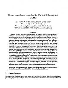
all transition probabilities and used them to simulate the state in question after 15 failed IS proposals. The average IS acceptance rate over all sets of particles and time-points was 16%. Sample averages over the R sets of particles, and, in the case of backward sampling, over the J simulated trajectories for each set of particles, are shown in Figure 1. Obviously all methods provide the same result, which they should, so the differences lie in the variances. 20

15

10

estimate of E(Xk | y0:n)

5

0

−5

−10

−15

−20

−25

0

5

10

15

20

25 k

30

35

40

45

50

Figure 1: Estimates of E[Xk | y1:n ] computed as sample means from the methods GT, GTRB, BS and BSM. The four curves overlap and are not distinguishable. 2 /R for the asymptotic variFor BSM we have the expression σ∞,BSM,k 2 ance, where σ∞,BSM,k is as in Section 3.3; observe that the expression E[h(Xksim ) | ξ (r) ], with h as the identity function, is indeed the mean of Xk obtained with backward smoothing. Here we also include a subindex k as this variance will depend on k, and also a subindex BSM as we will require similar variances for GT and GTRB. For BS we have the asymptotic vari2 )/R as in (3.9), where subindex k in σk2 again denotes ance (σk2 /J + σ∞,BSM,k dependence on time-index k. The asymptotic variances of GT and GTRB 2 2 2 and /R respectively, where σ∞,GT,k /R and σ∞,GTRB,k we write as σ∞,GT,k 2 2 σ∞,GTRB,k are TAVCs defined similarly as σ∞,RB,k but for one trajectory sampled from genealogical tree and for the weighted average over all such

19

trajectories respectively. In practice neither of these variances are known, and we need to estimate them from the simulations. We estimated σk2 by first for each set of particles computing the sample variance of all J trajectories Xksim,j obtained by backward sampling, and then computing the average of these sample variances 2 over all R sets of particles. The TAVCs σ√ ∞ were estimated by summing up estimated autocovariances over lags |ℓ| < R, weighted by (1 − |ℓ|/R) [cf. 5, p. 59]. Inserting these variance estimates into the expressions for asymptotic variances and taking square roots, yield standard errors for the respective estimates of E[Xk | y1:n ], shown in Figure 2. 0.14

0.12

k

standard error of E(X | y

0:n

)

0.1

0.08

0.06

0.04

0.02

0

0

5

10

15

20

25 k

30

35

40

45

50

Figure 2: Standard errors of estimates of E[Xk | y1:n ] for the methods GT (×), GTRB (◦), BS (+) and BSM (∗). We see that GT has standard errors larger than those of BS and BSM, which is to be expected as GT samples a single trajectory while BS samples J = 25 trajectories and BSM averages over all of them. We also see that the standard errors of GT and GTRB are close to identical expect towards the final time-point n. This is a result of the degeneracy of the genealogical tree as for k just a bit less than n there are only one or a few ancestors with descendants alive at time n, and then Rao-Blackwellisation (GTRB) adds little compared to just sampling (GT). For k ≥ 43 say GTRB however does better, and it is on par with BSM for k ≥ 48; for such late time-points 20

the final particles’ ancestries have not coalesced and at time n GTRB and BSM are equivalent. Comparing BS and BSM we find that they have similar standard errors, and this is because the term σk2 /J, with some exceptions k, 2 is smaller than σ∞,BSM,k for J = 25. Comparing standard errors without comparing execution times does not provide the full picture however, and for that reason we introduce a measure of precision per computational effort, defined as inverse variance over computation time. We refer to this measure as efficiency, and we can estimate it using inverse squared standard errors over measured computation times. The computation time of each method was measured using the function cputime in Matlab, the software used for all simulations. Figure 3 plots these estimates. We see that BS is better than BSM, which in turn is better than GT and GTRB which perform about equally. The exception is the last few time-points for which GTRB, which is fast, does very well. The ratios of efficiencies for BS vs. GT (for all k) ranges from 0.19 to 30.7, with 48 (out of 50) of them being larger than one and their geometric mean being 5.4. For BSm vs. GT the corresponding figures are 0.04, 11.4, 36 and 1.8 respectively. 500

450

400

efficiency (1/s)

350

300

250

200

150

100

50

0

0

5

10

15

20

25 k

30

35

40

45

50

Figure 3: Estimated efficiency for estimating E[Xk | y1:n ] for the methods GT (×), GTRB (◦), BS with J = 25 trajectories (+), BS with J = 7 trajectories (∆) and BSM (∗). The y-axis is truncated; GTRB reaches efficiencies about 900 s−1 for the final time points. 21

Having said that, we remark that figures like these crucially depend on software and implementation. GTRB is fast because Matlab does vectorised operations quickly, and we also believe that BS has a slight disadvantage from slow random number generation in Matlab. In addition the resolution of cputime appears to be 10 ms, which may not be short enough to provide accurate measures of execution times (as we measured the time of each call to functions performing the various methods). As discussed in Section 3.3, we can choose the number J of trajectories sampled in the BS method to achieve the best variance/cost performance. This number varies quite a bit with respect to k however, with the minimum value of Jopt (viewed as a continuous variable) being 0.74 and the largest 18.9. As a compromise we chose the geometric mean 6.98, rounded to J = 7 (the arithmetic mean is 8.12). The estimated efficiency for this J is also plotted in Figure 3, and we see that there is improvement over J = 25 that is mostly marginal, but for some k notable. The ratios of efficiencies for this optimised BS vs. GT range from 0.50 to 37.6, with 49 (out of 50) of them being larger than one and their geometric mean being 7.5.

A A.1

Proofs Proof of Theorem 1

To prove the statement we simply carry through the marginalisation. Thus def −ℓ N i let ξ −ℓ k = (ξk )1≤i≤N,i6=ℓ and define ik analogously; the marginal of πn with J0 respect to (ξ0 , . . . , ξnJn , J0 , . . . , Jn ) is then obtained by integrating πnN over

22

(ik , ξ k−jk )nk=0 . We start with integrating over in and ξ n−jn according to πnN (ξ 0 , . . . , ξ n−1 , ξnjn , i1 , . . . , in−1 , j0 , . . . , jn ) XZ πnN (ξ 0 , . . . , ξ n , i1 , . . . , in , j0 , . . . , jn ) dξ n−jn = in

=

φ0:n|n (ξ0j0 , . . . , ξnjn ) N n+1



×

n−1 Y

i

jk

i

jk

k k , ξkjk ) q(ξk−1 ωk−1



 jk ℓ ℓ ) ω q(ξ , ξ ℓ=1 k−1 k−1 k k=1   X Z ψ N (ξ , . . . , ξ , i1 , . . . , in ) n 0 n −jn  × j0 Q n jk jk dξ n N ρ0 (ξ0 ) k=1 Πk (Ik , ξk ) n i−j n   jn ijnn ijnn X ωn−1 q(ξn−1 , ξn )  . (A.1) × PN jn ℓ ℓ ω q(ξ , ξ ) n jn ℓ=1 n−1 n−1 PN

in

In the expression above,

jn

jn

X ijnn

and

in in , ξnjn ) q(ξn−1 ωn−1 jn ℓ ℓ ℓ=1 ωn−1 q(ξn−1 , ξn )

PN

=1

(A.2)

X Z ψ N (ξ , . . . , ξ , i1 , . . . , in ) n 0 n dξ n−jn j0 Q n N (ijk , ξ jk ) ρ (ξ ) Π 0 0 −jn k=1 k k k

in

=

Combining (A.1)–(A.3) yields

ψnN (ξ 0 , . . . , ξ n−1 , i1 , . . . , in−1 ) . (A.3) Qn−1 N jk jk ρ0 (ξ0j0 ) k=1 Πk (ik , ξk )

πnN (ξ 0 , . . . , ξ n−1 , ξnjn , i1 , . . . , in−1 , j0 , . . . , jn ) φ0:n|n (ξ0j0 , . . . , ξnjn ) ψnN (ξ 0 , . . . , ξ n−1 , i1 , . . . , in−1 ) = × Qn−1 N jk jk N n+1 ρ0 (ξ0j0 ) k=1 Πk (ik , ξk ) ×

n−1 Y k=1

i

jk

i

jk

k k , ξkjk ) q(ξk−1 ωk−1

jk ℓ ℓ ℓ=1 ωk−1 q(ξk−1 , ξk )

PN

−j

. (A.4)

n−1 Now, by integrating (A.4) with respect to (in−1 , ξ n−1 ) and repeating the −jn−2 −j1 same procedure for (in−2 , ξ n−2 ), . . . , (i1 , ξ 1 ) and finally ξ 0−j0 we obtain

23

the marginal density πnN (ξ0j0 , . . . , ξnjn , j0 , . . . , jn ) =

φ0:n|n (ξ0j0 , . . . , ξnjn ) . N n+1

(A.5)

Finally, for any rectangle A = A0 × A1 × · · · × An in B(X)(n+1) ,   PπnN ξ0J0 ∈ A0 , . . . , ξnJn ∈ An Z XZ = πnN (ξ0j0 , . . . , ξnjn , j0 , . . . , jn ) dξ0j0 · · · dξnjn = φ0:n|n (A) , ··· j0:n

An

A0

implying that these measures are identical on B(X)(n+1) . We complete the proof by noting that the arguments above apply independently of the particle sample size N .

A.2

Proof of Theorem 2

It is enough to prove that def

R =

πnN (ξ 0 , . . . , ξ n , I1 , . . . , In , J0 , . . . , Jn ) ZnN = , knN (ξ 0 , . . . , ξ n , I1 , . . . , In , J0 , . . . Jn ) Zn

where ZnN is defined in (3.3). Using that I

Jk

I

Jk

k k ϑk−1 ωk−1

Jk Jk ΠN k (Ik , ξk ) = PN

ℓ ℓ ℓ=1 ωk−1 ϑk−1

we obtain

I

Jk

k , ξkJk ) , rk−1 (ξk−1

J P PN Q Ik k ℓ ℓ ℓ φ0:n|n (ξ0J0 , . . . , ξnJn ) nk=1 {q(ξk−1 , ξkJk ) N ℓ=1 ωk−1 ϑk−1 } ℓ=1 ωn R = . J J Q Ik k Jk−1 Jk Ik k , ξkJk )} N n+1 ρ0 (ξ0J0 )ω0J0 nk=1 {ωkJk q(ξk−1 , ξk )ϑk−1 rk−1 (ξk−1 (A.6)

Now, by the definition (3.2) of the importance weights, I

Jk

I

Jk

I

Jk

k k k , ξkJk ) , ξkJk ) = gk (ξkJk )q(ξk−1 rk−1 (ξk−1 ωkJk ϑk−1

(A.7)

and plugging the identity (A.7) into (A.6) gives, using that, in addition, ρ0 (ξ0J0 )ω0J0 = ρ(ξ0J0 )g0 (ξ0J0 ), P Qn PN ℓ ℓ ℓ φ0:n|n (ξ0J0 , . . . , ξnJn ) N ℓ=1 ωn k=1 ℓ=1 ωk−1 ϑk−1 . R= Q Jk−1 Jk N n+1 ρ(ξ0J0 )g0 (ξ0J0 ) nk=1 {gk (ξkJk )q(ξk−1 , ξk )} 24

Finally, we conclude the proof by noting that φ0:n|n (ξ0J0 , . . . , ξnJn )Zn = ρ(ξ0J0 )g0 (ξ0J0 )

n Y

J

k−1 , ξkJk )} . {gk (ξkJk )q(ξk−1

k=1

References [1] Andrieu, C., A. Doucet, and R. Holenstein (2010). Particle Markov chain Monte Carlo methods (with discussion). J. Roy. Statist. Soc. B 72, 269–342. [2] Andrieu, C., A. Doucet, S. S. Sumeetpal, and V. B. Tadi´c (2004). Particle methods for change detection, system identification, and control. Proc. IEEE 92, 423–438. [3] Asmussen, S. and P. W. Glynn (2007). Stochastic Simulation. Algorithms and Analysis. New York: Springer. [4] Baum, L. E., T. P. Petrie, G. Soules, and N. Weiss (1970). A maximization technique occurring in the statistical analysis of probabilistic functions of Markov chains. Ann. Math. Statist. 41 (1), 164–171. [5] Brockwell, P. J. and R. A. Davis (2002). Introduction to Time Series and Forecasting (2nd ed.). Springer. [6] Capp´e, O., E. Moulines, and T. Ryd´en (2005). Inference in Hidden Markov Models. New York: Springer. [7] Chib, S. (1996). Calculating posterior distributions and modal estimates in Markov mixture models. J. Econometrics 75, 79–97. [8] Douc, R., A. Garivier, E. Moulines, and J. Olsson (2011). Sequential Monte Carlo smoothing for general state space hidden Markov models. Ann. Appl. Probab.. to appear. [9] Douc, R., E. Moulines, and J. Olsson (2009). Optimality of the auxiliary particle filter. Probab. Math. Statist. 29 (1), 1–28. [10] Douc, R., E. Moulines, J. Olsson, and R. Van Handel (2011). Consistency of the maximum likelihood estimator for general hidden markov models. The Annals of Statistics. to appear. [11] Doucet, A., N. De Freitas, and N. Gordon (Eds.) (2001). Sequential Monte Carlo Methods in Practice. New York: Springer. 25

[12] Doucet, A., S. Godsill, and C. Andrieu (2000). On sequential MonteCarlo sampling methods for Bayesian filtering. Stat. Comput. 10, 197–208. [13] Durbin, R. and S. J. Koopman (2001). Time Series Analaysis by State Space Methods. Oxford: Oxford University Press. [14] Fearnhead, P. (1998). Sequential Monte Carlo methods in filter theory. Ph. D. thesis, University of Oxford. [15] Gustafsson, F. (2010). Particle filter theory and practice with positioning applications. IEEE Aerospace Electronic Syst. Mag. 25, 53–82. [16] Olsson, J., T. Ryd´en, and S. Stjernqvist (2010). A particle-based Markov chain Monte Carlo sampler for state-space models with applications to DNA copy number data. Submitted. Also appears in S. Stjernqvist’s PhD thesis Modelling Allelic and DNA Copy Number Variations Using Continuous-Index Hidden Markov Models, Centre for Mathematical Sciences, Lund University, 2010. [17] Pitt, M. K. and N. Shephard (1999). Filtering via simulation: auxiliary particle filters. J. Am. Statist. Assoc. 94 (446), 590–599. [18] Robert, C. P., G. Celeux, and J. Diebolt (1993). Bayesian estimation of hidden Markov chains: a stochastic implementation. Statist. Probab. Lett. 16, 77–83. [19] Roberts, G. O. and J. S. Rosenthal (2004). General state space Markov chains and MCMC algorithms. Probab. Surv. 1, 20–71. [20] Sch¨ on, T., F. Gustafsson, and R. Karlsson (2011). Particle filtering in practice. In D. Crisan and B. L. Rozovskii (Eds.), Oxford Handbook of Nonlinear Filtering. Oxford University Press. to appear.

26