Article
Microelectromechanical Resonant Accelerometer Designed with a High Sensitivity Jing Zhang, Yan Su † , Qin Shi † and An-Ping Qiu * Received: 11 October 2015; Accepted: 25 November 2015; Published: 3 December 2015 Academic Editor: Stefano Mariani School of Mechanical Engineering, Nanjing University of Science and Technology, Nanjing 210094, China;
[email protected] (J.Z.);
[email protected] (Y.S.);
[email protected] (Q.S.) * Correspondence:
[email protected]; Tel.: +86-133-8208-3366; Fax: +86-25-843-0325-8806 † These authors contributed equally to this work.
Abstract: This paper describes the design and experimental evaluation of a silicon micro-machined resonant accelerometer (SMRA). This type of accelerometer works on the principle that a proof mass under acceleration applies force to two double-ended tuning fork (DETF) resonators, and the frequency output of two DETFs exhibits a differential shift. The dies of an SMRA are fabricated using silicon-on-insulator (SOI) processing and wafer-level vacuum packaging. This research aims to design a high-sensitivity SMRA because a high sensitivity allows for the acceleration signal to be easily demodulated by frequency counting techniques and decreases the noise level. This study applies the energy-consumed concept and the Nelder-Mead algorithm in the SMRA to address the design issues and further increase its sensitivity. Using this novel method, the sensitivity of the SMRA has been increased by 66.1%, which attributes to both the re-designed DETF and the reduced energy loss on the micro-lever. The results of both the closed-form and finite-element analyses are described and are in agreement with one another. A resonant frequency of approximately 22 kHz, a frequency sensitivity of over 250 Hz per g, a one-hour bias stability of 55 µg, a bias repeatability (1σ) of 48 µg and the bias-instability of 4.8 µg have been achieved. Keywords: resonant accelerometer; SOI; micro-lever mechanism; sensitivity; MEMS
1. Introduction Microelectromechanical accelerometers can be found in numerous applications such as inertial navigation systems, gaming, smartphones and mobile devices [1]. These devices are very attractive for high-precision measurement applications due to their high sensitivity, frequency output and large dynamic range [2–4]. In a silicon micro-machined resonant accelerometer (SMRA), the acceleration is measured through the differential frequency shift originated by axial loading between the two pull and push double-ended tuning fork (DETF) resonators. This type of resonant accelerometer benefits from a direct frequency shift between the resonators when sensing the input acceleration and this feature draws the extensive attention of researchers. The sensitivity of the SMRA is defined as the differential output frequency of the resonators produced by an acceleration of 1 g. It is an important characteristic and deserves to be researched. A high sensitivity allows for the acceleration signal to be easily demodulated by frequency counting techniques [2] and decreases the overall noise on the readout electronics [5]. Recently, the design and fabrication of various mechanical resonant accelerometers have been studied [1,6,7]. Pinto et al., have presented the design of a very small and sensitive resonant accelerometer [4]. By using thin silicon-on-insulator (SOI)-based technologies compatible with “In-IC“ integration, the accelerometer size has been reduced drastically (0.05 mm2 ˆ 4.2 µm) with a sensitivity of 22 Hz/g. Sandia
Sensors 2015, 15, 30293–30310; doi:10.3390/s151229803
www.mdpi.com/journal/sensors
Sensors 2015, 15, 30293–30310
National Laboratories have developed an in-plane microelectromechanical systems (MEMS)-based nano-g accelerometer with a subwavelength optical resonant sensor in [8], where the authors focus on the maximum mass and the minimum spring constant to achieve a high sensitivity of 590 V/g ‘ and resolution of 17 ng/ Hz. Zou et al., optimized a tilt accelerometer to obtain a design trade-off between sensitivity, resolution and robustness [9,10]. However, each part of this sensitive structure was optimized separately without considering the interaction effect between each other. Su et al., designed a two-stage micro-leverage mechanism in the silicon resonant accelerometer and provided the theory for the amplification factor of the micro-leverage [11]. Constraint conditions have great effect on the amplification efficiency of the micro levers, but this study did not take these factors into consideration. Although many of these studies have been concerned with the structure of resonant accelerometers to improve the ability to sense accelerations, their methods for the design and the sensitivity achievable from such sensors still remain limited. There remains a need for an efficient and systematic method that can obtain a reasonable structure with a high sensitivity based on the trade-off between the geometry of the accelerometer and its fabrication requirements. This paper will show an in-plane SMRA by building upon previous work [5,12–14]. However, the geometrical setting, and hence, the properties of the mechanical parts are different. The structure of an SMRA is regarded as an energy transmission system, and each part consumes and transmits energy. Our study applies the energy-consumed concept to the SMRA to address the design issues and to increase its sensitivity. This sensor is referred to as a compliant mechanism. Based on the law of the conservation of energy, micro-lever mechanisms with boundary conditions are optimized to consume low energy and to show high force transmission efficiency between the proof mass and the resonators. This is very important for the design of resonant accelerometers. Currently, such an application of the energy-consumed concept has not been reported. In addition, the Nelder-Mead method [15,16] with constraint conditions is initially used as the optimization algorithm. The SOI processing has an integrated 80 µm-thick single-crystal silicon structure with a standard on-chip circuit. It offers a higher aspect ratio MEMS structure that will reduce the cross-axis sensitivity and increase the robustness of the sensors [17]. This paper demonstrates an SMRA with a 211.5 Hz/g nominal sensitivity (66.1% higher than the previous structure), one-hour bias stability of 55 µg and a bias repeatability of 48 µg. The device possesses a good output frequency nonlinearity of within ˘40 g input acceleration (corresponding over the 16 kHz output frequency shift of the resonators). A very good agreement is obtained between the results of the closed-form analyses and those of the finite-element analyses. In what follows, we report on the experimental characterization of an SMRA based on the resonant sensing principles [2]. This paper is organized as follows: Section 2 describes the operation principle and the SOI processing for the SMRA dies, Section 3 proposes the reasonable design for each part of the SMRA and how to obtain an optimum sensitivity, Section 4 presents simulated and experimental results to compare with the theoretical predictions, and Section 5 contains the conclusions of the entire work. 2. Background 2.1. Operation Principle The SMRA structure is shown as a schematic in Figure 1. This structure can be divided into four major components: a proof mass, micro levers, flexure suspensions and DETFs. All these components have coplanar faces. Two DETFs are joined via micro-levers to the proof mass. The proof mass is constrained to move along the y-axis by four flexures, which are linked to the frame mounted to the silicon substrate by four anchors. When acceleration along the input axis is applied to the device, the force from the proof mass is magnified by micro-lever and then transferred to the DETFs. This input applies axial loads, either tension or compression, to the DETFs, which produces a measurable natural frequency shift between the two resonators. The output of the SMRA is the differential frequency
30294
Sensors 2015, 15, 30293–30310
variation of the two resonators, and this differential arrangement enables a first-order cancellation of Sensors 2015,parasitic 15, page–page common sensitivities such as temperature. DETF resonator 1
DETF resonator
Frame
Connecting mass 1
Micro-leverage mechanism
Acceleration Input Axis
Connet beam Connecting mass 1
Proof mass
Flexure
pivot beam output beam lever arm
input beam
Flexure
lb1
Connecting mass 1
la
DETF resonator 2
lb2
y z
x Fixed
Free
Figure 1. Schematic view of the SMRA with a frame structure. Figure 1. Schematic view of the SMRA with a frame structure.
2.2. Dies Based on the SOI-MEMS Process 2.2. Dies Based on the SOI-MEMS Process The SMRA has been fabricated with SOI processing and wafer-level vacuum packaging [18]. The SMRA has been fabricated with SOI processing and wafer-level vacuum packaging [18]. The main characteristic of the SOI process is the use of silicon-to-silicon direct bonding (SSDB) and The main characteristic of the SOI process is the use of silicon-to-silicon direct bonding (SSDB) and high-aspect ratio inductively coupled plasma (ICP) etching technology [17,19]. This process offers high-aspect ratio inductively coupled plasma (ICP) etching technology [17,19]. This process offers an 80 μm-thick MEMS structure with a high aspect ratio up to 1:30, which will then reduce an 80 µm-thick MEMS structure with a high aspect ratio up to 1:30, which will then reduce cross-axis cross-axis sensitivity and increase the robustness of the sensors. sensitivity and increase the robustness of the sensors. The process cross-section is schematically represented in Figure 2. The die is realized with The process cross-section is schematically represented in Figure 2. The die is realized with three three wafers, the substrate, the SOI device layer and the cover. The sensor surface is around wafers, the substrate, the SOI device layer and the cover. The sensor surface is around 110 mm2 and 110 mm2 and its thickness for the three layers is 700 μm. The SOI device layer is 80 μm thick and is its thickness for the three layers is 700 µm. The SOI device layer is 80 µm thick and is manufactured manufactured using deep reactive ion etching on the SOI wafer with a high aspect ratio of up to using deep reactive ion etching on the SOI wafer with a high aspect ratio of up to 1:30. The residual 1:30. The residual stress is much less than that of a silicon-on-glass (SOG) process [20]. The cover stress is much less than that of a silicon-on-glass (SOG) process [20]. The cover and the active SOI and the active SOI layer are joined by an Au/Si eutectic bonding, forming a hermetic cavity that layer are joined by an Au/Si eutectic bonding, forming a hermetic cavity that maintains the vacuum maintains the vacuum needed for a high-Q operation of the SMRA. To maintain the vacuum level needed for a high-Q operation of the SMRA. To maintain the vacuum level over the long term, a getter over the long term, a getter is adhered to the inner surface of the cover, and once it is activated, the is adhered to the inner surface of the cover, and once it is activated, the getter progressively absorbs getter progressively absorbs and traps gaseous species. The packaged SMRA die was placed in a and traps gaseous species. The packaged SMRA die was placed in a ceramic cartridge to protect the ceramic cartridge to protect the silicon structure and to facilitate the welding of the whole device. silicon structure and to facilitate the welding of the whole device. Figure 3 shows the wafer-level Figure 3 shows the wafer-level vacuum packaged SMRA dies, and Figure 4 shows the SEM vacuum packaged SMRA dies, and Figure 4 shows the SEM (Scanning Electron Microscope) photo of (Scanning Electron Microscope) photo of the SMRA structure. The vacuum level of the sensor is the SMRA structure. The vacuum level of the sensor is measured at 10 Pa. measured at 10 Pa.
Cover SOI device Substrate
Silicon
Silicon dioxide
Au
30295 Figure 2. SOI-MEMS (silicon-on-insulator microelectromechanical system) process cross-section of the die.
getter progressively absorbs and traps gaseous species. The packaged SMRA die was placed in a ceramic cartridge to protect the silicon structure and to facilitate the welding of the whole device. Figure 3 shows the wafer-level vacuum packaged SMRA dies, and Figure 4 shows the SEM (Scanning Electron Microscope) photo of the SMRA structure. The vacuum level of the sensor is Sensors 2015, 15, 30293–30310 measured at 10 Pa.
Cover SOI device Substrate
Silicon
Silicon dioxide
Au
Figure 2. SOI-MEMS (silicon-on-insulatormicroelectromechanical microelectromechanical system) Figure 2. SOI-MEMS (silicon-on-insulator system) process processcross-section cross-sectionofof the die. Sensors 2015, 2015, 15, page–page page–page the die. Sensors 15,
3
Ceramic Ceramic cartridge cartridge
Lead pad Silicon cover
y z
2000 m 2000
x
Figure 3. Photo ofofthe vacuumpackaged packaged Figure 3. Photo theSMRA SMRA wafer-level wafer-level vacuum die.die. resonantor resonantor frame frame connect mass mass 1 1 connect
flexure flexure proof mass mass proof micro-leverage micro-leverage
connect mass mass 2 2 connect 500 m 500
Figure SEM photoof ofthe the mechanical mechanical sensitive Figure 4. 4. SEM photo sensitivestructure. structure.
3. Device Design 3.1. Theoretical Analysis
30296
For each DETF, the natural frequency of the basic lateral vibration mode is expressed as [21] 33
w
33
w
Sensors 2015, 15, 30293–30310
3. Device Design 3.1. Theoretical Analysis For each DETF, the natural frequency of the basic lateral vibration mode is expressed as [21] g g f f ´ w ¯3 ´ w ¯3 f f f f 16.55Et 16.55E 1 e 1 e l l f0 “ “ 2π 0.397ρwtl ` ρqs t 2π 0.397ρwl ` ρqs
(1)
where E is the Young’s modulus, ρ is the density of single-crystal silicon and l, w and t are the length, width and thickness of the resonant beam, respectively. The comb-drive structure and the resonant beam have the same thickness, and qs is the x-y plane area of the comb-drive structure. If qs is constant, it is clear that the natural frequency of one resonant beam depends on the length and the width but is independent of the thickness of the beam. When the acceleration a along the sensitive axis is applied (see Figure 1), the proof mass is subjected to the force F1 = m1 a, and each of the connecting masses is subjected to F2 = m2 a. The axial force on each resonant beam has been magnified by the micro-lever to be ˙ ˆ ˚ A m1 a m2 a ` F“´ 4 2
(2)
where A˚ is the amplification factor of the sensitive structure (i.e., the effective amplification factor) and m1 and m2 are the mass of the proof mass and the connecting mass. Therefore, the resonant beam frequency f under acceleration can be found by energy analysis [22] to be g f d d f 16.55Etp w q3 ˘ 4.85 F ˚ 2 e K 1 1 ef f l l “ f 1 ˘ 0.073 pA m1 ` 2m2 q al f “ “ (3) 0 3 2π Me f f 2π 0.397ρwtl ` ms Ew t where Me f f is the effective mass and Ke f f is the axial effective stiffness of the DETF. 0.073 pA˚ m1 ` 2m2 q al 2 Setting α “ , the frequency shift between two DETFs is Ew3 t ? ? 1 ∆ f “ f 0 1 ` α ´ f 0 1 ´ α “ f 0 α ` f 0 α3 8
(4)
By substituting a = ng (where n is the applied acceleration in terms of g) into Equation (4) and by taking the derivative of ∆f with respect to n, the sensitivity can be expressed in terms of frequency (with units of Hz/g) Sg
d∆ f 0.073 pA˚ q1 ` 2q2 q ρl 2 « f0 g dn Ew3 d l pA˚ m1 ` 2m2 q g “ 0.0473 p0.397ρwtl ` ms q Ew3 t
“
(5)
“ Sres pA˚ m1 g ` 2m2 gq
where Sres is the sensitivity of the DETF sensing element. d Sres “ 0.0473
l p0.397ρwtl ` ms q Ew3 t
30297
(6)
Sensors 2015, 15, 30293–30310
3.2. Effective Amplification Factor A* When acceleration a along the input axis is applied to the device, the force from the proof mass is magnified by the micro-lever and then transferred to the DETFs. The effective amplification factor A˚ is therefore defined as the ratio of the axial force of the DETF beam to the input inertial force of the proof mass. Because the structure is symmetrical with respect to both the x- and y-axes, only one-quarter of the structure has been directly analyzed. Figure 5a shows the model and deformation of each part of the half structure under an inertial load a. All the deformations have been exaggerated for clarity. Because the connecting mass is symmetrical with respect to the y-axis, the bending moment and the horizontal force transferred from output beams will be counteracted. As a result, only the axial force can be transferred to the DETFs and will therefore cause vertical displacements. Figure 5b shows the equivalent model of a quarter of the structure. By supposing the flexure can be regarded as a vertical spring K1 , half of the connecting mass and one DETF can be regarded as vertical springs of which stiffness are k f and kb . By solving the boundary conditions for Fxi , Fyi , Mi , Fyo , Fxo and Mo (see Appendix A), the effective amplification factor can be obtained to be A˚ “
Fyo m1 a{4
(7)
Because this is a fairly large output, the expression for A* is shown in Appendix A. Based on the analysis above, the sensitive structure should be designed to produce a high effective amplification Sensors 15, page–page factor2015, A* , which proportionally contributes to the sensitivity.
M
Euler Bernouli
DETF beams
Timoshenko
kf
Fyo
Connecting mass
wb
5
lout
lin
kb
M o Fyo
Lb
Output beam
Pivot beam
Input beam
lin
3
Fxo
eff
lout
4
2 1
Flexure
Flexure
Fxi
y
a
Fyi M i
K1
x Proof mass
(b)
(a)
Figure the micro-leverage micro-leveragemechanism; mechanism;(b)(b)The The equivalent micro Figure 5. 5. (a) (a) Deformation Deformation of of the equivalent micro leverlever under loading under loading
By substituting Equation (A8) into Equation (A12), we obtain By substituting Equation (A8) into Equation (A12), we obtain
Fyo Fyo d yi Alever Klever Klever Fyo Fyo {dyi Alever A “ F K d “ F d K“ K yi 1 yi yi yi 1 lever F `K d F {d ` K K `KK1 *
˚A
yi
1 yi
yi
yi
1
lever
(8)
(8)
1
where = Fyo/Fyi represents the amplification factor of the micro-lever, and Klever = Fyi/dyi represents where AAlever lever = Fyo /Fyi represents the amplification factor of the micro-lever, and Klever = Fyi /dyi the spring the constant the micro-lever. Both ABoth lever and Klever are decided by the geometry of the represents spring of constant of the micro-lever. Alever and Klever are decided by the geometry * micro-lever, and K 1 has no influence on them; therefore, the effective amplification factor of the micro-lever, and K1 has no influence on them; therefore, the effective amplification factor A˚ A increases asK1Kdecreases. 1 decreases. Asthe forconnecting the connecting mass, be it rigid should be rigid to conservation ensure energy increases as As for mass, it should to ensure energy conservation in an ideal situation. In reality, if kb is 10 times greater than kf, the connecting mass can be regarded as rigid. The design for the connecting mass relies on this principle. 3.3. DETF Design Analysis
30298
The corresponding enhancement to the sensitivity owes not only to micro-lever mechanisms’ reasonable design, but also to the reasonable design for the resonators. As shown in Equation (6),
A
Fyi K1d yi
Fyi d yi K1
(8)
Klever K1
where Alever = Fyo/Fyi represents the amplification factor of the micro-lever, and Klever = Fyi/dyi represents the spring constant of the micro-lever. Both Alever and Klever are decided by the geometry of the micro-lever, and K1 has no influence on them; therefore, the effective amplification factor A* Sensors 2015, 15, 30293–30310 increases as K1 decreases. As for the connecting mass, it should be rigid to ensure energy conservation in an ideal situation. In reality, if kb is 10 times greater than kf, the connecting mass can in an ideal situation. In reality, if k is 10 times greater than k f , the connecting mass can be regarded be regarded as rigid. The design forb the connecting mass relies on this principle. as rigid. The design for the connecting mass relies on this principle.
3.3.3.3. DETF Design DETF DesignAnalysis Analysis The corresponding owes not notonly onlytotomicro-lever micro-levermechanisms’ mechanisms’ The correspondingenhancement enhancement to to the the sensitivity sensitivity owes reasonable thereasonable reasonabledesign design resonators. As shown in Equation reasonabledesign, design,but butalso also to to the forfor thethe resonators. As shown in Equation (6), the(6), thesensitivity sensitivity of DETF res increases an increase to thelength beamand length and decreases with an of DETF Sres Sincreases with with an increase to the beam decreases with an increase increase to thewidth. beam Figure width. 6Figure shows the variation trend Sres: the sensitivity of DETF to the beam shows 6the variation trend of Sres : theofsensitivity of DETF increases steadily steadily when thewhen beam length changes fromchanges 300 µm to 1100300 µm,μm while decreases the increases the beam length from to it1100 μm, rapidly while itwhen decreases beam width from 1 µmchanges to 10 µm, especially 3 µm. Thinner, longer beams rapidly when changes the beam width from 1 μm when to 10 less μm,than especially when less than 3 μm. providelonger more sensitivity, but may alsosensitivity, cause resonator mismatch due toresonator process, with detrimental Thinner, beams provide more but may also cause mismatch due to effects with to thedetrimental temperatureeffects stabilitytoofthe thetemperature sensor. This is a trade-off in the mechanical design, process, stability of the sensor. This isstructure a trade-off in the and the optimum geometry of DETF will be point out in next section. mechanical structure design, and the optimum geometry of DETF will be point out in next section. 6
5
x 10
8
x 10
Resonant beam lenth:
Resonant beam width:
650 micron 761.5 micron 900 micron
7
4.5 micron 5.5 micron 6.5 micron
7
Sensitivity of DETF Sres (Hz/N/g)
Sensitivity of DETF Sres (Hz/N/g)
8
6
5
4
6 5
x 10 9
5
8 7
4
6 5 4
3
3 2
2
1 5
3
2 200
5.5
6
6.5
7
7.5
8
1
300
400
500
600
700
800
900
1000
1100
0 1
1200
Length of DETF beam (μm)
(a)
2
3
4
5 6 Width of DETF beam (μm)
7
8
9
10
(b)
Figure 6. 6. (a)(a) Sres asas a function for aaseries seriesofofbeam beamwidths; widths; and Figure Sres a functionofofthe theDETF DETF beam beam length length for and (b)(b) SresSres as as a a function of the DETF beam width for a series of beam lengths. function of the DETF beam width for a series of beam lengths.
6
3.4. Reasonable Design of the Structure
By substituting Equation (7) into Equation (5), there is a tremendous dimension system about the sensitivity Sg . To obtain a high Sg , the Nelder-Mead method under constraint conditions is used as the optimization algorithm for each part of the SMRA. The Nelder-Mead method is a technique for minimizing an objective function in multidimensional space. It uses the concept of a simplex, which is a special polyhedron with N + 1~2N vertexes in N dimensions [16]. In this paper, the energy-consumed concept (energy-consumed concept: based on the conservation of energy law, micro-lever mechanisms with boundary conditions are optimized to consume a low amount of energy and show high-force transmission efficiency from the proof mass to the resonators) is applied to this method and used as the structure optimization algorithm. The flow chart for this algorithm under constraint conditions is shown in Figure 7. The sensitivity is regarded as the negative objective function to obtain a maximum result. Limited by the layout size, the proof mass area is assumed to be lower than 8 mm2 . The first vibrating mode (the first mode: when SMRA is under acceleration, the proof mass will generate an inertial force, amplified by the micro-lever mechanism; then, the amplified inertial force will cause axial push and pull loading on the DETF resonators) frequency can be expressed as d f1 “
4 pKlever ` K1 q m1
30299
(9)
mechanism; then, the amplified inertial force will cause axial push and pull loading on the DETF resonators) frequency can be expressed as
f1
Sensors 2015, 15, 30293–30310
4 Klever K1
(9)
m1
START
INPUT DATA
END
calculate accuracy YES NO
Set objective function J f ( x0 , x1 , , xn 1 ) Create constant constraints ① ai xi bi , i 0,1, , n 1 Create function constraints ② Ck ( x0 , x1 , , xn 1 ) Wk ( x0 , x1 , , xn 1 ) Dk ( x0 , x1 , , xn 1 )
2 1 2n fi f ( X T ) 2n i 1
1
2
j 1
k 0,1, , m 1 x M X T , f M f ( X T )
INPUT DATA:Coordinates of the initial vertex
f j f ( x j )
YES
x 0 ( x00 , x10 , , xn 10 )
f j f M
x 0satisfies the constraints ①and②
NO
YES
NO
XT X F XT 2
f M f j f R YES
NO
X T satisfies
the constraints ②
NO YES
f M f j , M j
f R f j , R j X T ,i ai , 106
j j 1
or
NO
X T satisfies
the constraints ①
X T ,i bi
j=1, f 0 f ( x 0 ), f M f R f 0
YES
j 2n 1 NO
YES
Repeat loop
XT X F XT 2
Create vertex x j ( x0 j , x1 j , , xn 1 j ), where xij ai r (bi ai ), i 0,1, , n 1 and r is a pseudorandom number from 0 to 1.
x j x j T
where T NO
NO
f X T f R
X T 1 X F x M
where X F
1 2 n 1 x 2n 1 k 0 k
and 1.2 2.0
2
1 j 1 x j 1 k 1 k
x 0satisfies the
YES Repeat loop
constraints ②
Figure 7. Flow chart for the Nelder-Mead method under constraint conditions. Figure 7. Flow chart for the Nelder-Mead method under constraint conditions.
In the testing environment, the first mode frequency should be larger than 2.1 kHz to stay away from low-frequency external vibrations. Substituting m1 into Equation (9), the spring constant K1 + Klever is assumed to be more than 71.4 N/m. The width of each beam is assumed to be equal to or larger than 4.5 µm which is limited by the processing level. Therefore, the range of each beam’s geometry is set as shown in Table 1 for our design requirements. Because kb is assumed to be 10 times greater than k f , the connecting mass can be regarded as rigid, which helps to reduce the energy 7 consumed. All the above requirements are used as constraint conditions for the Nelder-Mead method. The SMRA geometric dimensions after optimization are shown in Table 1. Its sensitivity is determined to be 216.35 Hz/g. Limiting by the layout size and processing level and based on the energy-consumed concept, several dimensions have been corrected slightly. The final sensitivity is 211.5 Hz/g, 66.1% higher than the previous structure’s sensitivity of 127.33 Hz/g [14]. The FEM (finite-element analyses) result of the first vibrating mode is 1994.59 Hz, 4.7% lower than the theoretical value of 2.1 kHz. Meanwhile, the energy consumed in each component of this sensitive structure is shown in Table 2. The DETF in this work consumes 59.6% of the total energy, while the DETF of the earlier structure consumes only 6.58 ppm (parts per million). Table 3 shows the ratio of the sensitivity improvement contributed by the DETF, the new micro-lever and the proof mass. This means that the sensitivity improvement is mainly attributed to both the re-designed DETF and the reduced energy loss on the lever. The micro-lever mechanisms (given the boundary conditions) consume lower energy and show high force transmission efficiency from the proof mass to the DETF resonators. If another optimum sensitivity is required, users can simply change the constraint conditions of the Nelder-Mead algorithm and repeat the steps above.
30300
Sensors 2015, 15, 30293–30310
Table 1. Sensitive Structure Dimensions of the SMRA compared to earlier structure. Variable
lr (µm)
wr (µm)
li (µm)
wi (µm)
lo (µm)
wo (µm)
lp (µm)
wp (µm)
Size range
100–1500
5.5–8
50–480
4.5–10
20–350
4.5–10
10–350
4.5–10
lin (µm)
lout (µm)
200–1650 >(wo + w p )/2
wc (µm)
Lc (µm)
la (µm)
lb1 (µm)
lb2 (µm)
lin /10 < wc < lin /2
2lin -10
9–20
200–1000
Lb1 –20
Optimal value
761.4
5.5
242.2
5.63
44.8
5.24
196.1
4.5
1641
54.9
1225
3272
10.7
390.3
370.3
Corrected value
761.5
5.5
242
5.5
45
5
196
4.5
900
29
525
1700
11
390
370
Earlier structure
1000
8
300
6
60
4
270
6
644
19
–
–
16
650
650
* l and w, respectively, represent length and width. r, i, o and p represent the length of the resonant beam, input beam, output system and pivot beam, respectively.
30301
Sensors 2015, 15, 30293–30310
Table 2. Energy consumed in each component of the SMRA. Energy Consume ˆ 10´17 a2 (J)
Component
Earlier Structure DETF Flexure Input beam Output beam Pivot beam Lever arm(in) Lever arm(out) Connecting mass
This Work
10´4
Earlier Structure 10´4
24.56 6.51 2.19 1.09 1.04 2.55 0.07 3.27
7.96 ˆ 41.93 51.69 23.35 3.825 0.24 9.47 ˆ 10´5 8.8 ˆ 10´4
Ratio (%)
6.58 ˆ 34.64 42.71 19.3 3.16 0.198 7.82 ˆ 10´7 7.27 ˆ 10´6
This work 59.6 15.8 5.3 2.6 2.5 6.2 0.2 7.9
Table 3. The sensitivity improvement between the two work.
SMRA
Sensitivity of DETF (Hz/N)
Effective Amplification Factor A*
The Proof Mass (kg)
Sg (Hz/g)
Previous design This work Ratio for the improvement
399,393 490,303 22.8%
22.04 26.67 21%
1.42 ˆ 10´6 1.7 ˆ 10´6 19.72%
127.33 211.5 66%
4. Simulation and Experiments for the SMRA The micro-lever mechanism can be evaluated by the output frequency by supposing one resonator’s natural frequency is f 10 . When it is subjected to an inertial force, the frequency becomes f 1 . By substituting f 10 into Equation (1) and f 1 into Equation (3), we obtain 2 “ f 12 ´ f 10
2 pA˚ q ` 2q q ρal 2 0.073 f 10 2 1 Ew3
(10)
0.073ρal 2 , the effective amplification factor A˚ for one resonator can be determine Ew3 by Equation (10) as follows: f 2 { f 2 ´ p1 ` 2q2 cq A˚ “ 1 10 (11) q1 c By setting c “
Equation (11) can be used to judge whether the design of the micro-lever mechanism is reasonable. The SMRA has been simulated by FEA software, from which the sensitive structure was subjected to an input acceleration in the range of ˘40 g (see Figure 8). By fitting 13 datasets, the output frequency, simulated frequency and sensitivity agree with the designed values, as shown in Table 4. Moreover, the effective amplification factor is calculated through Equation (11). The nonlinearity of Sg within ˘40 g is 49.66 ppm (parts per million).
30302
The SMRA has been simulated by FEA software, from which the sensitive structure was subjected to an input acceleration in the range of ±40 g (see Figure 8). By fitting 13 datasets, the output frequency, simulated frequency and sensitivity agree with the designed values, as shown in Table 4. Moreover, the effective amplification factor is calculated through Equation (11). The Sensors 2015, 15, 30293–30310 nonlinearity of Sg within ±40 g is 49.66 ppm (parts per million). 30000
f1 f2 Linear Fit of Frec/Hz Linear Fit of D
28000
Frec/Hz
26000
24000
Equation y = a + b*x Value Standard f1/Hz Intercep 25450.54 28.96409 Slope 101.4988 1.18245 f2/Hz Intercep 25462.37 32.28081 Slope -101.498 1.31786
22000
20000 -40
-20
0
20
40
a/g
Figure Figure8.8.Simulated Simulatedresonant resonantfrequency frequencyoutput outputversus versusthe the input input acceleration. acceleration. Table Table 4. 4. Simulated Simulatedand andtesting testing results results of of the the SMRA. SMRA.
Results and Errors Results andresults Errors Theory Simulated values Theory results Relative shift Simulated values Relative shift
f0 (Hz) Effective Amplification Factor A* f0 Effective Amplification 26,053.5 26.2A˚ (Hz) Factor 25,585.4 26.67/25.33 26,053.5 26.2 1.8% 1.88%/3.33% 25,585.4 26.67/25.33 1.8%
1.88%/3.33%
Sg (Hz/g) Sg 211.5 (Hz/g) 203 211.5 4.19% 203 4.19%
The initial testing was performed in open air at the Sci & Tech Micro Inertial Technology Lab of the Nanjing University. Three SMRA prototypes (A1-5, A1-7, and A1-8) had been chosen for The initial testing was performed in open air at the Sci & Tech Micro Inertial Technology Lab of testing these prototypes adopted a self-excited oscillation loop with automatic gain control (AGC) the Nanjing University. Three SMRA prototypes (A1-5, A1-7, and A1-8) had been chosen for testing as the drive circuit, and the packaged SMRA dies were finally placed in a ceramic cartridge. The these prototypes adopted a self-excited oscillation loop with automatic gain control (AGC) as the ceramic cartridge package was put on a socket that was wire-connected to an off-chip circuit on a drive circuit, and the packaged SMRA dies were finally placed in a ceramic cartridge. The ceramic PC board. During our testing, the output was connected to an oscilloscope. Without any input cartridge package was put on a socket that was wire-connected to an off-chip circuit on a PC board. acceleration in A1-5, the resonant frequency of one DETF was 22,447.45 Hz and that of the other During our testing, the output was connected to an oscilloscope. Without any input acceleration DETF was 22,179.4 Hz. The gaps between the normalized frequencies are attributed to thermal in A1-5, the resonant frequency of one DETF was 22,447.45 Hz and that of the other DETF was and residual stress during the process. Substituting the measured frequency into Equation (5), the 22,179.4 Hz. The gaps between the normalized frequencies are attributed to thermal and residual theoretical sensitivity is determined to be 249.46 Hz/g. stress during the process. Substituting the measured frequency into Equation (5), the theoretical The PC board of A1-5 was then placed vertically on a rotating platform with a constant sensitivity is determined to be 249.46 Hz/g. temperature control. When this prototype was subjected to 1 g, the resonant frequency for the pull The PC board of A1-5 was then placed vertically on a rotating platform with a constant resonator was 22,574.23 Hz, while the push resonator was 22,047.41 Hz. The increased frequency of temperature control. When this prototype was subjected to 1 g, the resonant frequency for the pull 2 resonator was 22,574.23 Hz, while the push resonator was 22,047.41 Hz. The increased frequency of the pull resonator was 126.78 Hz, and the decreased frequency of the push resonator was 131.99 Hz. The total frequency shift was therefore translated to a sensitivity of 258.77 Hz/g, only 3.6% higher than the calculation of 249.46 Hz/g. Figure 9 shows experimental points and a linear fitting of the measured differential frequency for the acceleration of sin(θ) g on the three SMRA prototypes: A1-5, A1-7, A1-8. The rotating angle θ was adjusted to be 0˝ , 5˝ , 15˝ , 25˝ , 45˝ , 65˝ , 75˝ , 85˝ , 90˝ , 95˝ , 105˝ , 115˝ , 135˝ , 155˝ , 165˝ , 175˝ , 180˝ , 185˝ , 195˝ , 205˝ , 225˝ , 245˝ , 255˝ , 265˝ , 270˝ , 275˝ , 285˝ , 295˝ , 315˝ , 335˝ , 345˝ , and 355˝ , respectively [23]. Good linearity of these prototypes is observed in this range of operation. By fitting the 32 sets of the differential frequency, the average sensitivity within 1 g turns out to be 254.3 Hz/g. As shown in Figure 10, when the SMRA prototypes were subjected to an input acceleration in the range of ˘40 g with a constant temperature control, the testing nonlinearity of the sensitivity is within 100 ppm. All of the above results have helped to confirm our theory. 30303
θ was adjusted to be 0°, 5°, 15°, 25°, 45°, 65°, 75°, 85°, 90°, 95°, 105°, 115°, 135°, 155°, 165°, 175°, 180°, 185°, 195°, 205°, 225°, 245°, 255°, 265°, 270°, 275°, 285°, 295°, 315°, 335°, 345°, and 355°, 180°, 185°, 195°, 205°, 225°, 245°, 255°, 265°, 270°, 275°, 285°, 295°, 315°, 335°, 345°, and 355°, respectively [23]. Good linearity of these prototypes is observed in this range of operation. By fitting respectively [23]. Good linearity of these prototypes is observed in this range of operation. By fitting the 32 sets of the differential frequency, the average sensitivity within 1 g turns out to be 254.3 Hz/g. the 32 sets of the differential frequency, the average sensitivity within 1 g turns out to be 254.3 Hz/g. As shown in Figure 10, when the SMRA prototypes were subjected to an input acceleration in the As shown in Figure 10, when the SMRA prototypes were subjected to an input acceleration in the range 2015, of ±40 g with a constant temperature control, the testing nonlinearity of the sensitivity is Sensors 15, 30293–30310 range of ±40 g with a constant temperature control, the testing nonlinearity of the sensitivity is within 100 ppm. All of the above results have helped to confirm our theory. within 100 ppm. All of the above results have helped to confirm our theory. 300 300
Differential Frec/Hz Differential Frec/Hz
200 200 100 100
A1-5 A1-5 A1-7 A1-7 A1-8 A1-8 Linear fit of A1-5 Linear Linear fit fit of of A1-5 A1-7 Linear Linear fit fit of of A1-7 A1-8 Linear fit of A1-8
0 0
Equation Equation Residual S Residual S Linear Fit Linear A1-5 Fit A1-5
-100 -100 -200 -200
A1-7 A1-7 A1-8 A1-8
-300 -300 -1.0 -1.0
-0.5 -0.5
0.0 0.0
y = a + b*x y =0.17455 a + b*x 0.17452 0.17454 0.17455 Value 0.17452 Standard 0.17454E Intercept Value -0.17241 Standard 0.01394E Intercept -0.17241 0.01394 Slope 258.97214 0.01972 Slope 0.01972 Intercept 258.97214 -0.17241 0.01394 Intercept -0.17241 0.01394 Slope 250.27213 0.01971 Slope 0.01971 Intercept 250.27213 -0.17241 0.01394 Intercept -0.17241 0.01394 Slope 253.65213 0.01972 Slope 253.65213 0.01972
0.5 0.5
a/g a/g
1.0 1.0
Figure 9. Variation of the differential resonant frequency Δf for three SMRA prototypes between the Figure 9. Variation Variationofofthe thedifferential differential resonant frequency three SMRA prototypes between Figure 9. resonant frequency Δf ∆f forfor three SMRA prototypes between the resonators in the range of ±1 g. the resonators in the range ofg. ˘1 g. resonators in the range of ±1 80 80
A1-5 A1-5 A1-7 A1-7 A1-8 A1-8
Sensitivity nonlinearity (ppm) Sensitivity nonlinearity (ppm)
60 60 40 40 20 20 0 0 -20 -20 -40 -40 -60 -60 -80 -80 -100 -40 -100 -40
-30 -30
-20 -20
-10 -10
0 0 Acceleration (g) Acceleration (g)
10 10
20 20
30 30
40 40
Figure 10. Testing nonlinearity of the sensitivity in the range of ±40 g. Figure 10. 10. Testing Testing nonlinearity nonlinearity of of the the sensitivity sensitivity in in the therange rangeof of˘40 ±40 g. Figure g.
To study the bias stability, the A1-5’s input axis was kept horizontal to insure that the input To study the bias stability, the A1-5’s input axis was kept horizontal to insure that the input accelerometer wasbias 0 g,stability, and then whole accelerometer was horizontal kept powered for 20that min. this To study the thethe A1-5’s input axis was kept to insure theIninput accelerometer was 0 g, and then the whole accelerometer was kept powered for 20 min. In this working state, the output data of this prototype was recorded at a 1 Hz sampling rate for 60 min. accelerometer was 0 g, and then the whole accelerometer was kept powered for 20 min. In this working state, the output data of this prototype was recorded at a 1 Hz sampling rate for 60 min. To avoid state, a temperature influence, the sample hadwas been put on aatrotating a constant working the output data of this prototype recorded a 1 Hz platform samplingunder rate for 60 min. To avoid a temperature influence, the sample had been put on a rotating platform under a constant 20 °C. Then, the above steps were the repeated forhad seven times. Allathe testedplatform data haveunder been apresented To avoid a temperature influence, sample been put on rotating constant 20 ˝°C. Then, the above steps were repeated for seven times. All the tested data have been presented in Figure 11the with a one-hour stability of 55 times. μg and bias repeatability of 48presented μg. The 20 C. Then, above steps werebias repeated for seven Allathe tested data have been in Figure 11 with a one-hour bias stability of 55 μg and a bias repeatability of 48 μg. The random variance was then Allan variance, a method proposed clock in Figurebias 11 with a one-hour biascharacterized stability of 55using µg and a bias repeatability of 48 µg. Thefor random random bias variance was then characterized using Allan variance, a method proposed for clock bias variance was then characterized using Allan variance, a method proposed for clock systems [24]. 3 3 Allan variance calculation is applied to the frequency reading and plotted in Figure 12. The Allan variance flattens around 3 s and then shows an increase trend as the averaging time increases. The flatten floor is known as the Allan deviation, which indicates the random parts of the bias-instability is 4.8 µg. The increase trend part is believed to be caused by the temperature drift.
30304
Sensors Sensors 2015, 2015, 15, 15, page–page page–page
systems systems [24]. [24]. Allan Allan variance variance calculation calculation is is applied applied to to the the frequency frequency reading reading and and plotted plotted in in Figure Figure 12. 12. The The Allan Allan variance variance flattens flattens around around 33 ss and and then then shows shows an an increase increase trend trend as as the the averaging averaging time time increases. The flatten floor is known as the Allan deviation, which indicates the random parts of the increases. The flatten floor is known as the Allan deviation, which indicates the random parts of the Sensors 2015, 15, 30293–30310 bias-instability bias-instability is is 4.8 4.8 μg. μg. The The increase increase trend trend part part is is believed believed to to be be caused caused by by the the temperature temperature drift. drift. -4
1.5 1.5
-4 xx10 10
first first second second third third fourth fourth fifth fifth sixth sixth seventh seventh
11
Bias/g Bias/g
0.5 0.5
00
-0.5 -0.5
-1 -1
-1.5 -1.5 00
500 500
1000 1000
1500 1500
2000 2000
2500 2500
3000 3000
3500 3500
4000 4000
Time/s Time/s
Allan Variance( ug) Variance(ug) Allan
Figure Figure 11. 11. Measured Measured bias bias (magnified (magnified seven seven times) times) versus versus the the elapsed elapsed time. time. Figure 11. Measured bias (magnified seven times) versus the elapsed time.
11
10 10
4.8 4.8gg -2 -2
10 10
-1 -1
10 10
00
11
10 10
10 10
22
10 10
33
10 10
Average Average time( time(s) s)
Figure Figure 12. Measured Allan variance. Figure 12. 12. Measured Measured Allan Allan variance. variance.
As As aa result, result, compared compared to to the the studies studies of of [2,11,25,26], [2,11,25,26], after after reasonable reasonable geometrical geometrical design, design, the the As a result, compared to the studies of [2,11,25,26], after reasonable geometrical design, the SMRA SMRA reported reported in in this this paper paper stands stands out out for for its its high-sensitivity high-sensitivity of of over over 210 210 Hz/g, Hz/g, the the input input range range of of SMRA reported in this paper stands out for its high-sensitivity of over 210 Hz/g, the input range ±40 ±40 g, g, one-hour one-hour bias bias stability stability of of 55 55 μg μg and and the the bias bias repeatability repeatability of of 48 48 μg. μg. of ˘40 g, one-hour bias stability of 55 µg and the bias repeatability of 48 µg. 5. Conclusions/Outlook 5. 5. Conclusions/Outlook Conclusions/Outlook This paper presents the design and experimental evaluation of an SMRA. We apply This This paper paper presents presents the the design design and and experimental experimental evaluation evaluation of of an an SMRA. SMRA. We We apply apply energy-consumed concept and the Nelder-Mead algorithm on this sensor to address the design energy-consumed concept and the Nelder-Mead algorithm on this sensor to address the energy-consumed concept and the Nelder-Mead algorithm on this sensor to address the designdesign issues issues and to its This SOI-MEMS fabricated SMRA has aa closed-form sensitivity issues to increase increase its sensitivity. sensitivity. SOI-MEMS fabricated SMRA closed-form sensitivity and toand increase its sensitivity. This This SOI-MEMS fabricated SMRA has has a closed-form sensitivity of of 211.5 Hz/g, its FEM value is 203 Hz/g, and the experimental value 254.3 Hz/g. of 211.5 Hz/g, FEM value 203 Hz/g,and andthe theexperimental experimentalvalue valueisis is254.3 254.3Hz/g. Hz/g. The The nonlinearity nonlinearity 211.5 Hz/g, itsits FEM value is is 203 Hz/g, The nonlinearity of the of the SS Sgg is is below below 100 100 ppm ppm within within the the input input range range of of ±40 ±40 g. g. All All the the results results exhibit exhibit good good agreement agreement of the g is below 100 ppm within the input range of ˘40 g. All the results exhibit good agreement with the theoretical results. The sensitivity of the SMRA has increased 66% compared to the previous with results. The with the the theoretical theoretical results. The sensitivity sensitivity of of the the SMRA SMRA has has increased increased 66% 66% compared compared to to the the previous previous work by improvement is attributed to both the work by using using aaa novel novel optimization optimization algorithm. algorithm. This This is mainly mainly work by using novel optimization algorithm. This improvement improvement is mainly attributed attributed to to both both the the re-designed DETF and the reduced energy loss on the micro-lever. All the above work provides aa re-designed DETF and the reduced energy loss on the micro-lever. All the above work provides re-designed DETF and the reduced energy loss on the micro-lever. All the above work provides reference for the geometrical design of other MEMS sensors. reference a referencefor forthe thegeometrical geometricaldesign designofofother otherMEMS MEMSsensors. sensors. Other key performances like bias stability, bias repeatability, and Allan variance are also shown 44 in the paper. It should be noted that the testing results are prone to temperature shifts. Therefore, how temperature and residual stress influence the SMRA’s performance remain to be elucidated, 30305
Sensors 2015, 15, 30293–30310
and this will be explored in the future work. A careful study on the model for the thermal stress of SMRAs is now under way. Appendix A By supposing an inertial load a is applied to the SMRA, the ends of the input and output beams are loaded with vertical forces Fyi (for the input beam) and Fyo (for the output beam), horizontal forces Fxi (for the input beam) and Fxo (for the output beam) and bending moments Mi (for the input beam) and Mo (for the output beam). The axial force and moment of each beam on the micro-lever in Figure 5b are shown in Table A1. Table A1. The axial force and moment of each beam on the micro-lever. Beam Number
Axial Force F j
Moment M j (j = 1, 2, 3, 4, 5)
1 2 3 4
F1 “ ´Fyi F2 “ Fxi F3 “ Fyo F4 “ ´Fxi ` Fxo ¯ F5 “ ´ Fyi ` Fyo
M1 pxq “ Mi ` Fxi x M2 pxq “ Mi ` Fxi li ` Fyi x M3 pxq “ Mo ´ Fxo x M4 pxq “ Mi ` Fxi li ` Fyi px ` lin ´ lout q ` Mo ´ Fxo lo ` Fyo x
5
M5 pxq “ Mi ` Fxi pli ` xq ` Fyi px ` lin q ` Mo ´ Fxo plo ´ xq ` Fyo lout
According to the theory of Castigliano’s method [27], the displacements and rotation angles of the input and output beams can be expressed by the following equations: ˆ
´ ¯3 ` ˘ ´3li Fxi li ` Mi 2 ` 3li Fyi lin ` Fxi li ` Mi 2Fxi l 3 ` 3l 2 Mi i i ` Ii Fyi Ilever ´ ¯2 ´ ¯2 ` ˘ ´3li Fyi lin ` Fxi li ´ Fxo lo ` Mi ` Mo ` 3li Fyo lout ` Fyi lin ` lout ` Fxi li ´ Fxo lo ` Mi ` Mo ´ ¯ ` Fyi ` Fyo Ilever ´ ¯2 ´ ¯´ ¯2 ` ˘ ` ˘ ` ˘ ´3li Fyo lout ` Fyi lin ` lout ` Fxi li ´ Fxo lo ` Mi ` Mo ` 3 li ` l p Fyo lout ` Fyi lin ` lout ` Fxi li ´ Fxo lo ` Fxi ` Fxo l p ` Mi ` Mo ` ˘ ` Fxi ` Fxo I p ´ ¯3 ´ ¯3 ` ˘ ` ˘ ` ˘ ´ Fyo lout ` Fyi lin ` lout ` Fxi li ´ Fxo lo ` Mi ` Mo ` Fyo lout ` Fyi lin ` lout ` Fxi li ´ Fxo lo ` Fxi ` Fxo l p ` Mi ` Mo ` ` ˘2 Fxi ` Fxo I p
dyi
şl “ 0i
F BF1 M1 BM1 ¨ ` 1 ¨ EIi BFyi Eqi BFyi
şl ` 0out
˜
˜
¨ ˚ ˚ ˚ ˚ ˚ ˚ ˚ ˚ ˚ 1 ˚ ˚ “ ˚ 6E ˚ ˚ ˚ ˚ ˚ ˚ ˚ ˚ ˚ ˝
θi
şl ´l dx ` 0in out
˚ ˚ ˚ ˚ ˚ ˚ ˚ ˚ 1 ˚ ˚ ˚ 6E ˚ ˚ ˚ ˚ ˚ ˚ ˚ ˚ ˝
¨
“
M1 BM1 F BF1 ¨ ` 1 ¨ EIi BFxi Eqi BFxi
˙
ˆ
˙ ˆ ˙ şl M3 BM3 F BF3 M2 BM2 F2 BF2 dx ` 0o dx ¨ ` ¨ ¨ ` 3 ¨ EIlever BFxi Eqlever BFxi EIo BFxi Eqo BFxi ¸ ˜ ˆ ˙ şl şl p M4 BM4 F4 BF4 F BF5 M5 BM5 ` 0out ¨ ` ¨ dx ` 0 ¨ ` 5 ¨ dx EIlever BFxi Eqlever BFxi EI p BFxi Eq p BFxi şl “ 0i
d xi
şl ´l dx ` 0in out
F4 M4 BM4 BF4 ¨ ` ¨ EIlever BFyi Eqlever BFyi
˜
¸
M2 BM2 F2 BF2 ¨ ` ¨ EIlever BFyi Eqlever BFyi ˜
şl p dx ` 0
¯2
M5 BM5 F BF5 ¨ ` 5 ¨ EI p BFyi Eq p BFyi
¸
˜ şl dx ` 0o
F BF3 M3 BM3 ¨ ` 3 ¨ EIo BFyi Eqo BFyi
F BF1 M1 BM1 ¨ ` 1 ¨ EIi BMi Eqi BMi
¨ ˚ ˚ ˚ ˚ ˚ 1 ˚ ˚ “ ˚ 6E ˚ ˚ ˚ ˚ ˚ ˝
˙
´
(A1)
¸ dx
¸ dx
´ ¯2 ` ˘ 3lin Fyi lin ` Fxi li ` Mi Fxi li ` Mi 2 ´ Fyi lin ` Fxi li ` Mi 3lin Fyi lin ` Fxi li ´ Fxo lo ` Mi ` Mo ´ ¯ ´ ` Fyi Ilever F2 Ilever Fyi ` Fyo Ilever yi ´ ¯3 ¯2 ` ˘´ ` ˘ 3 lin ` lout Fyo lout ` Fyi lin ` lout ` Fxi li ´ Fxo lo ` Mi ` Mo Fyi lin ` Fxi li ´ Fxo lo ` Mi ` Mo ´ ¯ ` ´ ´ ¯2 Fyi ` Fyo Ilever Fyi ` Fyo Ilever ´ ¯3 ¯2 ` ˘ ` ˘´ ` ˘ Fyo lout ` Fyi lin ` lout ` Fxi li ´ Fxo lo ` Mi ` Mo 3 lin ` lout Fyo lout ` Fyi lin ` lout ` Fxi li ´ Fxo lo ` Mi ` Mo ` ˘ ` ´ ´ ¯2 Fxi ` Fxo I p Fyi ` Fyo Ilever ¯2 ` ˘´ ` ˘ ` ˘ 3 lin ` lout Fyo lout ` Fyi lin ` lout ` Fxi li ´ Fxo lo ` Fxi ` Fxo l p ` Mi ` Mo ` ˘ ` Fxi ` Fxo I p ´
‹ ‹ ‹ ‹ ‹ ‹ ‹ ‹ ‹ ‹ ‹ ‹ ‹ ‹ ‹ ‹ ‹ ‹ ‹ ‚
¯3
˛ ‹ ‹ ‹ ‹ ‹ ‹ ‹ ‹ ‹ ‹ ‹ ‹ ‹ ‹ ‹ ‹ ‹ ‹ ‹ ‹ ‹ ‚
(A2)
˙ ˆ ˙ şl M3 BM3 F BF3 M2 BM2 F2 BF2 ¨ ` ¨ dx ` 0o ¨ ` 3 ¨ dx EIlever BMi Eqlever BMi EIo BMi Eqo BMi ˜ ¸ ˆ ˙ şl şl p M4 BM4 F4 BF4 M5 BM5 F BF5 ` 0out ¨ ` ¨ dx ` 0 ¨ ` 5 ¨ dx EIlever BMi Eqlever BMi EI p BMi Eq p BMi şl “ 0i
ˆ
¸
˛
şl ´l dx ` 0in out
ˆ
´ ´ ¯2 ¯2 ` ˘ ´3 Fxi li ` Mi 2 ` 3 Fyi lin ` Fxi li ` Mi 3 Fyi lin ` Fxi li ´ Fxo lo ` Mi ` Mo 3Fxi l 2 ` 6li Mi i ´ ¯ ` ´ Ii Fyi Ilever Fyi ` Fyo Ilever ´ ¯2 ´ ¯2 ` ˘ ` ˘ ` ˘ 3 Fyo lout ` Fyi lin ` lout ` Fxi li ´ Fxo lo ` Fxi ` Fxo l p ` Mi ` Mo 3 Fyo lout ` Fyi lin ` lout ` Fxi li ´ Fxo lo ` Mi ` Mo ´ ¯ ` ˘ ` ´ F ` F I xo p Fyi ` Fyo Ilever xi ´ ¯2 ` ˘ ` ˘ 3 Fyo lout ` Fyi lin ` lout ` Fxi li ´ Fxo lo ` Fxi ` Fxo l p ` Mi ` Mo ` ˘ ` Fxi ` Fxo I p
30306
˛ ‹ ‹ ‹ ‹ ‹ ‹ ‹ ‹ ‹ ‹ ‹ ‹ ‹ ‚
(A3)
Sensors 2015, 15, 30293–30310
d xo
ˆ ˙ ˙ şl M3 BM3 F BF3 M2 BM2 F2 BF2 ¨ ` ¨ dx ` 0o ¨ ` 3 ¨ dx EIlever BFxo Eqlever BFxo EIo BFxo Eqo BFxo ˜ ¸ ˙ ˆ şl p şl BM4 F4 BF4 M4 M5 BM5 F BF5 ¨ ` ¨ dx ` 0 ¨ ` 5 ¨ dx ` 0out EIlever BFxo Eqlever BFxo EI p BFxo Eq p BFxo şl “ 0i
¨
“
˚ ˚ ˚ ˚ ˚ 1 ˚ ˚ 6E ˚ ˚ ˚ ˚ ˚ ˝
ˆ
M1 BM1 F BF1 ¨ ` 1 ¨ EIi BFxo Eqi BFxo
˙
şl ´l dx ` 0in out
ˆ
¯2 ´ ¯2 ´ ` ˘ ´ 3lo Fyo lout ` Fyi lin ` lout ` Fxi li ´ Fxo lo ` Mi ` Mo 3lo Fyi lin ` Fxi li ´ Fxo lo ` Mi ` Mo lo2 p2Fxo lo ´ 3Mo q ¯ ´ ` Io Fyi ` Fyo Ilever ¯2 ¯2 ¯´ ´ ´ ` ˘ ` ˘ ` ˘ Fyo lout ` Fyi lin ` lout ` Fxi li ´ Fxo lo ` Fxi ` Fxo l p ` Mi ` Mo ` 3 l p ´ lo 3lo Fyo lout ` Fyi lin ` lout ` Fxi li ´ Fxo lo ` Mi ` Mo ` ˘ ` Fxi ` Fxo I p ¯3 ¯3 ´ ´ ` ˘ ` ˘ ` ˘ ´ Fyo lout ` Fyi lin ` lout ` Fxi li ´ Fxo lo ` Mi ` Mo ` Fyo lout ` Fyi lin ` lout ` Fxi li ´ Fxo lo ` Fxi ` Fxo l p ` Mi ` Mo ` ˘2 ` Fxi ` Fxo I p ˜ dyo
şl “ 0i
F BF1 M1 BM1 ¨ ` 1 ¨ EIi BFyo Eqi BFyo
şl ` 0out
˜
¨ ˚ ˚ ˚ ˚ ˚ ˚ 1 ˚ ˚ “ 6E ˚ ˚ ˚ ˚ ˚ ˚ ˝
θo
¸
şl ´l dx ` 0in out
BM4 F4 BF4 M4 ¨ ` ¨ EIlever BFyo Eqlever BFyo
˜
M2 BM2 F2 BF2 ¨ ` ¨ EIlever BFyo Eqlever BFyo ˜
¸ şl p dx ` 0
M5 BM5 F BF5 ¨ ` 5 ¨ EI p BFyo Eq p BFyo
˜
¸ şl dx ` 0o
M3 BM3 F BF3 ¨ ` 3 ¨ EIo BFyo Eqo BFyo
‹ ‹ ‹ ‹ ‹ ‹ ‹ ‹ ‹ ‹ ‹ ‹ ‚
(A4)
¸ dx
¸ dx
¯3 ´ ¯2 ´ ˘ ` Fyi lin ` Fxi li ´ Fxo lo ` Mi ` Mo 3lout Fyo lout ` Fyi lin ` lout ` Fxi li ´ Fxo lo ` Mi ` Mo ´ ¯ ` ¯2 ´ Fyi ` Fyo Ilever Fyi ` Fyo Ip ´ ¯3 ´ ¯2 ` ˘ ` ˘ Fyo lout ` Fyi lin ` lout ` Fxi li ´ Fxo lo ` Mi ` Mo 3lout Fyo lout ` Fyi lin ` lout ` Fxi li ´ Fxo lo ` Mi ` Mo ` ˘ ´ ´ ´ ¯2 Fxi ` Fxo I p Fyi ` Fyo Ip ¯2 ´ ˘ ˘ ` ` 3lout Fyo lout ` Fyi lin ` lout ` Fxi li ´ Fxo lo ` Fxi ` Fxo l p ` Mi ` Mo ` ˘ ` Fxi ` Fxo I p
ˆ ˙ ˆ ˙ ˙ şl ´l şl F BF1 M1 BM1 M3 BM3 F BF3 BM2 F2 BF2 M2 ` 1 ¨ dx ` 0in out ¨ ` ¨ dx ` 0o ¨ ` 3 ¨ dx ¨ EI BMo Eqi BMo EI Eqlever BM EIo BMo Eqo BMo ˜ lever BMo ¸o ˆ i ˙ ş lout şl p M4 BM4 F4 BF4 M5 BM5 F5 BF5 `0 ¨ ` ¨ ¨ ` ¨ dx ` 0 dx EIlever BMo Eqlever BMo EI p BMo Eq p BMo ´ ¯2 ¨ 2 3 F l ` F l ´ F l ` M ` M xo o o yi in xi i i ˚ ´3Fxo lo ` 6lo Mo ´ ´ ¯ ˚ Io ˚ Fyi ` Fyo Ilever ˚ ˚ ´ ¯2 ´ ¯2 ` ˘ ` ˘ 1 ˚ 3 Fyo lout ` Fyi lin ` lout ` Fxi li ´ Fxo lo ` Mi ` Mo 3 Fyo lout ` Fyi lin ` lout ` Fxi li ´ Fxo lo ` Mi ` Mo ˚ “ ˚ ´ ¯ ` ˘ ´ 6E ˚ ` Fxi ` Fxo I p ˚ Fyi ` Fyo Ilever ˚ ´ ¯2 ˚ ` ˘ ` ˘ ˚ 3 Fyo lout ` Fyi lin ` lout ` Fxi li ´ Fxo lo ` Fxi ` Fxo l p ` Mi ` Mo ˝ ` ˘ ` Fxi ` Fxo I p
şl “ 0i
˛
˛ ‹ ‹ ‹ ‹ ‹ ‹ ‹ ‹ ‹ ‹ ‹ ‹ ‹ ‹ ‚
(A5)
ˆ
˛ ‹ ‹ ‹ ‹ ‹ ‹ ‹ ‹ ‹ ‹ ‹ ‹ ‹ ‚
(A6)
where I is the beam’s bending moment in the x-y plane, l is the beam length and q is the beam cross-section with a subscript i, o, p, and lever representing the input beam, the output beam, the pivot beam, and the lever arm; lout and lin are the input and output arm length of the micro-lever. Applying force to the proof mass leads to the following equation: m1 a “ Fyi ` K1 dyi 4
(A7)
Moreover, the proof mass can be regarded as rigid, and therefore, the boundary conditions at the end of input beam can be expressed as d xi “ dzi “ 0 (A8) ` ˘ dyi “ m1 a ´ 4Fyi {4K1 (A9) Similarly, the boundary conditions at the end of output beam can be expressed as d xo “ dzo “ 0
(A10)
dyo “ ´Fyo {K2
(A11)
where K2 is equal to the spring constant of one DETF beam k f connected in series with the spring constant of the half connecting mass kb . By solving these boundary conditions for Fxi , Fyi , Mi , Fyo , Fxo and Mo , the effective amplification factor can be obtained as Fyo A˚ “ (A12) m1 a{4
30307
Sensors 2015, 15, 30293–30310
Using the energy method to calculate the spring constant K1 along the input axis of one flexure [28] (see Figure 1), this constant can be obtained to be K1 “
2 p6Ib2 la2 lb2
3 ` 6Ia Ib la plb1
3EIa Ib p3Ia Ib ` 2Ia plb1 ` lb2 q 2 l ` l 3 q ` I 2 pl 4 ` 4l 3 l ´ 6l 2 l 2 ` 4l l 3 ` l 4 q ` lb2 b1 b1 b2 a b1 b2 b1 b2 b1 b2 b2
2 l ´ lb1 b2
(A13)
where I is inertia moment around the z-axis of each flexure beam with a and b as the beams corresponding to la , lb1 and lb2 . According to beam bending theory, Ewt (A14) kf “ l The connecting mass has a high width-length ratio (more than 1:5), and it can be defined as a short beam. The deformation of the half connecting mass is shown in Figure 5. Its boundary conditions can be simplified to those of a simply supported beam. By using Timoshenko beam theory [29], the maximum deflection of the half connecting mass can be described to be ωM “
Fyo L3c 12as EIc q p1 ` 24EIc Gwc tL2c
(A15)
where E is the Young’s modulus; G is the shear modulus; Lc , wc , t and Ic is the length, width, thickness and cross-sectional inertia moment across the z-axis of the half connecting mass, respectively; and as is the shear coefficient of rectangular cross-section. By substituting single-crystal silicon material parameters into Equation (A15), ωM
Fyo “ 2Et
ˆ
Lc wc
˙3 ˜ ˆ ˙2 ¸ wc 1 ` 3.81 Lc
(A16)
Then, the spring constant of the half connecting mass along the input axis can be expressed as kc “
Fyo 2Et pwc {Lc q3 “ ωM 1 ` 3.81 pwc {Lc q2
(A17)
and the spring constant of K2 is ˜ K2 “ 1{
1 1 ` kf kc
¸ “
2Etw3c w f 2l f wc3 ` L3c w f ` 3.81Lc w2c w f
(A18)
The calculated value of Kc and Kf are 5.84 ˆ 105 N/m and 0.98 ˆ 105 N/m. Acknowledgments: The authors would like to thank An-Ping Qiu for invaluable advice on the research and initial suggestion for theenergy-consume method; Qin Shi for the mechanical structure design; and the 3th Research Institute of China Electronics Technology Group Corporation for the SOI-MEMS process. They would also like to thank Shao-dong Jiang for discussions on the FEA software simulation, and Guo-ming Xia and Ran Shi for discussions on the experimental testing. We also acknowledge financial support from the China National Youth Science Fund (Grant Number: 61401213). Author Contributions: Jing Zhang and An-ping Qiu conceived and designed the experiments; Jing Zhang performed the experiments; Qin Shi and Jing Zhang analyzed the data; Yan Su contributed reagents/materials/analysis tools; Jing Zhang wrote the paper. Conflicts of Interest: The authors declare no conflict of interest.
30308
Sensors 2015, 15, 30293–30310
References 1.
2.
3. 4. 5. 6. 7. 8.
9. 10.
11. 12. 13.
14. 15. 16. 17.
18.
19. 20.
21. 22.
Marek, J.; Gómez, U.M. MEMS (micro-electro-mechanical systems) for automotive and consumer electronics. In Chips A Guide to the Future of Nanoelectronics the Frontiers Collection; Springer-Verlag: Berlin Heidelberg, Germany, 2012; p. 293. Seshia, A.A.; Palaniapan, M.; Roessig, T.A.; Howe, R.T.; Gooch, R.W.; Schimert, T.R.; Montague, S. A vacuum packaged surface micromachined resonant accelerometer. J. Microelectromech. Syst. 2002, 11, 784–793. [CrossRef] Comi, C.; Corigliano, A.; Langfelder, G.; Longoni, A.; Tocchio, A.; Simoni, B. A resonant microaccelerometer with high sensitivity operating in an oscillating circuit. J. Microelectromech. Syst. 2010, 19, 1140–1152. [CrossRef] Pinto, D.; Mercier, D.; Kharrat, C.; Colinet, E.; Nguyen, V.; Reig, B.; Hentz, S. A small and high sensitivity resonant accelerometer. Procedia Chem. 2009, 1, 536–539. [CrossRef] Shi, R.; Jia, F.-X.; Qiu, A.-P.; Su, Y. Phase noise analysis of micromechanical silicon resonant accelerometer. Sens. Actuators A Phys. 2013, 197, 15–24. [CrossRef] Chae, J.; Kulah, H.; Najafi, K. A cmos-compatible high aspect ratio silicon-on-glass in-plane micro-accelerometer. J. Micromech. Microeng. 2005, 15, 336–345. [CrossRef] Fan, K.; Che, L.; Xiong, B.; Wang, Y. A silicon micromachined high-shock accelerometer with a bonded hinge structure. J. Micromech. Microeng. 2007, 17, 1206–1210. [CrossRef] Krishnamoorthy, U.; Olsson, R., III; Bogart, G.R.; Baker, M.; Carr, D.; Swiler, T.; Clews, P. In-plane mems-based nano-g accelerometer with sub-wavelength optical resonant sensor. Sens. Actuators A Phys. 2008, 145, 283–290. [CrossRef] Zou, X.; Thiruvenkatanathan, P.; Seshia, A.A. A seismic-grade resonant mems accelerometer. J. Microelectromech. Syst. 2014, 23, 768–770. [CrossRef] Zou, X.; Thiruvenkatanathan, P.; Seshia, A.A. Micro-electro-mechanical resonant tilt sensor. In Proceedings of the 2012 IEEE International Frequency Control Symposium (FCS), Baltimore, MD, USA, 21–24 May 2012; pp. 1–4. Su, S.X.; Yang, H.S.; Agogino, A.M. A resonant accelerometer with two-stage microleverage mechanisms fabricated by soi-mems technology. IEEE Sens. J. 2005, 5, 1214–1223. [CrossRef] Xia, G.-M.; Qiu, A.-P.; Shi, Q.; Su, Y. Test and evaluation of a silicon resonant accelerometer implemented in soi technology. In Proceedings of the 2013 IEEE Sensors, Baltimore, MD, USA, 3–6 November 2013; pp. 1–4. Dong, J.-H.; Qiu, A.-P.; Shi, R. Temperature influence mechanism of micromechanical silicon oscillating accelerometer. In Proceedings of the 2011 IEEE Power Engineering And Automation Conference (PEAM), Wuhan, China, 8–9 September 2011; pp. 385–389. Shi, R.; Jiang, S.; Qiu, A.-P.; Su, Y. Application of microlever to micromechanical silicon resonant accelerometers. Opt. Precis. Eng. 2011, 19, 805–811. Lagarias, J.C.; Reeds, J.A.; Wright, M.H.; Wright, P.E. Convergence properties of the Nelder-Mead simplex method in low dimensions. SIAM J. Optim. 1998, 9, 112–147. [CrossRef] Nelder, J.A.; Mead, R. A simplex method for function minimization. Comput. J. 1965, 7, 308–313. [CrossRef] Brosnihan, T.J.; Bustillo, J.M.; Pisano, A.P.; Howe, R.T. Embedded interconnect and electrical isolation for high-aspect-ratio, soi inertial instruments. In Proceedings of the 1977 Internatonal Conference Solid State Sensors and Actuators, Transducers ’97, Chicago, IL, USA, 16–19 June 1997; Volume 631, pp. 637–640. Torunbalci, M.M.; Alper, S.E.; Akin, T. Wafer level hermetic encapsulation of mems inertial sensors using soi cap wafers with vertical feedthroughs. In Proceedings of the 2014 International Symposium on Inertial Sensors and Systems (ISISS), Laguna Beach, CA, USA, 25–26 Februar 2014; pp. 1–2. Renard, S. SOI micromachining technologies for MEMS. In Micromachining and Microfabrication; International Society for Optics and Photonics: Santa Clara, CA, USA; 25; August; 2000; pp. 193–199. Lin, C.-W.; Hsu, C.-P.; Yang, H.-A.; Wang, W.C.; Fang, W. Implementation of silicon-on-glass mems devices with embedded through-wafer silicon vias using the glass reflow process for wafer-level packaging and 3D chip integration. J. Micromech. Microeng. 2008, 18. [CrossRef] Harris, C.M.; Piersol, A.G.; Paez, T.L. Harris’ Shock and Vibration Handbook; McGraw-Hill New York: New York, NY, USA, 2002; Volume 5. Roessig, T.-A.W. Integrated Mems Tuning Fork Oscillators for Sensor Applications; University of California: Berkeley, CA, USA, 1998.
30309
Sensors 2015, 15, 30293–30310
23. 24. 25. 26. 27. 28. 29.
IEEE. 1293–1998—IEEE standard specification format guide and test procedure for linear, single-axis, non-gyroscopic accelerometers. IEEE Standards Association: New York, NY, USA, 1999; pp. 200–201. Allan, D.W. Time and frequency (time-domain) characterization, estimation, and prediction of precision clocks and oscillators. IEEE Trans. Ultrason. Ferroelectr. Freq. Control 1987, 34, 647–654. [CrossRef] [PubMed] Lefort, O.; Jaud, S.; Quer, R.; Milesi, A. Inertial grade silicon vibrating beam accelerometer. In Proceedings of Inertial Sensors and Systems 2012, Karlsruhe, Germany, 18–19 September 2012. He, L.; Xu, Y.P.; Palaniapan, M. A cmos readout circuit for soi resonant accelerometer with 4-bias stability and 20-resolution. Solid-State Circuits, IEEE J. 2008, 43, 1480–1490. [CrossRef] Argyris, J.H.; Kelsey, S. Energy Theorems and Structural Analysis; Springer: Bradford, UK, 1960; Voluem 960. Iyer, S.V. Modeling and Simulation of Non-Idealities in a Z-Axis Cmos-Mems Gyroscope. Ph.D. Thesis, Carnegie Mellon University, Pittsburgh, PA, USA, 2003; pp. 24–28. Timoshenko, S.; Woinowsky-Krieger, S.; Woinowsky-Krieger, S. Theory of Plates and Shells; McGraw-hill New York: New York, NY, USA, 1959; Volume 2. © 2015 by the authors; licensee MDPI, Basel, Switzerland. This article is an open access article distributed under the terms and conditions of the Creative Commons by Attribution (CC-BY) license (http://creativecommons.org/licenses/by/4.0/).
30310