A similar evaluation experiment was conducted for the Calcein based LAMP assay ... The Calcein concentration was kept fixed at 25µM while the Manganese ...
Electronic Supplementary Material (ESI) for Lab on a Chip. This journal is © The Royal Society of Chemistry 2014
Microfluidic Continuous Flow Digital Loop-Mediated Isothermal Amplification (LAMP) Tushar D. Ranea, Liben Chenb, Helena C. Zeca, Tza-Huei Wanga,b* a
b
Department of Biomedical Engineering and Department of Mechanical Engineering, Johns Hopkins University, Baltimore, MD 21218, United States
SUPPORTING INFORMATION
Figure S1: Fabrication sequence used for fabricating thin microfluidic devices
Sample stage with integrated temperature control
APD2 (608-648nm)
APD1 (506-534nm) CMOS camera
488nm 552nm Figure S2: A schematic of the optical setup with dual laser excitation (488nm and 552nm) and dual band fluorescence detection (506-534nm and 608-648nm). APD: Avalanche Photodiode.
Section 1: LAMP assay indicator evaluation Evaluation experiments to estimate signal to background ratios from the LAMP assay indicators under different conditions were done in a tube format. In one set of experiments, EvaGreen was used as the assay indicator dye. The assay conditions were kept the same as described in ‘Materials and Methods’ section in the main article, except that the BSA concentration used was 0.01mg/mL and the EvaGreen concentration was varied between 0.5X to 5X where 1X is the recommended concentration from the manufacturer. The positive controls consisted of 2.145e7 copies/mL concentration of synthetic target. The LAMP reactions were assembled with 20µL final volume and incubated in PCR strips on a thermocycler at 63oC for 1hr. Following incubation, the reaction mixtures were manually pipetted into a glass bottom 384 well plate and fluorescence was detected from the wells using a Typhoon 9410 Variable Mode Imager (GE Healthcare). The outcome of the reactions was also verified through gel electrophoresis as shown in Figure S4. We observed that the signal to background ratio (positive to negative control fluorescence ratio) varied between 1.7 to 1.95 for EvaGreen concentrations varying between 0.5X to 2X. No positive amplification reaction was observed for higher concentrations of the EvaGreen dye. 300000 Neg control
250000
Pos control
RFU
200000
150000
100000
50000
0 0.5X Eva
1X Eva
2X Eva
4X Eva
5X Eva
Figure S3: Effect of EvaGreen concentration on LAMP signal to background ratio.
1
1
2
2
3
3
4
4
5
5
6
6
7
7
8
8
9
9
10 11
10 11
Figure S4: Gel verification of LAMP reaction outcome for various EvaGreen concentrations. Top row (Negative controls). Lane 1: 100bp ladder, Lanes 2-6: 0.5X-5X EvaGreen concentrations with RT (Room temperature) incubation, Lanes 7-11: 0.5X-5X EvaGreen concentrations with 63oC incubation. Bottom row (Positive controls). Lane 1: 100bp ladder, Lanes 2-6: 0.5X-5X EvaGreen concentrations with RT incubation, 7-11: 0.5X-5X EvaGreen concentrations with 63oC incubation. A similar evaluation experiment was conducted for the Calcein based LAMP assay indicator. The Calcein concentration was kept fixed at 25µM while the Manganese chloride concentration was varied between 0μM to 2000µM. The analysis steps were the same as indicated for the EvaGreen experiment described earlier. We observed that the signal to background ratio (positive to negative control fluorescence ratio) in this case varied between ~1 to 6.7 for Manganese Chloride concentration varying between 0μM to 1000µM (Figure S5). No amplification was observed for 2000μM Manganese Chloride concentration as indicated by gel electrophoresis results in Figure S6.
500000 Neg controls
400000
RFU
Pos controls 300000 200000 100000 0
Figure S5: Effect of Manganese chloride concentration on LAMP signal to background ratio. 1
2
3
4
5
6
7
1
2
3
4
5
6
7
Figure S6: Gel verification of LAMP reaction outcome for various Manganese Chloride concentrations. Top row (Negative controls). Lane 1: 100bp ladder, Lanes 2-7: 250µM, 500µM, 750µM, 1000µM, 2000µM and 0µM Manganese Chloride concentrations respectively with 63oC incubation Bottom row (Positive controls). Lane 1: 100bp ladder, Lanes 2-7: 250µM, 500µM, 750µM, 1000µM, 2000µM and 0µM Manganese Chloride concentrations respectively with 63oC incubation.
EvaGreen Channel
Photon Counts per 100 usec
1000
500
0 0
2
4
6
8
10
8
10
ROX channel 1000 500 0 0
2
4 6 Time (sec) EvaGreen Channel
Photon Counts per 100usec
1000
500
0 1.9
1.95
2
2.05
2.1
2.05
2.1
ROX channel 1000 500 0 1.9
1.95
2 Time (sec)
Figure S7. Sample digital LAMP signal from droplets with an EvaGreen readout. Blue trace: EvaGreen fluorescence signal, Green trace: ROX (indicator dye) fluorescence signal. The inset shows individual droplets in the fluorescence data traces. The indicator dye fluorescence intensity can be seen uniform across droplets whereas the EvaGreen fluorescence intensity varies between two levels: high intensity indicating positive LAMP reaction and low intensity indicating negative LAMP reaction.
Section 2: Droplet data analysis Droplet fluorescence was detected from the device using a confocal fluorescence spectroscopy setup capable of dual excitation (488nm and 552nm) as well as dual band detection (506-534nm and 608-648nm). Since all samples tested on the device included ROX as an indicator dye, ROX fluorescence thresholding was used to identify droplets from a fluorescence data trace. The droplets collected from the fluorescence data traces were filtered to remove droplets with very short and very long transit times, indicative of satellite droplets and merged droplets respectively, from data analysis. Average fluorescence intensity of all the filtered droplets was then calculated. The average fluorescence intensity data was then either 1) thresholded with a constant threshold to separate the populations of positive and negative droplets or 2) clustered
into positive and negative droplet populations using expectation maximization algorithm implemented in Matlab through the function ‘gmdistribution.fit’. An example of population identification using both techniques is shown in Figure S8. Using this population data a positive droplet fraction from the total droplet population is estimated. From each experiment, an image of droplets is analyzed to estimate the volume of the droplets for that particular experiment. This volume estimate was used to estimate the known target molecule concentration per droplet for each experiment. The droplet volume varied around ~8pL for all the experiments.
Approach 1: Clustering
Approach 2: Thresholding
Figure S8: Two different techniques for separation of positive and negative droplet clusters from a droplet population. The two histograms indicate the droplet intensity data from the same droplet population with the insets showing a zoomed in version of the histogram. The histogram on top is separated into negative (blue) and positive (green) droplet populations using automated clustering using expectation maximization algorithm whereas the histogram on bottom is separated into the positive and negative droplet populations using a fixed threshold.
Positive Droplet fraction
1 Thresholding Clustering data_fit
0.1 0.01 0.001
Fit: y = 1-exp(-0.1882*x) R2: 0.9949
0.0001 0.00001 0.0001
0.001
0.01
0.1
1
10
Estimated target concentration (copies/drop)
Figure S9. Synthetic target nucleic acid quantification with digital LAMP. The plot of the positive droplet fraction against the expected synthetic target concentration in copies per droplet shows an exponential relationship predicted by Poisson distribution. Both thresholding and clustering approaches for positive droplet identification agree well for higher target concentrations. However, clustering leads to overestimation of target concentration for lower input target concentrations.