JOURNAL OF APPLIED PHYSICS 107, 073907 共2010兲
Micromagnetic simulations of linewidths and nonlinear frequency shift coefficient in spin torque nano-oscillators Mario Carpentieri1,a兲 and Luis Torres2 1
Department of Elettronica, Informatica e Sistemistica, University of Calabria, I-87036, Arcavacata di Rende, Cosenza, Italy 2 Department of Fisica Aplicada, University of Salamanca, E-37008 Salamanca, Spain
共Received 17 December 2009; accepted 17 February 2010; published online 8 April 2010兲 The dependence of the linewidth on the temperature and the applied magnetic field angle is studied in spin torque nano-oscillators 共STNOs兲 by means of full micromagnetic simulations. The analyzed spin valve is the experimental one by Sankey et al. 关Phys. Rev. Lett. 96, 227601 共2006兲兴 and the magnetic parameters are given by magnetoresistance fitting. Linewidth behavior increases with the temperature, in agreement with the analytical predictions by Tiberkevich et al. 关Phys. Rev. B 78, 092401 共2008兲兴, and its slope depends on the applied field angle. Also, the nonlinear frequency shift coefficient, which gives a measure of the nonlinearity degree of STNO and indicates the strength of the transformation of amplitude into phase fluctuations, is found. The understanding of the nonlinear frequency shift allows one to tune the generation frequency of the STNO, but, at the same time, creates an additional source of the phase noise, which leads to a significant broadening of the linewidth generation. Narrow linewidths 共around 10 MHz at 0 K and 100 MHz at 300 K兲 are found in our shape-anisotropy nanopillars by applying close to in-plane magnetic field at an angle of 45° between in-plane easy and hard axes. © 2010 American Institute of Physics. 关doi:10.1063/1.3369213兴 I. INTRODUCTION
Thermal fluctuations generate phase noise, which implies the generation of a linewidth, which is a fundamental parameter to characterize the spectrum of a nonlinear oscillator. Spin-transfer torque from a dc spin-polarized current can provide magnetic switching or excite periodic oscillation of the magnetization in spin-valve nanostructures.1–3 Recent experiments and several theories have been carried out to investigate the oscillation modes of magnetic multilayered nanostructures.4 Spin torque nano-oscillators 共STNOs兲 are magnetic nanopillars where the “free” magnetic layer has finite lateral sizes and reflecting boundaries in the plane of the layer and represents a thin magnetic resonator. In agreement with the experimental and theoretical works,4,5 the linewidth depends strongly on the temperature 共T兲. Furthermore, a recent work by Slavin et al.6 analytically demonstrated that the compensation of nonlinear phase noise provided minimum linewidth of a STNO and this was achieved for in-plane hard-axis magnetization bias field. On the other hand, a complete linewidth study of STNO varying the applied field angle from out of plane to in plane has been not reported to date. In this paper, the temperature dependence of the linewidth for a nonlinear auto-oscillator has been fully investigated from a micromagnetic point of view in the experimental device by Sankey et al.7 This is an individual ellipsoidal PyCu nanomagnets of as small as 30⫻ 90⫻ 5.5 nm3 and it consists on a 20 nm thick pinned layer of Permalloy 共Py兲, a 12 nm Cu spacer, and a free layer 共FL兲 of d = 5.5 nm thick Py65Cu35 alloy. Our simulations have been performed by a a兲
Electronic mail:
[email protected].
0021-8979/2010/107共7兲/073907/4/$30.00
micromagnetic three-dimensional 共3D兲 dynamical code developed by our group.8 The magnetic parameters used for the FL simulations have been found by magnetoresistance fitting7 and they are saturation magnetization M S = 2.785 ⫻ 105 A / m and exchange constant A = 1.0⫻ 10−11 J / m. The free layer has been discretized in computational cells of 2.5⫻ 2.5⫻ d 共thickness of the free layer兲 nm3. The thermal fluctuation has been taken into account as an additive stochastic contribution to the deterministic effective field for each computational cell.9 External field will be applied in different directions from perpendicular to in-plane direction, whereas the dynamics simulation of the FL is computed in two dimensions. The magnetization dynamics is described by the phenomenological Landau–Lifshitz–Gilbert equation augmented by the Slonczewski’s spin-transfer torque.1 The thermal field,9 which is a random fluctuating 3D vector quantity, is given by Hth = 共t兲
冑
2
␣ K BT , 1 + ␣2 0␥⬘⌬VM s⌬t
共1兲
where KB is the Boltzmann constant, ⌬V is the volume of the computational cubic cell, ⌬t is the simulation time step, T is the temperature of the sample,10,11 and 共t兲 is a Gaussian stochastic process. The thermal field Hth satisfies the following statistical properties:
再
具Hth,k共rជ,t兲典 = 0 具Hth,k共rជ,t兲Hth,l共rជ⬘,t⬘兲典 = D␦kl␦共t − t⬘兲␦共rជ − rជ⬘兲,
冎
共2兲
where k and l represent the Cartesian coordinates x , y , z. According to that, each component of Hth = 共Hth,x , Hth,y , Hth,z兲 is space and time independent random Gaussian distributed number 共Wiener process兲 with zero mean value. The constant
107, 073907-1
© 2010 American Institute of Physics
073907-2
J. Appl. Phys. 107, 073907 共2010兲
M. Carpentieri and L. Torres
D measures the strength of thermal fluctuations, and its value is obtained from the fluctuation dissipation theorem.12 In the precessional regime, the thermal activation is manifested by the “inhomogeneous” broadening of the linewidth of the magnetization spectrum that provides a decreasing of the coherence degree of the phase noise. In this work, a study of the influence of the temperature and the applied field angle from out of plane to in plane and along 45° with respect to the in-plane easy and hard axes on the STNO linewidth will be presented. Furthermore, an estimate of the nonlinearity degree by a computation of the nonlinear frequency shift coefficient will also be given. II. LINEWIDTH AND NONLINEAR FREQUENCY SHIFT COMPUTATION
The power spectrum of a nonlinear auto-oscillator in the presence of noise has a finite width, which is configurable with the linewidth generation. The measurement of the linewidth is related to the full width at half maximum 共FWHM兲 of the power spectrum. From a practical point of view, the generation of the FWHM is one of the most important parameters of nano-oscillators. In general, the linewidth expression for a linear oscillator is given by5 K BT FWHM = ⌫+共p0兲 , 共p0兲
共3兲
where ⌫+共p0兲 is the damping rate, KBT is the thermal energy, and the 共p0兲 is the energy that increases with the oscillation power and it increases with the bias current. Since STNOs are strongly nonlinear oscillators, the expression 共3兲 cannot describe the linewidth behavior quantitatively. In fact, according to the analytical theory of Kim et al.,5 amplitude fluctuations are transformed into phase fluctuations, the nonlinear frequency shift generates a source of phase noise that implies a broadening of the linewidth, which is not taken into account in the previous equation. To evaluate the FWHM in nonlinear oscillators, the power dependence of the frequency has to be considered and the additional “nonlinear” noise term −N␦ p共t兲 has to be added to expression 共3兲. In this case, introducing the nonlinearities, the linewidth will be greater than the linear oscillator by a factor 共1 + 2兲 and the linewidth will be given by 1 K BT . FWHM = 共1 + 2兲⌫+共p0兲 2 共p0兲
共4兲
The coefficient is the normalized nonlinear frequency shift given by
=
N , G+ − G−
共5兲
where N is the nonlinear frequency shift coefficient 共its sign and magnitude depend on the direction and amplitude of the applied magnetic field兲 and G is the nonlinear damping. Before introducing the thermal field, a study of the precessional regime characteristics varying current amplitude and external field out-of-plane angle 共, = 0 means perpendicular to plane兲 will be given. The dependence of the frequency on the dc bias 共Idc兲 for different applied field angles
FIG. 1. Left column: precession frequency vs applied current amplitude for different applied field angles 共0Happ = 420 mT, T = 0 K兲. Right column: inverse power behavior vs applied dc bias for different applied field angles 共0Happ = 420 mT, T = 150 K兲. The dashed line in the right column indicates the intercept with the x-axis which gives the threshold current value 共indicated by an arrow in left column兲.
is shown in the left column of Fig. 1 共no thermal field is considered兲. Both blue and red frequency shifts 共respectively, increasing and decreasing frequency with the applied current兲 depend on the demagnetizing and in-plane anisotropy effects. Under suitable conditions, the nonlinear frequency shift is suppressed by compensation between the red- and blueshift and a nonlinearity reduction is obtained. We observe blue frequency shift with increasing Idc for all the out-of-plane applied fields 共in the considered current range兲, being the slope of the curve strongly dependent on the field angle. This fact is clearly indicative of the linearity degree, increasing slope points out an increasing nonlinearity of the sample that, as it will be shown below, is related to a strong broadening of the linewidth. In this case, for = 5°, the blue frequency shift slope is high, this means that the prefactor related to the nonlinear component in Eq. 共4兲 is quite large and the behavior is different to the linear oscillator devices. When increasing the value 共this means going to the in-plane direction兲, the blueshift is still evident but its slope decreases, and for greater current values, the oscillation characteristic frequency decreases 共not shown兲. For example, considering an applied current of 0.75 mA, the precessional frequency runs from 12.3 GHz for out-of-plane field angle 共 = 5°兲 to 5.7 GHz for in-plane field angle 共 = 85°兲. The inverse power with respect to the dc bias in the nearthreshold range of currents at T = 150 K and for different field angles is shown in the right column of Fig. 1. The intersection of the dashed line with the x-axis gives the value of the threshold current that discerns the below threshold behavior from above threshold behavior.13,14 We indicate the threshold current value in the left panels of Fig. 1 by an arrow. A change in the blue frequency shift slope is observable after that value. As described in our previous paper15 for out-of-plane applied field in different structures and demonstrated analytically,16 the linewidth depends strongly on the tem-
073907-3
J. Appl. Phys. 107, 073907 共2010兲
M. Carpentieri and L. Torres
FIG. 2. Temperature dependence of the FWHM under the action of a magnetic field 0Happ = 420 mT and for different applied field angles from nearly perpendicular to plane 共 = 5°兲 to nearly in-plane 共 = 85°兲.
perature. Figure 2 shows the linewidth behavior when increasing the temperature for different applied field angles. In order to obtain 10 MHz frequency resolution, for each point a long simulation time of 110 ns is performed 共the first 10 ns are not considered in the Fourier analysis兲. Generally, thermal activation is manifested by the inhomogeneous broadening of the linewidth of the magnetization spectrum that provides a decreasing of the coherence degree of the phase noise. The strong temperature dependence indicates that thermal effects determine the coherence time for the phase fluctuations of spin-transfer driven precession, and this time is “correlated” with the line shape. Indeed, the line shape fitting is Lorentzian at low temperature, on the other hand, at high temperature regime, the line shape is better described by a Gaussian function. The broken point from Lorentzian to Gaussian behavior is strongly dependent of the field angle. In fact, changing to the in-plane direction, nonlinearities decrease and the broken point from Lorentzian to Gaussian moves toward high temperatures 关see for comparison Figs. 2共a兲–2共d兲兴. Considering out-of-plane angles 共 = 5°兲, the change from Lorentzian to Gaussian occurs at very low temperatures 关T = 20 K, see Fig. 2共a兲兴 and this fact indicates that STNO behavior is strongly nonlinear and the effect is a broadening of the line shape. Moving toward the in-plane direction, the device behavior is more linear 共for = 45° the broken point occurs at T = 75 K兲 and the FWHM decreases becoming about half of the value with respect to = 5°. Considering field angles close to the in-plane direction 共 = 75° and 85°兲, the STNO behavior is quite linear, the line shape fitting is Lorentzian up to room temperature, and a very narrow FWHM is obtained. It is possible to think that the maximum FWHM value with respect to the temperature depends on the nonlinearity degree and this value moves downward at low temperature when the behavior is strongly nonlinear. A very narrow FWHM by applying a magnetic field with = 85° and an in-plane angle at 45° between easy and hard axes is found. Its minimum value is around 10 MHz at T = 5 K,
FIG. 3. Linewidths vs inverse power for different applied field angles in below and above threshold regimes at T = 150 K.
while its maximum value is about 100 MHz at room temperature, indicating that nonlinear frequency shift decreases. To give a complete picture of the nonlinear behavior of spin torque oscillators, the normalized nonlinear frequency shift in Eq. 共4兲 has been computed. In the above threshold regime, the linewidth is given by Eq. 共4兲, on the other hand, in below threshold the linewidth is given by Eq. 共3兲. Equations 共3兲 and 共4兲 indicate that the linewidth is proportional to the inverse normalized power in the asymptotic regions. According to this, from the ratio of Eq. 共4兲 to Eq. 共3兲, the normalized nonlinear frequency shift can be extracted by s⬎/s⬍ = 共1 + 2兲/2,
共6兲
where the coefficient s⬎ and s⬍ represent the slopes of the asymptotes above and below thresholds, respectively. Following the experimental method by Kudo et al.,17 the simulations shown in Fig. 3 are used to compute these coefficients. Here the linewidth behavior with respect to the inverse power for different applied field angles, for a fixed temperature T = 150 K, and varying the applied current, is shown. Two different regimes are found: for low values of the inverse power, the linewidth behavior is related to above threshold bias and the slope of the points are indicated by s⬎. Vice versa, the high values of the inverse power show below threshold regime and the asymptote slope is quantified by s⬍. The current values used below and above threshold regimes are the ones given in Figs. 1共b兲, 1共d兲, 1共f兲, and 1共h兲. The threshold current is also the one obtained by the dashed line in the same figures. It is known that nonlinear frequency shift coefficient strongly depends on the applied field angle and it can be both positive and negative.6 For out-of-plane applied field angle 关see Fig. 3共a兲兴, the FWHM increases with the applied current and its slope is negative. Moving in the direction of the inplane field angle 关Figs. 3共b兲–3共d兲兴, FWHM decreases with increasing applied current and its slope changes sign. Regarding the normalized coefficient , by using Eq. 共6兲, the value is about 14.5 considering out-of-plane field angle 共 = 5°兲, whereas this value strongly decreases and it assumes
073907-4
J. Appl. Phys. 107, 073907 共2010兲
M. Carpentieri and L. Torres
FIG. 4. Frequency dependence on the applied current for different applied field angles with amplitude of 0Happ = 420 mT at T = 150 K. Inset: FWHM vs applied current.
the value 3.4 for = 45°. Moving toward in-plane angles, the nonlinear coefficient further decreases to 2.7 共 = 75°兲 and it assumes a value of 1.9 for more in-plane angles 共 = 85°兲. In this case, Eq. 共4兲 is close to the form 共3兲 related to linear oscillators. This fact confirms that the nonlinearity degree decreases moving downward for in-plane applied field angles to give rise to very narrow linewidths. Nonlinear frequency shift computations shown in Fig. 3 are in agreement with the device oscillations behavior at T = 150 K shown in Fig. 4. Here, the frequency dependence on the applied current for different applied field angles is reported. Regarding out-of-plane field angles 共 = 5°兲, it is possible to see that below threshold the frequency is quite constant, whereas above threshold blue frequency shift is evident. Furthermore, for this angle, linewidth increases with the applied current and more strongly at above threshold regime 关see Fig. 4共a兲兴. For the rest of the applied field angles 共 = 45° , 75 ° , 85°兲, the frequency behavior with the current is quite linear and the FWHM decreases with the applied current 关Figs. 4共b兲–4共d兲兴. The different behaviors of the FWHM dependence on the applied current at = 5° in Fig. 4 is in agreement with the different slopes 共s⬎ and s⬍ negative兲 found in the computation of the nonlinear coefficients in Fig. 3. III. CONCLUSIONS
In summary, a study of the linewidth behavior as a function of the temperature in STNO has been performed by micromagnetic simulations. In agreement with the analytic theory, we show two different behaviors of the linewidth: at low thermal noise, the line shape is Lorentzian and it is Gaussian at high temperatures. The temperature where a change between Lorentzian and Gaussian behavior occurs strongly depends on the nonlinearity degree of the nano-
oscillator. The behavior of the linewidth varying the applied field angle from out of plane to in plane is also found. Moving toward in-plane angles between easy and hard axis the nonlinearities decrease and a very narrow linewidth is found. Since STNOs are characterized by nonlinear behavior and the nonlinear frequency shift coefficient gives a measure of these nonlinearities, the computation of this parameter for different applied field angles at T = 150 K is done. To this aim, the behavior of the linewidth with respect to the inverse power is computed. The normalized nonlinear frequency shift is high for out-of-plane angle 共about 15兲 and this factor is close to one for in-plane angles. This means that the nonlinear prefactor is very low and the STNO behavior is like the one of linear oscillators. Nonlinear frequency shift computations confirm that this is the underlying physical cause of the linewidth broadening for out-of-plane field angles and give an explanation of the narrow linewidth for in-plane applied fields. ACKNOWLEDGMENTS
This work was partially supported by Spanish Project under Contract Nos. MAT2008-04706/NAN and SA025A08. The authors would like to thank S. Greco for his support with this research. J. C. Slonczewski, J. Magn. Magn. Mater. 159, L1 共1996兲. S. I. Kiselev, J. C. Sankey, I. N. Krivorotov, N. C. Emley, R. J. Schoelkopf, R. A. Buhrman, and D. C. Ralph, Nature 共London兲 425, 380 共2003兲. 3 W. Bailey, P. Kabos, F. Mancoff, and S. Russek, IEEE Trans. Magn. 37, 1749 共2001兲. 4 J. C. Sankey, I. N. Krivorotov, S. I. Kiselev, P. M. Braganca, N. C. Emley, R. A. Buhrman, and D. C. Ralph, Phys. Rev. B 72, 224427 共2005兲. 5 J. Kim, V. S. Tiberkevich, and A. N. Slavin, Phys. Rev. Lett. 100, 017207 共2008兲. 6 A. N. Slavin and V. S. Tiberkevich, IEEE Trans. Magn. 45, 1875 共2009兲. 7 J. C. Sankey, P. M. Braganca, A. G. F. Garcia, I. N. Krivorotov, R. A. Buhrman, and D. C. Ralph, Phys. Rev. Lett. 96, 227601 共2006兲. 8 M. Carpentieri, L. Torres, B. Azzerboni, G. Finocchio, G. Consolo, and L. Lopez-Diaz, J. Magn. Magn. Mater. 316, 488 共2007兲; M. Carpentieri, G. Finocchio, B. Azzerboni, L. Torres, E. Martinez, and L. Lopez-Diaz, Mat. Sci. Eng. B 126, 190 共2006兲. 9 G. Finocchio, M. Carpentieri, B. Azzerboni, L. Torres, E. Martinez, and L. Lopez-Diaz, J. Appl. Phys. 99, 08G522 共2006兲. 10 I. N. Krivorotov, N. C. Emley, A. G. F. Garcia, J. C. Sankey, S. I. Kiselev, D. C. Ralph, and R. A. Buhrman, Phys. Rev. Lett. 93, 166603 共2004兲. 11 Z. Li and S. Zhang, Phys. Rev. B 69, 134416 共2004兲. 12 E. Martínez, L. Lopez-Diaz, L. Torres, and C. J. Garcia-Cervera, J. Phys. D: Appl. Phys. 40, 942 共2007兲. 13 K. Kudo, T. Nagasawa, R. Sato, and K. Mizushima, J. Appl. Phys. 105, 07D105 共2009兲. 14 Q. Mistral, J. Kim, T. Devolder, P. Crozat, C. Chappert, J. A. Katine, M. J. Carey, and K. Ito, Appl. Phys. Lett. 88, 192507 共2006兲. 15 M. Carpentieri, L. Torres, and E. Martinez, IEEE Trans. Magn. 45, 3426 共2009兲. 16 V. S. Tiberkevich, A. N. Slavin, and J. Kim, Phys. Rev. B 78, 092401 共2008兲. 17 K. Kudo, T. Nagasawa, R. Sato, and K. Mizushima, Appl. Phys. Lett. 95, 022507 共2009兲. 1 2