Microscale adaptive optics: wave-front control with

Microscale adaptive optics: wave-front control with a ␮-mirror array and a VLSI stochastic gradient descent controller Thomas Weyrauch, Mikhail A. Vorontsov, Thomas G. Bifano, Jay A. Hammer, Marc Cohen, and Gert Cauwenberghs

The performance of adaptive systems that consist of microscale on-chip elements 关microelectromechanical mirror 共␮-mirror兲 arrays and a VLSI stochastic gradient descent microelectronic control system兴 is analyzed. The ␮-mirror arrays with 5 ⫻ 5 and 6 ⫻ 6 actuators were driven with a control system composed of two mixed-mode VLSI chips implementing model-free beam-quality metric optimization by the stochastic parallel perturbative gradient descent technique. The adaptation rate achieved was near 6000 iterations兾s. A secondary 共learning兲 feedback loop was used to control system parameters during the adaptation process, further increasing the adaptation rate. © 2001 Optical Society of America OCIS codes: 010.0010, 010.1080, 230.3990.

1. Introduction

Microelectromechanical system 共MEMS兲 technology is a promising solution for resolving several obstacles that adaptive optics has faced during the past decade: system complexity, high cost, and difficulties in extending the spatial resolution of wave-frontaberration correction. From a MEMS point of view, adaptive optics is an important and challenging application that takes full advantage of the unique features of micromachined technology such as the ability to fabricate thousands of microscale mechanical actuators and optical elements 共including lenses, lasers, and sensors兲 on a single silicon chip and the potential integration of this micromachined optical bench with control circuits and imaging sensors.1–3 Combined efforts in both adaptive optics and MEMS technologies can lead to the development of T. Weyrauch and M. A. Vorontsov 共[email protected]兲 are with the U.S. Army Research Laboratory, Computational and Information Sciences Directorate, Adelphi, Maryland 20783. T. G. Bifano is with the Department of Manufacturing Engineering, Boston University, Brookline, Massachusetts 02446. J. A. Hammer is with MEMS Optical, Incorporated, 205 Import Circle, Huntsville, Alabama 35806. M. Cohen and G. Cauwenberghs are with the Department of Electrical and Computer Engineering, Johns Hopkins University, Baltimore, Maryland 21218. Received 6 October 2000; revised manuscript received 28 April 2001. 0003-6935兾01兾244243-11$15.00兾0 © 2001 Optical Society of America

affordable, high-resolution, fast microscale integrated adaptive-optics systems. Despite clearly outlined goals, the transition to MEMS-based adaptive optics is not a simple matter of replacing a conventional deformable mirror with an advanced micromachined mirror 关or microelectromechanical mirror 共␮ mirror兲兴. A number of groups of researchers are now involved in developing micromachined adaptive mirrors.4 –10 Unfortunately, newly developed ␮ mirrors are not often available for examination in actual adaptive-optics systems, and this makes comparing the performance of these devices difficult. Also, we have learned that MEMS-based adaptive optics is rather expensive. In most cases micromachined mirrors are unique, and only the possibility of mass production promises to bring down the cost of such mirrors; no one expects that ␮ mirrors will soon be as popular and in such demand as car airbag MEMS sensors. There are also more fundamental problems related to the integration of MEMS and adaptive-optics technologies. Assume that high-resolution, good optical quality, inexpensive micromachined mirrors are available. Is conventional adaptive optics ready to accept these ␮-mirror innovations, leading to an entire adaptive system with high resolution, low cost, and small size? With traditional adaptive-optics approaches the transition to MEMS-based highresolution wave-front control will require the development of small, high-resolution wave-front 20 August 2001 兾 Vol. 40, No. 24 兾 APPLIED OPTICS

4243

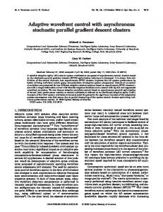
Fig. 1. Microphotographs of micromachined mirror arrays used in the experiments: 共a兲 BUtt segmented membrane tip-tilt mirror with 4 ⫻ 4 elements 共5 ⫻ 5 actuators兲,5 共b兲 MOz piston-type mirror array with zig-zag spring, 共c兲 MOs piston-type mirror array with spiral spring,6 共d兲 BU12 12 ⫻ 12 actuator tip-tilt mirror array, 共e兲 UC piston-type 12 ⫻ 12 mirror array,7,17 共f 兲 OKO continuous-membrane mirror.8 MO and UC mirrors are shown without lenslet arrays. Photographs of magnified mirror elements are shown at the bottom right in 共a兲–共e兲. Mirror array structural elements are marked by capital letters: M, mirror elements; S, spring 共flexure兲; and P, actuator post. Both BUtt and BU12 are made without a metallic reflecting coating and thus the polysilicon membrane surface is partially transparent.

sensors and corresponding microscale phasereconstruction computational hardware. This cannot be easily achieved with existing wave-front sensing techniques. Thus the arrival of highresolution ␮-mirror arrays demands the development of new MEMS-friendly adaptive wave-front control techniques. Among recent adaptive wave-front control algorithms the stochastic parallel gradient descent optimization technique is perhaps the most promising for MEMS-based adaptive optics.11–14 This algorithm does not require wave-front sensing and provides compact, low-power, scalable to high-resolution hardware implementation in a VLSI adaptive controller interfaced 共or potentially integrated兲 with micromachined mirror arrays. Such a VLSI adaptive controller 共e.g., the AdOpt control system15兲 has been developed and used in recent experiments with a 127-element liquid-crystal phase modulator and a 37control-channel continuously deformable micromachined mirror.16 The AdOpt control system architecture is ideal for evaluation of MEMS-based adaptive optics. Because stochastic parallel gradient descent control is model free and independent of ␮-mirror characteristics, different types of micromachined mirror device 4244

APPLIED OPTICS 兾 Vol. 40, No. 24 兾 20 August 2001

can be examined by use of the same adaptive system configuration. The high operational rate of the VLSI controller 共up to 200 kHz兲 well exceeds the dynamic range of all existing ␮ mirrors, which makes the entire adaptation rate dependent only on the dynamic properties of the micromachined mirrors. We begin this paper with an attempt to proceed with MEMS-based adaptive optics through the incorporation of recently developed micromachined mirror arrays and VLSI microelectronic control systems. Here we analyze and compare the performance of what are to our knowledge the first adaptive systems composed only of microscale on-chip elements: ␮-mirror arrays and a VLSI stochastic gradient descent microelectronic control system. 2. Microelectromechanical Mirror Arrays

Photographs of the micromachined mirror arrays used in the experiments described below are shown in Figs. 1共a兲–1共e兲. For adequate comparison of adaptive-system performance we carried out the closed-loop experiments with ␮-mirror arrays that had approximately the same numbers of elements. These mirrors are the 5 ⫻ 5 element tip-tilt control ␮ mirror developed at Boston University 共the BUtt mirror兲 in Fig. 1共a兲 and two types of 6 ⫻ 6 element

piston-only control mirror made by MEMS Optical, Inc. 共the MOz and MOs mirrors兲 shown in Figs. 1共b兲 and 1共c兲. The BUtt mirror in Fig. 1共a兲 is composed of a segmented silicone membrane supported by an underlying array of electrostatic parallel-plate actuators 共posts兲 located at the mirror element corners. The mirror surface contains the print-through pattern that is visible in Fig. 1共a兲. The MOz and MOs mirrors in Figs. 1共b兲 and 1共c兲 have differently shaped springs S holding mirror elements M: zigzag for the MOz and spiral-shaped for the MOs mirrors. We also examined 共in an open-loop system only兲 the characteristics of two 12 ⫻ 12 mirror arrays developed at Boston University 关tip-tilt-type BU12 mirror in Fig. 1共d兲兴 and of one from the University of Colorado at Boulder 关piston-type UC mirror shown in Fig. 1共e兲兴 and a 37-electrode micromachined deformable mirror from OKO Technologies 关Fig. 1共f 兲兴. To increase the fill factor and partially overcome problems related to the optical quality of the mirror surfaces we used all mirror arrays except the BU ␮ mirrors and the OKO mirror with a lenslet array attached to the ␮-mirror chip. The experiments showed that a lenslet array composed of short 共6-mm or less兲 focallength lenses introduces additional phase distortions 共defocus and spherical aberrations兲 that cannot be compensated for by the adaptive system itself. In addition, use of the lenslet array typically provides a fill factor of less than 75% and requires rather precise adjustment, to ensure 90° illumination of the mirror surface. The interference and focal-plane intensity patterns presented in Fig. 2 illustrate the optical quality of the micromachined mirrors in the absence of applied voltages. The elements of the BUtt mirror array in Figs. 2共a兲 and 2共b兲 display the presence of a rather strong unwanted curvature. In the more-recent ␮ mirror 关BU12 mirror in Figs. 2共c兲 and 2共d兲兴 this curvature was almost completely eliminated by ioninduced compression of the mirror surface. The typical interference and focal-plane intensity patterns of the MOs mirror with the lenslet array in Figs. 2共e兲 and 2共f 兲 display the presence of severe wavefront aberrations that result from the optical quality of both the mirror surface and the lenslet array. The MOz mirror with the lenslet array had an optical quality similar to that shown in Figs. 2共e兲 and 2共f 兲. Typically, ␮-mirror electromechanical characteristics are described in terms of voltage-deflection curves 共the dependence of the actuator’s deflection on applied voltage兲.5,18 For analysis of the adaptive system based on performance metric optimization described below, it is more appropriate to use a different characteristic, which we call Strehl ratio sensitivity curves. We estimated the electromechanical characteristics of the ␮-mirror elements by measuring the dependence of Strehl ratio 共St兲 on voltages uj 共 j ⫽ 1, . . . , N兲 applied to various ␮-mirror electrodes 共N is the number of actuators兲. The Strehl ratio is defined as St共uj 兲 ⫽ P共uj 兲兾P0, where P共uj 兲 and P0 ⫽ P共uj ⫽ 0兲 are optical power values measured inside a 50-␮m pinhole placed in the focal plane of a lens with

Fig. 2. 共a兲, 共c兲, 共e兲 Mirror surface interference patterns and 共b兲, 共d兲, 共f 兲 corresponding far-field intensity distributions with no applied voltages for 共a兲, 共b兲 the BUtt mirror, 共c兲, 共d兲 the BU12 mirror, and 共e兲, 共f 兲 the MOs mirror with a diffractive lenslet array 共e, f 兲.

focal length F ⫽ 15 cm 共Fig. 3兲. Results of the Strehl ratio measurements are presented in Fig. 4 for MOs and for BUtt mirror chips for three different actuator locations. For the piston-type MOs mirror the dependencies St共uj 兲 are periodic functions 关Fig. 4共a兲兴 with approximately equal-amplitude maxima that correspond to 2␲ rad phase shifts. As can be seen from Fig. 4共a兲, the mirror stroke depends on the actuator’s location and varies from ⬃1.27 ␮m 共3.75 ␲ phase shift兲 for the corner element to 1.5 ␮m for the actuator located in the mirror center. The Strehl ratio sensitivity curves for the tip-tilt mirror array 共BUtt mirror兲 presented in Fig. 4共b兲 are quite different

Fig. 3. Schematic of the experimental setup for Strehl ratio measurements. 20 August 2001 兾 Vol. 40, No. 24 兾 APPLIED OPTICS

4245

Fig. 5. Strehl ratio resonance curves for the micromachined mirrors examined. Resonance curves for OKO, UC, MOs, and MOz mirrors are shown in linear scales and the BU mirror on a logarithmic frequency scale. Fig. 4. Dependence of Strehl ratio on voltage applied to a single actuator for 共a兲 the MOs and 共b兲 the BUtt mirrors. Strehl ratio sensitivity curves 1, 2, and 3 correspond to three actuator locations within the mirror array, as shown at the bottom left 共M is a mirror element; P is an actuator post兲.

from the corresponding curves for the piston-type mirror 关cf. the curves in Figs. 4共a兲 and 4共b兲兴. These curves are also periodic with 2␲ rad phase shifts between local maxima, but, Fig. 4共b兲 shows, the amplitude of the Strehl ratio local maximum decreases with an increase in the actuator displacement. The dependence of the sensitivity curve on actuator location is more pronounced for the tip-tilt mirror than for the piston-type mirror in Fig. 4共a兲. Spatial nonuniformity in the actuator sensitivity and the presence of local maxima complicates control-system design, especially if the corresponding ␮ mirror is used in a phase-conjugation-type adaptive optical system.19 A technique similar to the one described above was used for evaluation of the ␮-mirror elements’ dynamic characteristics. In the scheme in Fig. 3 a small-amplitude probe voltage u共t兲 ⫽ a sin共␯t兲 ⫹ a0 was applied to a single ␮-mirror actuator, where a and v are the ac component amplitude and frequency, respectively, and a0 is an offset voltage. The measured dependencies of Strehl ratio amplitude St共␯兲 on frequency ␯ 共Strehl ratio resonance curves兲 are shown in Fig. 5 for several ␮-mirror types. The first resonance was observed at frequencies ␯0 ⬵ 2 kHz for the OKO mirror, ␯0 ⬵ 5.3 kHz for the MOs mirror, and ␯0 ⬵ 5.8 kHz for the MOz mirror. For both the BUtt and the UC mirrors the observed dependencies St共␯兲 had no resonance peaks within the examined frequency bands of 100 and 20 kHz, respectively. The BUtt mirror chip displayed relatively uniform dynamic characteristics within a frequency bandwidth of ⬃10 kHz. The major characteristics of the ␮ mirrors that we examined are summarized in Table 1. Based on the previous analysis, the following ␮ mirrors were chosen for closed-loop experiments with the microscale 共MEMS–VLSI兲 adaptive system: the 4246

APPLIED OPTICS 兾 Vol. 40, No. 24 兾 20 August 2001

tip-tilt type 5 ⫻ 5 mirror array from Boston University 共BUtt mirror兲 and two piston-type 6 ⫻ 6 mirror arrays from MEMS Optical, Inc. 共the MOs and MOz mirrors兲. The rationale behind this choice is as follows: The BUtt mirror chip provides the best dynamic operational range among the ␮ mirrors examined, but it cannot be interfaced directly with the AdOpt VLSI controller in its present form, fabricated in a standard complementary metal-oxide semiconductor process. The output control voltages from the VLSI controller chips are within the range of ⫺5 to ⫹5 V. These voltages are not sufficiently high to drive the BUtt mirror array. As can be seen from the sensitivity curves in Fig. 4共b兲, the BUtt mirror requires an ⬃200-V control voltage range to provide a 2␲ phase shift. For this reason amplifiers with output voltages in the range 0 –300 V were used to interface the BUtt mirror with the VLSI controller. The set of 26 amplifiers developed at Boston University was built onto one 6.5⬙ ⫻ 4.5⬙ 共16.51 cm ⫻ 11.43 cm兲 board. The need for external high-voltage amplifiers is highly undesirable for the future development of high-resolution microscale adaptive systems. From this point of view the low-voltage MO and UC mirrors have the obvious advantage 共unless highvoltage amplifiers are integrated onto the MEMS chip兲: both of these mirrors can be interfaced with the VLSI controller directly to form a microscale adaptive system. In the closed-loop experiments with MO mirrors an additional constant 共offset兲 voltage u0 was applied to the mirrors’ common electrode to permit direct interfacing of the VLSI controller with the MOs mirror array. With the offset voltage u0 ⫽ ⫺25 V, the MOs mirror operated with input control voltages that ranged from 20 to 30 V and provided an approximately 4␲ wave-front phase shift 关see the sensitivity curves in Fig. 4共a兲兴. For the MOz mirror an offset voltage of ⫺10 V was sufficient to provide a phase shift near 3.5␲, with the control voltage ranging from 5 to 15 V.

Table 1. Parameters of the ␮-Mirror Chips Used in the Experiments

Mirror

Type of Motion

MOz MOs UC BUtt OKO

Piston Piston Piston Tip-tilt Continuous membrane

Number of Actuators

Mirror Element Size

36 36 128 共36 used兲 25 37

160 ␮m 100 ␮m 74 ␮m 242 ␮m 12-mm active aperture

Actuator Pitch

Actuator Voltage Range 共V兲

Stroke 共␮m兲

Resonance Frequency

500 ␮m 共rectangular兲 500 ␮m 共rectangular兲 250 ␮m 共rectangular兲 250 ␮m 共rectangular兲 1.75 mm 共hexagonal兲

0–15 0–30 0–11 0–300 0–210

0.7 1.1 0.9 0.9 6 共center兲

5.8 kHz 5.3 kHz Not observed Not observed 2 kHz 共1st peak兲

3. Microscale MEMS–VLSI Adaptive System A.

Experimental Setup

A schematic of the microscale VLSI–MEMS-based adaptive system is shown in Fig. 6. Key system elements include a micromachined mirror, a VLSI controller, and a photodetector, as presented in Fig. 7. The expanded input laser beam from the semiconductor laser 共␭ ⫽ 0.69 ␮m兲 with a diameter of ⬃8 mm was split into two equal parts by beam splitter BS1 共Fig. 6兲. Reference mirror M and micromachined mirror ␮–M formed an interferometer that was used to visualize the wave-front phase pattern in the plane of camera CCD1. An imaging system composed of lenses L1 and L2 formed a magnified image of the ␮-mirror surface at the camera chip. The wave reflected from the ␮ mirror was focused by lens L1 and beam splitter BS2 onto the plane of the 50-␮m pinhole. To prevent the reference beam from entering the pinhole we slightly tilted the reference mirror. The laser beam’s power inside the pinhole was measured with a photodetector, and the photodetector’s output voltage was used as the adaptive system’s performance metric 共beam-quality metric兲 J. This beam-quality metric is proportional to the previously defined Strehl ratio St and depends on voltages 兵uj 其 applied to the ␮-mirror electrodes: J ⫽ J共u1, . . . , uN兲, where N ⫽ 25 for BUtt and N ⫽ 36 for MO mirrors. Accordingly, maximization of beamquality metric J is equivalent to Strehl ratio maximization. Lens L3 and beam splitter BS3 were used

Fig. 6. Schematic of the microscale adaptive-optics system based on the AdOpt VLSI controller and micromachined mirrors used in the experiments.

to magnify the image of the laser beam’s intensity distribution in the plane conjugate to the pinhole. This intensity distribution was registered by camera CCD2. Iris diaphragm D placed in the focal plane of lens L1 was used as a low-pass spatial filter to cut off the higher-order spectral components that resulted from laser beam diffraction off the periodic structure of the ␮-mirror array. B.

VLSI Feedback Controller

Adaptive feedback control of the ␮-mirror arrays was achieved with VLSI implementation of the parallel stochastic perturbative gradient descent algorithm 共AdOpt control system architecture兲.15,16 The VLSI controller performed iterative parallel computation 共upgrade兲 of control voltages 兵uj 其 applied to the ␮-mirror electrodes, leading to maximization– minimization of the externally supplied performance metric J. A single AdOpt chip provided parallel updates for 19 output-control signals. Correspondingly, two AdOpt chips were enough to control the micromachined mirror arrays used in the experi-

Fig. 7. Photograph of the key elements 共VLSI controller board, ␮ mirror, and photodetector兲 of the microscale adaptive-optics system based on stochastic parallel gradient descent optimization. The VLSI controller board comprises 7 AdOpt chips and can provide control of as many as 133 channels. The U.S. quarter coin at the bottom right is used to indicate the scale. 20 August 2001 兾 Vol. 40, No. 24 兾 APPLIED OPTICS

4247

Fig. 8. Simplified timing diagrams for a single iteration cycle of the AdOpt system: sequence of external clock signals supplied to the AdOpt chips 共top兲, clock signals used for beam-quality metric measurements 共middle兲, corresponding sequence of changes in beam-quality metric J 共bottom兲.

ments. The VLSI controller requires both analog and digital externally supplied control signals generated by a desktop PC with two analog– digital input– output cards 共ComputerBoards CIO-DAS1602兾12兲. The computer generated the timing signals, controlled measurements of beam-quality metric J, and updated the algorithm parameters. Controlling the VLSI system parameters permitted implementation of a secondary control-loop system designed to modify the algorithm parameters during the adaptation process to increase its convergence rate 共see Subsection 4.D below兲. Using a computer to control the AdOpt system was convenient for analysis of system performance. In actual microscale systems the computer can be replaced by a microcontroller integrated on the AdOpt board. As an illustration of VLSI controller operational principles, consider the simplified timing diagram shown in Fig. 8. A single iteration cycle of the control voltage’s update at the nth iterative step consists of the following phases: 共1兲 A clock signal from the computer board is applied to the VLSI controller digital input at the moment t ⫽ t0. This signal activates on-chip generation of an uncorrelated pseudorandom parallel stream of coin-flip signals 共perturbations兲 兵␦uj共n兲其 that have identical amplitudes 兩␦uj共n兲兩 ⫽ ␲ and a Bernoulli probability distribution P关␦uj共n兲 ⫽ ⫹␲兴 ⫽ 0.5 for all j ⫽ 1, . . . N and all n. These perturbations are applied in parallel to the VLSI system’s output electrodes interfaced directly with the micromachined mirror electrodes 共for MOs and MOz mirrors兲 or through amplifiers 共for the BUtt mirror兲. Voltage perturbations result in a variation in the laser beam power inside the pinhole and hence 4248

APPLIED OPTICS 兾 Vol. 40, No. 24 兾 20 August 2001

in a variation of the photodetector’s output voltage that corresponds to beam-quality metric J. The per共n兲 turbed beam-quality metric value J共n兲 ⫹ ⫹ ⫽ J关u1 共n兲 共n兲 共n兲 ␦u1 , . . . , uN ⫹ ␦uN 兴 is measured at the moment t1 ⫽ t0 ⫹ ␶del after a time delay ␶del introduced by the PC computer. The controllable time delay was introduced to prevent ␮-mirror dynamics from influencing metric measurement: ␶del ⬇ 1.5␶␮, where ␶␮ ⫽ 2␲兾␯0 is the ␮ mirror’s characteristic response time and ␯0 is resonance frequency. 共2兲 When metric value J共n兲 ⫹ has been measured 共at t2 ⫽ t1 ⫹ ␶m, where ␶m ⬵ 45 ␮s兲, the computer board activates on-chip generation of complementary perturbations 兵⫺␦uj共n兲其 at moment t3. These perturbations applied to the ␮-mirror array result in a corresponding change in beam-quality metric J共n兲 ⫺ ⫽ 共n兲 共n兲 J关u1共n兲 ⫺ ␦u1共n兲, . . . , uN ⫺ ␦uN 兴. 共3兲 After the computer introduces time delay ␶del, the perturbed beam-quality metric value J共n兲 ⫺ is measured and digitized. In the timing diagram in Fig. 8 this measurement corresponds to moment t4 ⫽ t3 ⫹ ␶del. After the measurement 共at time t5 ⫽ t4 ⫹ ␶m兲, perturbation voltages are deactivated. 共4兲 Using perturbed beam-quality metric values 共n兲 J共n兲 ⫹ and J⫺ , the computer calculates the following 共n兲 quantities: metric perturbation, ␦J共n兲 ⫽ J共n兲 ⫹ ⫺ J⫺ ; 共n兲 共n兲 共n兲 共n兲 1 averaged metric, J ⫽ ⁄2 关 J⫹ ⫹ J⫺ 兴; sign关␦J 兴; and the product of ␥␦J共n兲, where ␥ is a predefined upgrade coefficient. With a 400-MHz PC the time required for these calculations, ␶cal, is less than 0.1 ␮s. Parameter ␥ controls the update rate and the optimization mode of the performance metric: Positive ␥ corresponds to metric maximization; negative, to metric minimization. The product ␥ ␦J共n兲 is used to generate the update pulse ␶up ⫽ ␥兩␦J共n兲兩⌬tc applied to the VLSI chip input, where ⌬tc is the duration of the clock pulses. In the feedback control system described here, ⌬tc ⬵ 1.0 ␮s. The control-voltage update phase starts at time t6 and lasts a duration of ␶up 共typically ␶up varies from ⌬tc to 25⌬tc兲. During this time the VLSI controller computes updated control-output voltages according to the following gradient descent procedure: u j共n⫹1兲 ⫽ u j共n兲 ⫹ ␥⬘兩␦J 共n兲兩sign关␦J 共n兲兴sign关␦u j共n兲兴,

(1)

where ␥⬘ is a constant that is proportional to ␥. Using the AdOpt system, one can obtain the outputvoltage change for each control channel 关the second term in Eq. 共1兲兴 by charging– discharging a set of on-chip capacitors during the update time ␶up ⫽ ␥兩␦J共n兲兩⌬tc. The value sign关␦J共n兲兴 is supplied to the chip input through the PC board, and the values sign关␦uj共n兲兴 are stored on-chip. With the use of a 1.0-MHz external-clock generator and two analog– digital input– output boards 共ComputerBoards CIO-DAS1602兾12兲, one iteration of the control-voltages update required ␶it ⬇ 160 ␮s 共in the absence of the computer-introduced time delay ␶del兲. Using commercially available fast analog– digital converters, one can further decrease the time required for a single iteration to ␶it ⬇ 100 ␮s.

4. Self-Induced Phase-Distortion Compensation A.

Characterization of Adaptive-System Performance

Adaptive-system performance was characterized by the self-induced aberration-compensation technique described in Refs. 15 and 16. In this method random phase distortions are introduced by an adaptive system as a result of minimization of the beam-quality metric. For statistical analysis of system operation we used a large number M of consecutively repeated adaptation trials 共typically M ⫽ 500兲. Each adaptation trial included a sequence of Nit ⫽ 4096 iteration steps n 共control-voltage updates兲 executed by the AdOpt system 共n ⫽ 1, . . . , Nit兲. During the first 2048 iteration steps the update parameter ␥ set by the computer was negative, which corresponded to minimization of the beam-quality metric. This adaptation mode was used to generate random phase distortions that resulted in a highly distorted laser beam intensity distribution in the plane of the photodetector. At the iteration n ⫽ 共1⁄2Nit ⫹ 1兲 ⫽ 2049 the sign of update parameter ␥, and hence the adaptation mode, was changed. At this second phase of the adaptation trial 共from n ⫽ 2049 to n ⫽ 4096兲 the adaptive system maximized the beam-quality metric such that the laser beam’s power was concentrated inside the pinhole. At each iteration the measured perturbed beam-quality metric values 共n兲 共n兲 J共n兲 J共n兲 ⫽ 关 J共n兲 ⫹ and J⫺ were averaged: ⫹ ⫹ J⫺ 兴兾2. 共n兲 The metric values 兵 J 其 共n ⫽ 1, . . . , 4096兲 as well as the metric perturbation values 兵␦J共n兲其 were stored in computer memory. The complete set of data used for statistical analysis of adaptive-system performance included metric values 兵 J共n兲其 and 兵␦J共n兲其 collected for M consecutively repeated adaptation trials. B.

Convergence Rate and Adaptation Speed

An example of typical dependence of metric J on iteration number n 共adaptation evolution curve兲 obtained during a single minimization–maximization trial is shown in Fig. 9共a兲 for the closed-loop system with the BUtt mirror. Note that the optimization mode 共sign of the update coefficient ␥兲 was changed from metric maximization to minimization at n ⫽ 1 and vice versa at n ⫽ 2049. The iteration number n ⫽ 0 corresponds to the last iteration of the previous trial 共n ⫽ 4096兲. The adaptation evolution curve 具J共n兲典 averaged over all 500 trials is presented in Fig. 9共b兲. From the evolution curve 具J共n兲典 one can estimate an adaptation convergence rate, defined here as the average number of iterations ncmax 共or ncmin兲 required for achieving 80% of the maximum 共minimum兲 level of the beam-quality metric. From the adaptation evolution curve in Fig. 9共b兲, the convergence rate is approximately ncmax ⬇ 60 iterations for metric maximization and ncmin ⬇ 140 iterations for metric minimization. The difference in adaptation rates 共beam-quality metric maximization occurs on average twice as fast as metric minimization兲 is due to two major factors. The first is the decrease in signal-to-noise ratio that occurs during metric minimization, which slows down the adaptation process. The second factor is

Fig. 9. Experimental results of self-induced phase-distortion compensation in an adaptive system with the BUtt mirror: adaptation evolution curves for optimization of the beam-quality metric 共a兲 for a single trial and 共b兲 after averaging over 500 trials. Photographs correspond to focal-plane intensity distributions at the end of minimization 共left兲 and maximization 共right兲. The transition process 共⬃60 iteration long兲 is shown in 共b兲 as an inset.

the existence of a large number of local minima such that the adaptive system may be trapped during the minimization process. This problem is discussed in Subsection 4.C below. The characteristic adaptation time ␶ad is the product of convergence rate ncmax and time ␶it required for a single iteration of control-voltage update 共␶it is dependent on time delay ␶del introduced by the computer兲: ␶ad ⫽ ncmax ␶it. In the experiments with different ␮ mirrors, we used the minimum possible time-delay value ␶del for each mirror that still ensured stable adaptation. This minimal time-delay value depended on the ␮ mirror’s frequency bandwidth. For the fastest 共BUtt兲 mirror this time delay was set to zero. The averaged adaptation evolution curves 具J共t兲典 for the system with BUtt, MOz, and MOs are presented in Fig. 10 as functions of physical time t. The shortest adaptation time ␶ad 共⬇10 ms兲 was achieved with the BUtt mirror array. The limiting factor for the BUtt mirror was not the mirror’s mechanical bandwidth 共⬇10 kHz兲 but the speed of the computer boards. For the MOz and MOs mirrors the adaptation time was limited by mechanical resonance of the mirror actuators, with ␶ad ⬇ 105–120 ms for both MO mirrors 共see the resonance curves in Fig. 5兲. The photos in Fig. 10 show intensity distributions in the focal plane 共plane of the pinhole in Fig. 6兲 obtained in the adaptive system with an MOs mirror array. Metric minimization typically led to the appearance of a dark spot in the pinhole, as shown in Fig. 10 共left photo兲, whereas metric maximization always resulted in laser beam concentration in the pin20 August 2001 兾 Vol. 40, No. 24 兾 APPLIED OPTICS

4249

Fig. 10. Beam-quality metric evolution curves averaged over 500 maximization trials 具J共t兲典 for the following ␮-mirror arrays: BUtt, MOs, and MOz. Photographs show typical snapshots of focalplane intensity distributions for the MOs mirror at 共left兲 t ⫽ 0 and 共right兲 t ⫽ 200 ms.

hole area 关Fig. 10 共right photo兲兴. Note that the estimated adaptation time ␶ad represents the rather pessimistic situation when the adaptive system is compensating for specially prepared temporally uncorrelated random phase distortions that correspond to the most severe wave-front aberrations that can be created with the ␮ mirror. C.

Local Extrema

As one can learn from experiments, the adaptation evolution curves do not always converge to the same stationary state maximum or minimum that displays the presence of local extrema of the beam-quality metric as seen in Fig. 11. The existence of local maxima is perhaps one of the most difficult problems for adaptive wave-front control techniques based on optimization of the system performance metric.14 –16 The following problems should be addressed to re-

Fig. 11. Adaptation evolution curves for beam-quality metric 共a兲 minimization and 共b兲 maximization for a tip-tilt mirror array 共BUtt兲 adaptive system. Curves correspond to four adaptation trials. 4250

APPLIED OPTICS 兾 Vol. 40, No. 24 兾 20 August 2001

veal the potential negative effect of the local extrema on adaptive-system performance: 共1兲 Origin of local extrema and their dependence on type and resolution of the adaptive mirror. 共2兲 Frequency of occurrence 共probability of occurrence兲 of local extrema and the difference 共distance兲 between local and global metric values. The origin of local maxima can be illustrated with the single-element sensitivity curves presented in Fig. 4. Assume that at some moment t all elements– actuators of a ␮ mirror are aligned properly, except a single element 关curve 2 in either Fig. 4共a兲 or 4共b兲兴. The state of this adaptive system corresponds to point A on the sensitivity curve in Fig. 4. Maximization of the beam-quality metric with a gradient ascent technique will result in the system’s transitioning to the state that corresponds to the closest local maximum 共point A⬘ in Fig. 4兲. For a tip-tilt mirror 关Fig. 4共b兲兴 the metric value 共Strehl ratio兲 at the local maximum is significantly less than at the global maximum 共perfectly adjusted system兲. For a piston-type mirror 关Fig. 4共a兲兴 the situation is different. The Strehl ratio at the local maximum has almost the same value as at the global maximum. For a perfect piston-type mirror, not all local maxima are distinguished. This situation corresponds to 2␲-degenerate local maxima that have the same 共optimal兲 Strehl ratio St values. Degeneracy of the local maxima is absent for tip-tilt and continuously deformable surface mirrors. One can decrease the effects of local maxima by increasing the perturbation amplitudes 兵␦uj共n兲其 applied to the mirror electrodes, by increasing update coefficient ␥, or both. In both cases the system has a higher probability of not getting trapped in the vicinity of the small-amplitude local maxima that compose the majority of the total local maxima. The adaptation process rather will converge to the global maximum or to a local maximum that corresponds to a metric value that is only slightly different from the global value. Increasing the perturbation amplitude and the update coefficient, however, may cause such negative effects as unwanted metric oscillation in the vicinity of a maximum. The problem of local maxima can be analyzed by calculation of probability distribution p共 J兲 for beamquality metric J. The transition processes 共from metric maximization to minimization and vice versa兲 may affect the accuracy of the calculated probability distributions. To avoid this effect we estimated probability distribution p共 J兲, using measured values of beam-quality metric J共n兲 for the last 1000 iterations of metric maximization pmax共 J兲 and minimization pmin共 J兲 collected from all 500 adaptation trials: p共 J兲⌬J ⫽ NJ兾N0, where NJ is the number of cases that correspond to the beam-quality metric that belongs to the range J ⱕ J ⬍ J ⫹ ⌬J and N0 is the entire number of stored values of metric J. The minimal metric interval used for data collection corresponded to ⌬J ⫽ Jmax兾400 共 Jmax ⫽ max J兲. Probability curves for the beam-quality metric maximization and minimization in Fig. 12共a兲 display the presence of local extrema only for the adaptive system with the

Fig. 12. Probability-density distributions of beam-quality metrics pmax and pmin obtained during 500 adaptation trials: 共a兲 adaptive system with the MOs and BUtt ␮ mirrors and fixed update coefficient ␥ ⫽ 60 and 共b兲 probability distribution pmax for the adaptive system with the BUtt ␮ mirror for three values of the update coefficient ␥. Beam-quality metric J is normalized by its maximum value Jmax.

tip-tilt type BUtt mirror. The probabilities for these local extrema are relatively small. As expected, the probability distributions for the adaptive system with the piston-type MOs mirror are unimodal: All local extrema are 2␲ degenerate and have approximately the same metric values. In the case of the tip-tilttype BUtt mirror, increasing the update coefficient value ␥ eliminated local states in the adaptive system’s dynamics but at the expense of widening the probability-density curves because of the increase in metric oscillations that occurs in the vicinity of the global maximum, as shown in Fig. 12共b兲. D. Control of Adaptation Rate: Coefficient through Learning

Change in Update

As we mentioned in Subsection 3.B, the system’s adaptation rate depends on the value of update coefficient ␥ that is externally supplied to the VLSI chips. Thus the AdOpt control system architecture permits on-the-fly 共at each iteration兲 control of the update coefficient. For control of coefficient ␥ the following information was available: the perturbed beam共n兲 quality metric values J共n兲 ⫹ and J⫺ measured at each iteration and the calculated difference 共metric per共n兲 turbation兲 ␦J共n兲 ⫽ J共n兲 In the experiments ⫹ ⫺ J⫺ . described below we also performed at each iteration an additional measurement of the unperturbed metric value J共n兲 and calculated two additional metric 共n兲 共n兲 共n兲 perturbations: ⌬J共n兲 and ⌬J共n兲 ⫹ ⫽ J⫹ ⫺ J ⫺ ⫽ J⫺ ⫺ 共n兲 共n兲 J . The measurement of J lasted ⬃25 ␮s. In the absence of the introduced time delay ␶del this additional measurement resulted in a nearly 15% increase in the time ␶it required for a single iteration. A portion of the obtained data was saved in computer memory, thus permitting the use of data from previous l ⫽ 1, . . . , L iterations 共control with L-step-long

Fig. 13. Convergence rate ncmax of the adaptation process relative to update coefficient ␥ for maximization of the beam-quality metric in an adaptive system with the BUtt mirror. The metric fluctuation level is characterized by the normalized standard-deviation values ␴៮ J shown in parentheses. The diamond represents results obtained in the system with a change in the adaptive update coefficient. The fluctuation level in the system without adaptation was near 0.01.

memory兲. With a 400-MHz PC computer the additional time required for the calculations and data storage was less then 1.5 ␮s and can be neglected. The question is how to use this available information to control the update coefficient. First, consider the dependence of the adaptation process’s convergence rate ncmax 共number of iterations required to reach 80% of the beam-quality metric’s maximum value兲 on the update coefficient ␥ as presented in Fig. 13. As expected, an increase in ␥ resulted in acceleration of the convergence speed of the adaptation 共ncmax decrease兲. However, decreasing ncmax increased the normalized standard deviation of beam-quality metric fluctuations, defined as 4096 ␴៮ J ⫽ 0.001 ¥n⫽3097 兵具关共 J共n兲 ⫺ 具J共n兲典兴2典1兾2兾具J共n兲典其. Standard deviation ␴៮ J included averaging over the last 1000 iterations of each optimization trial. The values ␴៮ J obtained in the experiment are shown in parentheses in Fig. 13. Increasing ␥ is advantageous only during the transition phase of the adaptation process and is unfavorable when the adaptive system is near the extremum. It follows that adaptive control should provide for an automatic increase in the update coefficient during the transition phase and for a decrease otherwise. The problem is to determine the current phase of the adaptation process 共transition, near minimum, near maximum兲 and use this information for iterative change of the upgrade coefficient. We used the following three quantities 共indicators兲 H共n兲 to identify phase in the adaptation process: 共n兲 共n兲 H 1共n兲 ⫽ 兩sign关⌬J ⫹ 兴 ⫺ sign关⌬J ⫺ 兴兩,

H 2共n兲 ⫽ 兩␦J 共n兲兩, L

H 3共n兲 ⫽

兺 兩J

共n兲

⫺ J 共n⫺l 兲兩.

(2)

l⫽1

20 August 2001 兾 Vol. 40, No. 24 兾 APPLIED OPTICS

4251

It is easy to see that at the transition phase all H共n兲 indicators have higher values 共on average兲 than the corresponding values for adaptive-system operation near an extremum. The length of memory L in Eqs. 共2兲 should be less than the typical convergence rate ncmax of the adaptation process. In the experiments we used L ⫽ 5. To decrease the influence of noise we averaged the quantities in Eqs. 共2兲 over a few iterations M1 ⫽ 5: ៮ i共n兲 ⫽ H

1 M1

M1

兺H

共n⫺m兲 i

,

i ⫽ 1, 2, 3.

(3)

m⫽0

For a better understanding of the iterative algorithm used for update coefficient control, consider its continuous-time analog: ␶

d␥ ៮ 共t兲, ⫽ 共␥ 0 ⫺ ␥兲 ⫹ ε 0H dt

(4)

៮ 共t兲 ⫽ H ៮ 1共t兲H ៮ 2共t兲H ៮ 3共t兲 and ␶, ␥0, and ε0 are where H constants 共algorithm parameters兲. In Eq. 共4兲, continuous time t is used instead of iteration number n. ៮ 共t兲 is the product of all The introduced function H three indicators defined in Eq. 共3兲. For adaptivesystem operation near an extremum 共maximum or ៮ 1 vanishes because in the minimum兲 the function H 共n兲 absence of noise the perturbations ⌬J共n兲 ⫹ and ⌬J⫺ have the same sign and their difference 共the function ៮ 1 depends兲 is zero. Correspondingly, upon which H date coefficient ␥ in Eq. 共4兲 approaches the constant value ␥0. At the transition phase the indicator func៮ 共t兲 is positive and increases with increase of the tion H transition process slope. In the accordance with Eq. 共4兲 this procedure creates an increase in update coefficient ␥. The dynamic process of Eq. 共4兲 represents a kind of learning rule that is reminiscent of continuous-type equations in neural network models for changes in weight coefficient through learning 共called long-term memory traces兲.20 The following discrete analog of control algorithm 共5兲 was used in the experiments to control the update coefficient during the adaptation process: ៮ 1共n兲H ៮ 2共n兲H ៮ 3共n兲, ␥ 共n⫹1兲 ⫽ ␥ 共n兲 ⫹ ␣关␥ 0 ⫺ ␥ 共n兲兴 ⫹ εH

(5)

where ␣ and ε are coefficients 共in the experiments we used ␥0 ⫽ 180, ␣ ⫽ 0.9, and ε ⫽ 1500兲. Results of the adaptation with the adaptive-update coefficient change through learning are shown in Fig. 14. The averaged adaptation evolution curve 具J共t兲典 for the system with the BUtt mirror is compared in Fig. 14共a兲 with the evolution curve that corresponds to constant update coefficient ␥ ⫽ ␥0. The dynamics of the update coefficient 具␥共t兲典 averaged over all adaptation trials are shown in Fig. 14共b兲. During the transition stage, ␥ increased ⬃5.8 times compared with the initial value ␥0. One can estimate the gain in the convergence speed of the adaptation process by comparing the characteristic adaptation times ␶ad 共␥兲 and ␶ad shown in Fig. 14共a兲 for the system with con共␥兲 stant 共␶ad兲 and adaptive ␥ 关␶ad 兴 times. The measured 共␥兲 ratio ␶ad兾␶ad indicates a 1.5 increase in the adaptation 4252

APPLIED OPTICS 兾 Vol. 40, No. 24 兾 20 August 2001

Fig. 14. Adaptive system with a change in the adaptive update parameter through learning rule 共4兲: 共a兲 beam-quality metric evolution curve averaged over 1000 trials and 共b兲 corresponding evolution curve for update coefficient ␥. The value ␥0 ⫽ 180 was used in the experiments, with fixed ␥.

speed. The convergence rate that corresponds to the system with adaptive ␥ is labeled with a diamond in Fig. 13. As the related number in parentheses in Fig. 13 indicates, improvement in the convergence rate was obtained without an increase of the metric scintillation amplitude. 5. Conclusion

We have demonstrated microscale adaptive-optics systems formed by combining recently developed micromachined mirror arrays with a VLSI stochastic parallel gradient descent controller. A record adaptation rate of 6000 iterations兾s was achieved with the Boston University mirror array. This system required the use of external amplifiers. We also demonstrated a microscale adaptive system by directly interfacing the low-voltage ␮-mirror array from MEMS Optical, Inc., with the VLSI controller. The adaptive systems considered here with both tip-tiltand piston-type micromachined mirrors arrays have demonstrated efficient compensation for self-induced wave-front phase distortions. The MEMS–VLSI-based wave-front control technique presented here has several attractive features, as follows: 共1兲 Adaptive optics based on the model-free optimization wave-front control technique do not require either a wave-front sensor or computationally expensive wave-front reconstruction hardware. Thus the development of compact, low-power, and inexpensive adaptive systems composed solely of microscale components is facilitated. In this respect the further development of lower-voltage ␮-mirror arrays directly driven by a VLSI controller as well as the integration of high-voltage amplifiers onto a ␮-mirror

chip are important directions for further research for microscale adaptive optics. 共2兲 Micromachined mirror arrays with multikilohertz operational bandwidths are capable of performing tens of thousands of iterations per second. This is exactly what iteration-hungry, modelfree optimization-based adaptive optics needs for compensation of quickly changing atmosphericturbulence-induced wave-front aberrations. As we have demonstrated, the convergence rate of the adaptation process can also be increased by incorporation of an additional long-term memory learning feedback loop. 共3兲 Both the micromachined mirror arrays and the VLSI stochastic gradient descent controller are scalable microscale components that facilitate the development of high-resolution adaptive systems with thousands of wave-front phase-control channels. A potential obstacle to this development is the so-called wiring problem. The ability to control mirror elements in parallel is the major advantage of the stochastic gradient optimization technique and should be preserved during a transition to high-resolution adaptive systems. Possible solutions of the wiring problem are on-chip integration of the VLSI controller with ␮-mirror arrays and flip-chip bonding of ␮-mirror and VLSI controller chips. The authors thank Victor Bright, who generously offered the ␮-mirror array designed at the University of Colorado for examination in our experiments, Gary Carhart for assisting with the computer code, and Jennifer Ricklin for technical and editorial comments. This research was performed at the U.S. Army Research Laboratory’s Intelligent Optics Lab. Research was supported in part through the following U.S. Army and U.S. Air Force programs: Cooperative Agreement DAAD17-99-2-0070 between the U.S. Army Research Laboratory and the Boston University Photonic Center; grant DAAG55-97-1-0114 through the U.S. Army Research Office under the ODDR&E MURI97 program to the Center for Dynamics and Control of Smart Structures 共through Harvard University兲; U.S. Air Force Office of Scientific Research contract F49620-99-1-0342 with New Mexico State University; and U.S. Army Research Office Small Business Innovative Research grant A98-021 to MEMS Optical, Inc. T. Weyrauch currently holds a National Research Council Research Associateship Award at the U.S. Army Research Laboratory.

5.

6.

7.

8.

9.

10.

11.

12.

13.

14.

15.

16.

17.

References 1. N. Maluf, An Introduction to Microelectromechanical Systems Engineering 共Artech House, Norwood, Mass., 2000兲. 2. M. C. Wu, “Micromachining for optical and optoelectronic systems,” Proc. IEEE 85, 1833–1856 共1997兲. 3. R. L. Clark, J. R. Karpinisky, J. A. Hammer, R. B. Anderson, R. L. Lindsey, D. M. Brown, and P. H. Merritt, “Micro-optoelectro-mechanical 共MOEM兲 adaptive optic system,” in Miniaturized Systems with Micro-Optics and Micromechanics II, M. E. Motamedi, L. J. Hornbeck, and K. S. Pister, eds., Proc. SPIE 3008, 12–24 共1997兲. 4. T. G. Bifano, R. Krishnamoorthy Mali, J. K. Dorton, J. Per-

18.

19.

20.

reault, N. Vandelli, M. N. Horenstein, and D. A. Castan˜on, “Continuous-membrane surface-micromachined silicon deformable mirror,” Opt. Eng. 36, 1354 –1360 共1997兲. T. G. Bifano, J. Perrault, R. Krishnamoorthy Mali, and M. N. Horenstein, “Microelectromechanical deformable mirrors,” IEEE J. Sel. Top. Quantum Electron. 5, 83– 89 共1999兲. J. A. Hammer, J. Karpinsky, R. L. Clark, and R. Lindsey, “Micro mirrors in adaptive optics systems,” in Proceedings of the World Automation Congress 共WAC ’98兲, M. Jamshidi and C. W. de Silva, eds., Vol. 6 of TSI Press Series 共TSI, Albuquerque, N.M., 1998兲, pp. 575–581. M. K. Lee, W. D. Cowan, B. M. Welsh, V. M. Bright, and M. C. Roggemann, “Aberration-correction results from a segmented microelectromechanical deformable mirror and refractive lenslet array,” Opt. Lett. 23, 645– 647 共1998兲. G. Vdovin, S. Middelhoek, and P. M. Sarro, “Technology and applications of micromachined silicon adaptive mirrors,” Opt. Eng. 36, 1382–1390 共1997兲. J. H. Comtois, V. M. Bright, S. C. Gustafson, and M. A. Michalicek, “Implementation of hexagonal micromirror arrays as phase-mostly spatial light modulator,” in Microelectronic Structures and Microelectromechanical Devices for Optical Processing and Multimedia Applications, W. Bailey, M. E. Motamedi, and F.-C. Luo, eds., Proc. SPIE 2641, 76 – 87 共1995兲. J. Mansell and R. L. Byer, “Micromachined silicon deformable mirror,” in Adaptive Optical System Technologies, D. Bonaccini and R. K. Tyson, eds., Proc. SPIE 3353, 896 –901 共1998兲. J. C. Spall, “A stochastic approximation technique for generating maximum likelihood parameter estimates,” in Proceedings of the American Control Conference 共Institute of Electrical and Electronics Engineers, Piscataway, N.J., 1987兲, pp. 1161–1167. G. Cauwenberghs, “A fast stochastic error-descent algorithm for supervised learning and optimization,” in Advances in Neural Information Processing Systems, S. J. Hanson, J. D. Cowan, and C. L. Giles, eds. 共Morgan Kaufman, San Mateo, Calif., 1993兲, Vol. 5, pp. 244 –251. M. A. Vorontsov, G. W. Carhart, and J. C. Ricklin, “Adaptive phase-distortion correction based on parallel gradient-descent optimization,” Opt. Lett. 22, 907–909 共1997兲. M. A. Vorontsov and V. P. Sivokon, “Stochastic parallel gradient descent technique for high-resolution wave-front phase distortion correction,” J. Opt. Soc. Am. A 15, 2745–2758 共1998兲. R. T. Edwards, M. Cohen, G. Cauwenberghs, M. A. Vorontsov, and G. W. Carhart, “Analog VLSI parallel stochastic optimization for adaptive optics,” in Learning on Silicon, G. Cauwenberghs and M. A. Bazoumi, eds. 共Kluwer Academic, Boston, Mass., 1999兲, pp. 359 –382. M. A. Vorontsov, G. W. Carhart, M. Cohen, and G. Cauwenberghs, “Adaptive optics based on analog parallel stochastic optimization: analysis and experimental demonstration,” J. Opt. Soc. Am. A 17, 1440 –1453 共2000兲. A. Tuantranont, V. M. Bright, W. Zhang, and Y. C. Lee, “Flip chip integration of lenslet arrays on segmented deformable micromirrors,” in Design, Test, and Microfabrication of MEMS and MOEMS, B. Courtois, S. B. Crary, W. Ehrfeld, H. Fujita, J.-M. Karam, and K. W. Markus, eds., Proc. SPIE 3680, 668 – 678 共1999兲. M. C. Roggeman, V. M. Bright, B. M. Welsh, S. R. Hick, P. C. Roberts, W. D. Cowan, and J. H. Comtois, “Use of microelectro-mechanical deformable mirrors to control aberrations in optical systems: theoretical and experimental results,” Opt. Eng. 36, 1326 –1338 共1997兲. L. Zhu, P.-C. Sun, D.-U. Bartsch, W. R. Freeman, and Y. Fainman, “Adaptive control of a micromachined continuousmembrane deformable mirror for aberration compensation,” Appl. Opt. 38, 168 –176 共1999兲. S. Grossberg, “Nonlinear neural networks: principles, mechanisms, and architectures,” Neural Networks 1, 17– 61 共1988兲.

20 August 2001 兾 Vol. 40, No. 24 兾 APPLIED OPTICS

4253