(time units1). P. (!) (distance units. 2. ) = 1. = 3. = 10. = 30. = 100. 106. 1. 1. 1012 a b c d. Figure 1: Brownian motion results of [1] numerically reproduced from the.
arXiv:chao-dyn/9904041v2 6 Sep 1999
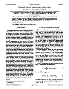
Microscopic chaos from Brownian motion? In a recent Letter in Nature, Gaspard et al. [1] claimed to present empirical evidence for microscopic chaos on a molecular scale from an ingenious experiment using a time series of the positions of a Brownian particle in a liquid. The Letter was preceded by a lead article [2] emphasising the fundamental nature of the experiment. In this note we demonstrate that virtually identical results can be obtained by analysing a corresponding numerical time series of a particle in a manifestly microscopically nonchaotic system. As in Ref. [1] we analyse the position of a single particle colliding with many others. We use the Ehrenfest wind-tree model [3] where the pointlike (“wind”) particle moves in a plane colliding with randomly placed fixed square scatterers (“trees”, Fig. 1a). We choose this model because collisions with the flat sides of the squares do not lead to exponential separation of corresponding points on initially nearby trajectories. This means there are no positive Lyapunov exponents which are characteristic of microscopic chaos here. In contrast the Lorentz model used in [1] as an example similar to Brownian motion is a wind-tree model where the squares are replaced by hard (circular) disks (cf.[1], Fig. 1) and exhibits exponential separation of nearby trajectories, leading to a positive Lyapunov exponent and hence microscopic chaos. Nevertheless, we now demonstrate that the nonchaotic Ehrenfest model reproduces all the results of Ref. [1]. A particle trajectory segment shown in Fig. 1b is strikingly similar to that for the Brownian particle, (cf.[1], Fig. 2). Our subsequent analysis parallels that of Ref. [1], where more details may be found. Thus the microscopic chaoticity is determined by estimating the Kolmogorov-Sinai entropy hKS , using the method of Procaccia and others [4, 5] via the information entropy K(n, ǫ, τ ) obtained from the frequency with which the partical retraces part of its (previous) trajectory within a distance ǫ for n measurements spaced at a time interval τ . Since for the systems considered here hKS equals the sum of the positive Lyapunov exponents, the determination of a positive hKS would imply microscopic chaos. As in [1] we find that K grows linearly with time (Fig 1c and [1] Fig. 3), giving a positive (non-zero) bound on hKS (Fig 1d and [1] Fig. 4). Indeed our Figs. 1b-d for a microscopically nonchaotic model are virtually identical with the corresponding figures 2-4 of [1]. Therefore Gaspard et al. did not prove microscopic chaos for Brownian motion. The algorithm of [4, 5] as applied here cannot determine the microscopic 1
chaoticity of Brownian motion since the time interval between measurements, 1/60 s in [1], is so much larger than the microscopic time scale determined by the inverse collision frequency in a liquid, approximately 10−12 s. A decisive determination of microscopic chaos would involve, it seems at the very least, a time interval τ of the same order as characteristic microscopic time scales. C. P. Dettmann, E. G. D. Cohen Center for Studies in Physics and Biology, Rockefeller University, New York, NY 10021, USA H. van Beijeren Institute for Theoretical Physics, University of Utrecht, 3584 CC Utrecht, The Netherlands
References [1] Gaspard, P. et al Nature 394, 865-868 (1998). [2] Durr, D. & Spohn, H. Nature 394, 831-833 (1998). [3] Ehrenfest, P. & T. The conceptual foundations of the statistical approach in mechanics. (trans. Moravcsik, M. J.) 10-13 (Cornell University Press, Ithaca NY, 1959). [4] Grassberger, P. & Procaccia, I. Phys. Rev. A 28, 2591-2593 (1983). [5] Cohen, A. & Procaccia, I. Phys. Rev. A 31, 1872-1882 (1985).
2000
b
1012
(distance units2 )
a
(distance units)
1950
C
P (! )
y
1900
1
10 6
!
(time units 1 )
1
x
1850
1800
1750 0
x 4
10
( ) (digits per time unit)
c
) (digits)
3
2.5
2
h �; �
(
4000
6000
t
3.5
K n; �; �
2000
1.5
8000
10000
(time units)
d
12000
� � � � �
1
= = = = =
14000
1 3 10 30 100
0.1
0.01
0.001
0.0001 1 1e-05
0.5
0 0
20
40
n�
60
(time units)
80
100
1e-06 0.1
1
10
�
100
(distance units)
Figure 1: Brownian motion results of [1] numerically reproduced from the nonchaotic Ehrenfest wind-tree model (notation as in [1]). The square scatterers have a diagonal of 2 length units and fill half the area considered. The particle moves with unit velocity in four possible directions. The position on its trajectory is determined for 106 points separated by one time unit. (a) Two nearby trajectories split only at a corner C; no exponential separation occurs (cf [1], Fig. 1). (b) A typical trajectory is diffusive, with an ω −2 power spectrum (inset), cf [1], Fig. 2. (c) The information entropy K(n, ǫ, τ ) for τ = 1 and ǫ = 0.316 × 1.21m with m = 0 . . . 25, cf [1], Fig. 3. (d) The envelope of the slopes of these K-curves, h(ǫ, τ ) appears to imply a positive, ie. chaotic, hKS for the Ehrenfest model, as for Brownian motion (cf. [1], Fig. 4).
1000