Microsoft Office Excel 2010 Class 3: Formatting and Printing Page 1 ...

Microsoft Office Excel 2010

Class 3: Formatting and Printing

Home Ribbon: Formatting Tools Dialog Box Launcher: Click this symbol to open old-style dialog box giving additional options

Allow text to appear on multiple lines in a cell

Font controls:  Font, Font Size, Grow Font, Shrink Font  Bold, Italic, Underline, Border, Fill Color, Font Color

Number Format box: Click here Apply any of several shaded color schemes based on the to choose between number document’s Theme colors formats.

Adjust horizontal and vertical alignment of text in cells

Combine several cells into one large cell and center its contents

Change number of decimal places shown Turn comma separator on/off Display numbers as percentages Choose currency symbol

Clear Button Click the dropdown arrow to clear a cell of formats, or of contents, or both

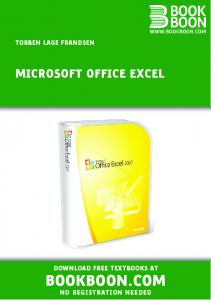
Change the way numbers are displayed (change number formats) Select the cells, rows or columns you wish to affect, then click the dropdown arrow beside the Number Format box in the Number group on the Home Ribbon. The list at right will appear. 

General: All cells have this format by default. Numbers display as typed except that leading and trailing zeroes are deleted. 012.3040 becomes 12.304



Number: Rounds displayed number to two decimal places. 012.3040 becomes 12.30. Rounded number is display only; the real number is still used in math. (multiplying the formatted 12.30 by 1000 comes out 12304)



Currency and Accounting: Round number to two decimal places, add dollar sign and thousands separator. 01457.3040 becomes $1,457.30. Currency format puts the dollar sign next to the number; Accounting format puts it at the left side of the cell.



Short and Long Date: Display numbers as dates. Long Date includes weekday and month in longhand.



Text: Numbers are treated as text characters, not able to be used in math. Can display numbers with more than 15 digits.



More Number Formats button opens a dialog box giving many more options.

Page 1 of 9

Microsoft Office Excel 2010

Class 3: Formatting and Printing

Clear formats from cells Select the cells, rows or columns you wish to affect, then click the Clear button in the Editing group on the Home Ribbon. Choose Clear Formats from the dropdown list. The contents of the cells will be retained, but all formats will be removed and they will go back to the “General” format. Choosing Clear All deletes the contents of the cells as well as removing the formats; choosing Clear Contents removes anything typed in the cells but leaves the formats in place. Fuse several cells into one large cell (merge cells) and split them apart again 1. Select the cells you want to merge into a single large cell. 2. Click the dropdown arrow beside the Merge and Center button in the Alignment group on the Home Ribbon. Choose one of the following: a. Merge and Center: The cells will become one large cell and the text in the cell will be centered. If there is text in more than one cell that is being merged, only the text in the upper left hand cell will be retained. b. Merge Across: Each row’s worth of cells will be merged into a single cell. This lets you select a set of headings and merge each into its own row. c. Merge Cells: Exactly like Merge and Center except that the text will not be centered; it will retain its original alignment. d. Unmerge Cells: Splits a merged cell back into its component cells. Allow text to be on more than one line in a cell (wrap text) 



Select the cells, rows, or columns you wish to affect, then click the Wrap Text button in the Alignment group on the Home Ribbon. These cells will now expand to be tall enough to contain whatever text is typed in them. To remove this effect, click the Wrap Text button again.

Place text into cells at an angle 1. Select the cells, rows, or columns you wish to affect. 2. Click the Orientation button in the Alignment group on the Home Ribbon. 3. Choose the desired text orientation from the drop-down list

Place borders around a group of cells Select a group of cells, then click the Borders button (

) in the Font group on the Home Ribbon.

Choose particular borders from the drop-down list or choose More Borders at the bottom of the list to open the Format Cells dialog box at the Borders tab.

Page 2 of 9

Microsoft Office Excel 2010

Class 3: Formatting and Printing

Change colors of text (Font Color) or cell background (Fill Color)  

  

Select the cells, rows, or columns you wish to affect. The buttons controlling color are located in the Font group of the Home Ribbon. This button: controls fill or background color; this one: controls font or text color. Clicking the dropdown arrow beside either button displays a palette of shaded colors called Theme Colors (see right), with a selection of Standard Colors below. Click the More Colors button to open a palette of all possible colors. Choose a different set of Theme Colors by clicking the Colors button in the Themes group on the Page Layout Ribbon

Quickly apply multiple formats to a data table Select the area to format, and then click Format as Table in the Styles group on the Home Ribbon. Choose the desired table format from the list.  

The table formats are based on the main color and accent colors from your chosen Theme. If you change color themes the table is automatically recolored.

The Table Tools Design Ribbon (contextual ribbon) appears when you are working in a Table. Use it to   

Change shading options (banded rows and columns) Add totals rows Define formats for particular rows or columns.

Cells formatted as Tables also have certain database-like properties. To turn these off, click the Convert to Range button in the Tools group on the Table Tools Design Ribbon. Your colors and formats will be retained and the “database” features will be removed.

Page 3 of 9

Microsoft Office Excel 2010

Class 3: Formatting and Printing

Preview and Print a spreadsheet (Backstage View) View the sheet you want to print. Click the green File tab to enter Backstage View, then click Print in the sidebar at the left. You will see a preview of your document as it would appear when printed.

From this view, you can 

      

Use the navigation control at the bottom to preview each page of your printout. Click the right arrow button () to move to the next page, and the left arrow button () to move to the previous page. Set the number of copies to print. Use the Printer button to choose among your available printers. Use the Print Active Sheets control to set the page range to print. To print only page 2 of a document, for example, type the number 2 in both Pages boxes. Choose single-sided or duplex printing. Choose to collate (print multi-page documents in sets) or not (print all the Page 1s, then all the page 2s and so on). Change page layout options like paper orientation, paper size, margins and scaling. Click the large Print button in the upper left hand corner to send your job to the printer.

Page 4 of 9

Microsoft Office Excel 2010

Class 3: Formatting and Printing

Page Layout Ribbon Select an image to display as the background of the sheet (background image does not print.)

Specify rows and columns to print on every page Shrink width or height of printout to fit a maximum number of pages.

Insert, remove, or reset page breaks

Apply sets of fonts, colors and effects to change the overall look of the document

Switch between Portrait and Landscape orientation

Print lines around cells

Choose from standard margins or specify custom ones.

Tools for arranging graphical objects (Clip Art, Shapes, etc.)

Print row numbers and column letters

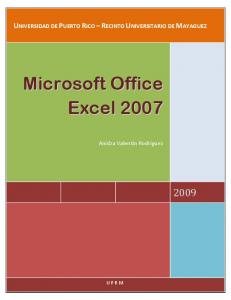
Set margins, center printouts On the Page Layout Ribbon, click the Margins button in the Page Setup group. Choose from the list of common page margins or click Custom Margins to define your own. When you click Custom Margins, the dialog box also displays controls for centering your printout vertically and/or horizontally on the page. Change page orientation On the Page Layout Ribbon, click the Orientation button in the Page Setup group. Click to choose either Portrait (the “tall” way) or Landscape (the “wide” way) orientation. Fit printout onto a specified number of pages On the Page Layout Ribbon, locate the Scale to Fit group. To squeeze all your columns onto one page in the printout, choose One Page under Width and leave Length set to Automatic. In the Scaling box below, you will see the percentage by which Excel is shrinking the spreadsheet’s text. Print row and/or column labels on every page On the Page Layout Ribbon, click the Print Titles button in the Page Setup group. The Page Setup dialog box will open to the Sheet tab:

Page 5 of 9

Microsoft Office Excel 2010

Class 3: Formatting and Printing

Click in the box marked “Rows to repeat at top” under the heading “Print Titles”, and then click the row you want to display on the spreadsheet behind the box. You can also type the numbers for the rows containing the labels. (Ex: If rows 1 and 2 contain the labels, type 1:2 in the box. To print only row 1 at the top of each page, type 1:1 in the box.) For columns, do the same thing using the box marked “Columns to repeat at left”. Print gridlines, row numbers, and/or column letters On the Page Layout Ribbon, locate the Sheet Options group. The two sections are labeled Gridlines and Headings. By default the View button is checked and the Print button is unchecked. Clicking the print box under Gridlines prints lines around each cell even if you have not added borders. Clicking the Print box under Headings prints the row numbers (1, 2, 3…) down the side and the column letters (A, B, C) across the top. View Ribbon

View spreadsheet as it will look when printed; add and edit headers and footers

Make page breaks visible; reposition them by dragging

Work with page breaks To add new page breaks: 1. In column A, click the first cell that you want to appear on the new page. 2. On the Page Layout Ribbon, click the Breaks button in the Page Setup group and choose Insert Page Break. The new page break will appear above the selected cell. To remove page breaks: 1. Click a cell below or to the right of the page break you want to remove. 2. On the Page Layout Ribbon, click the Breaks button in the Page Setup group and choose Remove Page Break. The page break touching the active cell will be removed. To move page breaks: 

 

Click the View tab and click Page Break Preview in the Workbook Views group on the View Ribbon. In this view, solid blue lines mark the end of the region that will print, and dashed blue lines represent Excel’s automatic internal page breaks. Drag the lines with the mouse to adjust the location of your page breaks. Reset all page breaks to their default positions by clicking the Breaks button in the Page Setup group on the Page Layout Ribbon, and choosing Reset All Page Breaks.

Page 6 of 9

Microsoft Office Excel 2010

Class 3: Formatting and Printing

Print headers or footers on every page Anything placed in a header or footer will appear on every page of the printed document.  

 

On the View Ribbon, click the Page Layout button. In Page Layout view the page margins are displayed around the spreadsheet cells. Click in the top or bottom margins where the words “Click to add header” or “Click to add footer” appear. The Header and Footer Design Ribbon will be displayed:

Choose a standard header or footer by clicking the Header or Footer button in the Header & Footer group. Create a custom header or footer by using the Ribbon buttons: o The header and footer areas are divided into a left section, a middle section, and a right section. Click in the desired section to add an element. o Click any button in the Header & Footer Elements group to add that element to the desired section, or type in your own descriptive text. o Click the Go to Header or Go to Footer button in the Navigation group to switch between them. o Create different headers for different parts of the document using buttons in the Options group. Scroll through your document and click in the header section to edit the various headers.

Page 7 of 9

Microsoft Office Excel 2010

Class 3: Formatting and Printing

Practice Exercises 1. Type a spreadsheet with the data below, then do the following: Largest Ohio Libraries (1994) Library Registered Borrowers Akron-Summit County Public Library 198871 Cleveland Public Library 338629 Columbus Metropolitan Library 390970 Cuyahoga County Public Library 468532 Dayton/Montgomery County Public Library 401003 Middletown Public Library 101463 Public Library of Cincinnati and Hamilton County 390334 Public Library of Youngstown and Mahoning County 101484 Stark County District Library, Canton 172513 Toledo-Lucas County Public Library 236193 a. Adjust column size to fit your data. b. Center the table heading (Largest Ohio Libraries (1994)) by merging cells. c. Sort the list into descending order of number of borrowers. (Which library has the most borrowers?) d. Make the column header row bold-faced. e. Change all text to Verdana or Arial Black font. f. Format the numbers to use comma separators and no decimal places.

Page 8 of 9

g. Put dotted lines above/below each row of the table. h. Put solid lines above and below the header row. i. Make the background of the header row a dark color from your theme; make the text a light color. j. Make the background of the rest of the table a light color.

Microsoft Office Excel 2010

Class 3: Formatting and Printing

2. On a fresh sheet, type the following data, starting in cell A1: City First Quarter Ticket Sales Detroit Miami Phoenix Reno

Month 1 Month 2 Month 3 January February March 17 21 36 119 101 89 75 77 61 93 87 90

Second Quarter Ticket Sales April Detroit Miami Phoenix Reno

May 25 240 25 60

June 20 75 185 80

20 360 45 325

a. Use Merge and Center to center the phrase “First Quarter Ticket Sales” over the first quarter data. Do the same for the phrase “Second Quarter Ticket Sales”. b. Use Format As Table to format each quarter’s worth of data. Use two different styles of shading and coloring. c. Set up a header showing the file name and page number. d. Use Page Setup to ensure that Row 1 prints on all pages. e. Insert a page break so that the two quarters’ worth of sales print on two separate pages. f. Either print your work or view it in Print Preview to check that it is correct.

3. Open the ongoing Household Budget project. a. Format your budget’s dollar amounts as currency (use either the Currency or the Accounting format as you prefer.) Readjust the column widths if necessary. b. Fit it to print on one sheet of paper, in the Landscape orientation. c. Adjust the width of your columns to fit the numbers better, using Wrap Text or Orientation to display your column headers in the narrower columns. d. Use Format as Table to add borders and color shading to your budget, and then use Convert to Range to restore the table to “ordinary behavior” (see Page 3). e. Experiment with different color palettes using tools in the Themes group on the Page Layout Ribbon. What color palette do you like best? f. Add headers and/or footers to the worksheet. What information would be useful in the headers and footers? g. Save the Budget; we’ll create charts from it after the next class.

Page 9 of 9