Microstructure-based numerical modeling of the ...

Universidad Polit´ ecnica de Madrid Escuela Técnica Superior de Ingenieros de Caminos, Canales y Puertos

Microstructure-based numerical modeling of the mechanical behavior of Mg alloys Tesis doctoral

Vicente Herrera Solaz Ingeniero de Caminos 2015

Departamento de Ciencia de Materiales Escuela Técnica Superior de Ingenieros de Caminos, Canales y Puertos Universidad Politécnica de Madrid

Microstructure-based numerical modeling of the mechanical behavior of Mg alloys Tesis doctoral Vicente Herrera Solaz Ingeniero de Caminos Directores de la tesis Javier Segurado Escudero Dr. Ingeniero de Materiales Profesor Titular de Universidad Javier Llorca Mart´ınez Dr. Ingeniero de Caminos, Canales y Puertos Catedrático de Universidad 2015

Tribunal nombrado por el Sr. Rector Magfco. de la Universidad Politécnica de Madrid, el día...............de.............................de 20.... Presidente: Vocal: Vocal: Vocal: Secretario: Suplente: Suplente:

Realizado el acto de defensa y lectura de la Tesis el día..........de........................de 20 ... en la E.T.S.I. /Facultad.................................................... Calificación .................................................. EL PRESIDENTE

LOS VOCALES

EL SECRETARIO

Contents Agradecimientos

III

Resumen

V

Acknowledgments

VII

Abstract

IX

Notation

XI

1 Introduction

1

1.1

Importance of Mg alloys . . . . . . . . . . . . . . . . . . . . . . . . . . . .

1

1.2

Deformation mechanisms of Mg alloys . . . . . . . . . . . . . . . . . . . . .

5

1.3

Modeling of polycrystal behavior . . . . . . . . . . . . . . . . . . . . . . .

11

1.3.1

Representative volume element . . . . . . . . . . . . . . . . . . . .

12

1.3.2

Crystal plasticity model . . . . . . . . . . . . . . . . . . . . . . . .

13

1.3.3

Mean-field approximations . . . . . . . . . . . . . . . . . . . . . . .

16

1.3.4

Computational homogenization . . . . . . . . . . . . . . . . . . . .

20

1.4

Mechanical behavior of single crystals . . . . . . . . . . . . . . . . . . . . .

21

1.5

Objectives and structure of the thesis . . . . . . . . . . . . . . . . . . . . .

24

2 Models and algorithms

27

2.1

Finite element crystal plasticity model . . . . . . . . . . . . . . . . . . . .

27

2.2

Crystal plasticity model for Mg alloys . . . . . . . . . . . . . . . . . . . . .

28

2.2.1

Time discretization . . . . . . . . . . . . . . . . . . . . . . . . . . .

33

2.2.2

Subroutine parameters and outputs . . . . . . . . . . . . . . . . . .

38

Computational homogenization framework . . . . . . . . . . . . . . . . . .

41

2.3

I

CONTENTS 2.3.1 2.4

Microstructure representation . . . . . . . . . . . . . . . . . . . . .

Inverse optimization strategy

. . . . . . . . . . . . . . . . . . . . . . . . .

3 Results and discussion 3.1

3.2

3.3

42 45 51

AZ31 Mg alloy . . . . . . . . . . . . . . . . . . . . . . . . . . . . . . . . .

51

3.1.1

Material and processing . . . . . . . . . . . . . . . . . . . . . . . .

51

3.1.2

Mechanical behavior . . . . . . . . . . . . . . . . . . . . . . . . . .

52

3.1.3

Optimization strategy and results . . . . . . . . . . . . . . . . . . .

53

3.1.4

Influence of the input information . . . . . . . . . . . . . . . . . . .

63

3.1.5

Influence of the initial set of parameters . . . . . . . . . . . . . . .

67

Mg alloys containing rare earths . . . . . . . . . . . . . . . . . . . . . . . .

68

3.2.1

Materials and processing . . . . . . . . . . . . . . . . . . . . . . . .

70

3.2.2


71

3.2.3


73

MN11 Mg alloy at different temperatures . . . . . . . . . . . . . . . . . . .

78

3.3.1

Material and processing . . . . . . . . . . . . . . . . . . . . . . . .

79

3.3.2


82

3.3.3


88

4 Conclusions and future work

95

4.1

Conclusions . . . . . . . . . . . . . . . . . . . . . . . . . . . . . . . . . . .

95

4.2

Future work . . . . . . . . . . . . . . . . . . . . . . . . . . . . . . . . . . .

96

A Crystal properties

99

Bibliography

101

List of Figures

115

List of Tables

121

B Personal contributions

123

II

Agradecimientos En primer lugar agradecer a mis co-tutores D. Javier Segurado y D. Javier LLorca el que depositaran su confianza en m´ı para la realización de la presente Tesis. Para m´ı ha sido un privilegio trabajar bajo su supervisión, tanto por el aspecto humano como por el académico. El desarrollo de la tesis ha sido un camino perfectamente guiado en los aspectos teóricos por D. Javier Segurado además de rigurosamente planificado y estructurado por D. Javier LLorca. Sin el toque magistral de ambos, sin duda, no hubiese podido alcanzar el objetivo. En segundo lugar mostrar mi gratitud a todo el personal del Departamento de Ciencia de Materiales de la E.T.S. de Ingenieros de Caminos de la U.P.M, desde mis compa˜ neros más cercanos de la “zona com´ un”, Maricely, Mónica, Daniel, Conchi, Chao y Mariangel, hasta los profesores del departamento, técnicos del laboratorio y personal de administración, por su trato amable y disposición en todo momento. No puedo soslayar la oportunidad de estancia que se me ofreció en la Michigan State University. Gracias a D. Carl Boelhert por brindármela y por supuesto a Ajith Chakkedath por ense˜ narme los entresijos del microscopio electrónico de barrido y de la difracción de electrones retrodispersados. Remarcar que la investigación realizada en esta tesis doctoral se ha realizado en el marco del proyecto de investigación “Análisis de la evolución microestructural y del comportamiento mecánico de aleaciones de Mg-Mn-RE” entre la Michigan State University, el Instituto IMDEA Materiales y la Universidad Politécnica de Madrid, dentro de la Materials World Network. La investigación de los equipos espa˜ noles ha sido financiada por el Ministerio de Econom´ıa y Competitividad dentro del programa Nacional de Internacionalización de la I+D (proyecto PRI-PIBUS-2011-0990). Sin este apoyo institucional, sin duda, no habr´ıa sido posible todo el presente trabajo. ´ Por u ´ltimo, reconocer y dar las gracias a mi mujer Angela, por apoyarme en la decisión III

Agradecimientos de doctorarme, as´ı como por su comprensión y aliento en los momentos más dif´ıciles.

IV

Resumen Dentro de los materiales estructurales, el magnesio y sus aleaciones están siendo el foco de una de profunda investigación. Esta investigación está dirigida a comprender la relación existente entre la microestructura de las aleaciones de Mg y su comportamiento mecánico. El objetivo es optimizar las aleaciones actuales de magnesio a partir de su microestructura y dise˜ nar nuevas aleaciones. Sin embargo, el efecto de los factores microestructurales (como la forma, el tama˜ no, la orientación de los precipitados y la morfolog´ıa de los granos) en el comportamiento mecánico de estas aleaciones está todav´ıa por descubrir. Para conocer mejor de la relación entre la microestructura y el comportamiento mecánico, es necesaria la combinación de técnicas avanzadas de caracterización experimental como de simulación numérica, a diferentes longitudes de escala. En lo que respecta a las técnicas de simulación numérica, la homogeneización policristalina es una herramienta muy u ´til para predecir la respuesta macroscópica a partir de la microestructura de un policristal (caracterizada por el tama˜ no, la forma y la distribución de orientaciones de los granos) y el comportamiento del monocristal. La descripción de la microestructura se lleva a cabo mediante modernas técnicas de caracterización (difracción de rayos X, difracción de electrones retrodispersados, as´ı como con microscopia o´ptica y electrónica). Sin embargo, el comportamiento del cristal sigue siendo dif´ıcil de medir, especialmente en aleaciones de Mg, donde es muy complicado conocer el valor de los parámetros que controlan el comportamiento mecánico de los diferentes modos de deslizamiento y maclado. En la presente tesis se ha desarrollado una estrategia de homogeneización computacional para predecir el comportamiento de aleaciones de magnesio. El comportamiento de los policristales ha sido obtenido mediante la simulación por elementos finitos de un volumen representativo (RVE) de la microestructura, considerando la distribución real de formas y orientaciones de los granos. El comportamiento del cristal se ha simulado mediante un modelo de plasticidad cristalina que tiene en cuenta los diferentes mecanismos f´ısicos V

Resumen de deformación, como el deslizamiento y el maclado. Finalmente, la obtención de los parámetros que controlan el comportamiento del cristal (tensiones cr´ıticas resueltas (CRSS) as´ı como las tasas de endurecimiento para todos los modos de maclado y deslizamiento) se ha resuelto mediante la implementación de una metodolog´ıa de optimización inversa, una de las principales aportaciones originales de este trabajo. La metodolog´ıa inversa pretende, por medio del algoritmo de optimización de Levenberg-Marquardt, obtener el conjunto de parámetros que definen el comportamiento del monocristal y que mejor ajustan a un conjunto de ensayos macroscópicos independientes. Además de la implementación de la técnica, se han estudiado tanto la objetividad del metodolog´ıa como la unicidad de la solución en función de la información experimental. La estrategia de optimización inversa se usó inicialmente para obtener el comportamiento cristalino de la aleación AZ31 de Mg, obtenida por laminado. Esta aleación tiene una marcada textura basal y una gran anisotrop´ıa plástica. El comportamiento de cada grano incluyó cuatro mecanismos de deformación diferentes: deslizamiento en los planos basal, prismático, piramidal hc+ai, junto con el maclado en tracción. La validez de los parámetros resultantes se validó mediante la capacidad del modelo policristalino para predecir ensayos macroscópicos independientes en diferentes direcciones. En segundo lugar se estudió mediante la misma estrategia, la influencia del contenido de Neodimio (Nd) en las propiedades de una aleación de Mg-Mn-Nd, obtenida por extrusión. Se encontró que la adición de Nd produce una progresiva isotropización del comportamiento macroscópico. El modelo mostró que este incremento de la isotrop´ıa macroscópica era debido tanto a la aleatoriedad de la textura inicial como al incremento de la isotrop´ıa del comportamiento del cristal, con valores similares de las CRSSs de los diferentes modos de deformación. Finalmente, el modelo se empleó para analizar el efecto de la temperatura en el comportamiento del cristal de la aleación de Mg-Mn-Nd. La introducción en el modelo de los efectos non-Schmid sobre el modo de deslizamiento piramidal hc+ai permitió capturar el comportamiento mecánico a temperaturas superiores a 150◦ C. Esta es la primera vez, de acuerdo con el conocimiento del autor, que los efectos non-Schmid han sido observados en una aleación de Magnesio.

VI

Acknowledgments I want to thank my advisors Dr. Javier Segurado and Dr. Javier LLorca for trusting me to carry out this thesis. It has been a privilege to work under their supervision, in both human and academic aspects. The development of the thesis has been a path perfectly guided by Javier Segurado, on the theoretical issues, as well as rigorously planned and perfectly polished by Javier Llorca. Without the masterstroke of both, I would not have been able to achieve the goal. I also want to express my appreciation to all the staff of the Department of Materials Science of the Civil Engineering School of the Polytechnic University of Madrid, from my closest colleagues in the common area: Maricely, Monica, Daniel, Conchi, Chao and Mariangel, to professors of the department, laboratory technicians and administrative staff, both for their kind treatment and for their availability at any time. I cannot ignore my stage at Michigan State University. Thanks to Dr. Carl Boelhert for his support and of course to Ajith Chakkedath for teaching me the intricacies of the scanning electron microscope and of the electron backscatter diffraction analysis. I have to acknowledge that the research in this thesis was carried out in the framework of the research project “Analysis of the microstructural evolution and mechanical behavior of Mg-Mn-rare earth alloys”, carried out by Michigan State University, IMDEA Materials Institute and the Polytechnic University of Madrid within the Materials World Network. The Spanish research has been funded by the Spanish Ministry of Economy and Competitiveness within the National program of internationalization for research and development (project PRI-PIBUS-2011-0990). This work certainly would not have been all possible without this institutional support. Finally, to acknowledge and thank my wife Angela, for supporting me in my decision of getting a PhD, as well as, for her encouragement in the most difficult moments.

VII

VIII

Abstract The study of Magnesium and its alloys is a hot research topic in structural materials. In particular, special attention is being paid in understanding the relationship between microstructure and mechanical behavior in order to optimize the current alloy microstructures and guide the design of new alloys. However, the particular effect of several microstructural factors (precipitate shape, size and orientation, grain morphology distribution, etc.) in the mechanical performance of a Mg alloy is still under study. The combination of advanced characterization techniques and modeling at several length scales is necessary to improve the understanding of the relation microstructure and mechanical behavior. Respect to the simulation techniques, polycrystalline homogenization is a very useful tool to predict the macroscopic response from polycrystalline microstructure (grain size, shape and orientation distributions) and crystal behavior. The microstructure description is fully covered with modern characterization techniques (X-ray diffraction, EBSD, optical and electronic microscopy). However, the mechanical behavior of single crystals is not well-known, especially in Mg alloys where the correct parameterization of the mechanical behavior of the different slip/twin modes is a very difficult task. A computational homogenization framework for predicting the behavior of Magnesium alloys has been developed in this thesis. The polycrystalline behavior was obtained by means of the finite element simulation of a representative volume element (RVE) of the microstructure including the actual grain shape and orientation distributions. The crystal behavior for the grains was accounted for a crystal plasticity model which took into account the physical deformation mechanisms, e.g. slip and twinning. Finally, the problem of the parametrization of the crystal behavior (critical resolved shear stresses (CRSS) and strain hardening rates of all the slip and twinning modes) was obtained by the development of an inverse optimization methodology, one of the main original contributions of this thesis. The IX

Abstract inverse methodology aims at finding, by means of the Levenberg-Marquardt optimization algorithm, the set of parameters defining crystal behavior that best fit a set of independent macroscopic tests. The objectivity of the method and the uniqueness of solution as function of the input information has been numerically studied. The inverse optimization strategy was first used to obtain the crystal behavior of a rolled polycrystalline AZ31 Mg alloy that showed a marked basal texture and a strong plastic anisotropy. Four different deformation mechanisms: basal, prismatic and pyramidal hc+ai slip, together with tensile twinning were included to characterize the single crystal behavior. The validity of the resulting parameters was proved by the ability of the polycrystalline model to predict independent macroscopic tests on different directions. Secondly, the influence of Neodymium (Nd) content on an extruded polycrystalline Mg-Mn-Nd alloy was studied using the same homogenization and optimization framework. The effect of Nd addition was a progressive isotropization of the macroscopic behavior. The model showed that this increase in the macroscopic isotropy was due to a randomization of the initial texture and also to an increase of the crystal behavior isotropy (similar values of the CRSSs of the different modes). Finally, the model was used to analyze the effect of temperature on the crystal behavior of a Mg-Mn-Nd alloy. The introduction in the model of non-Schmid effects on the pyramidal hc+ai slip allowed to capture the inverse strength differential that appeared, between the tension and compression, above 150◦ C. This is the first time, to the author’s knowledge, that non-Schmid effects have been reported for Mg alloys.

X

Notation Throughout the thesis the tensor notation will be used as detailed below

a

Vector, components ai

α

Second order tensor, components αij

A

Fourth order tensor, components Aijkl

A

I

Indentity tensor

T

Transposed tensor

ab Scalar product , (ab) = ai bi a × b Vectorial product a ⊗ b (a ⊗ b)ij = ai bj αa (αa)i = αij aj Aα

(Aα)ij = Aijkl αkl

αβ

(αβ)ij = αik βkj

α:β AB

(αβ) = αij βij (AB)ijkl = Aijmn Bmnkl

A:B

(A : B) = Aijkl Bijkl

α⊗β

(α ⊗ β)ijkl = αij βkl

XI

Notation The main variables used throughout the thesis are detailed in the following list hai: a directions in HCP crystals (in the basal plane) hci: c directions in HCP crystals (normal to the basal plane) ha + ci: a + c directions in HCP crystals C: Cα :

Fourth order elastic stiffness tensor Fourth order elastic stiffness tensor reoriented after twinning

S:

Second Piola-Kirchhoff stress tensor

σ:

Cauchy stress tensor

Ee : ∗

m: a1, a2, a3, c: CRSS, τcα : α τ0,c : α : τsat

Green elastic strain tensor Schmid factor Axes that define the HCP crystallographic structure Critical resolved shear stress on the system α Initial value of the critical resolved shear stress on the system α Saturation value of the critical resolved shear stress on the system α

h0 :

Initial tangent modulus

qi,j :

Matrix describing the latent hardening of a crystal

α

τ : n, s: F: e

Resolved shear stress on the system α Plane normal and slip direction corresponding to a certain slip plane Deformation gradient tensor

F:

Elastic part of the deformation gradient tensor

Fp :

Plastic part of the deformation gradient tensor

L:

Total velocity gradient tensor

e

L:

Elastic velocity gradient

Lp :

Plastic velocity gradient

Lpsl : Lptw : Lpre−sl :

Plastic velocity gradient related due to slip Plastic velocity gradient related due to twinning Plastic velocity gradient related due to re-slip

Nsl :

Number of slip systems

Ntw :

Number of twinning systems

Nsl−tw : Nre−slip :

Number of slip systems that can undergo re-slip Number of re-slip systems

XII

Notation γ˙ i :

Plastic shear rate on the slip system i

γ˙ 0 :

Reference shear strain rate

γtw :

Characteristic shear of the twinning mode

m: Rate-sensitivity exponent f˙α : Rate of the volume fraction transformation on the twin system α f˙0 : Reference twinning rate Qα : α

Rotation tensor

f :

Volume fraction of twinned material on the twin system α

i,α:

Integer numbers used to define the slip and twin sytems respectively

R(Fe ):

Tensorial residual function depending on the elastic deformation gradient Fe

J: ϕ1 , φ and ϕ2 :

Fourth order tensor corresponding to Jacobian obtained as

∂R(Fe ) ∂Fe

Euler angles defining the rotation of the global reference system to obtain the crystal reference system

O(β):

Objective error function depending on the set of β parameters

J:

Jacobian matrix in Levenberg-Marquardt algorithm

λ:

Dumping parameter in the linear set of equations in Levenberg-Marquardt algorithm

β:

Set of parameters to be obtained by means of Levenberg-Marquardt algorithm

xi , yi :

Set of n points defining some experimental result

xi , yi∗ :

Set of n points defining some model prediction corresponding to some experimental result

η:

Non Schmid tensor

XIII

Notation The main Acronyms used are detailed in the following list

EBSD:

Electron BackScatter Diffraction

SEM:

Scanning Electron Microscope

RVE:

Representative Volume Element

CRSS:

Critical Resolved Shear Stress

HCP:

Hexagonal Closed Packed

FCC:

Face Centered Cubic

BCC:

Body Centered Cubic

RD:

Rolling Direction

ND:

Normal Direction to Rolling Direction

TD:

Transverse Direction normal to RD and ND

ED:

Extrusion Direction

AZ31: RE:

Magnesium alloy containing 3% Al and 1% Zn in wt Rare earths

MN10:

Magnesium alloy containing 1% Mn and 0.5% RE(Nd) in wt

MN11:

Magnesium alloy containing 1% Mn and 1% RE(Nd) in wt

XIV

Chapter

1

Introduction

1.1

Importance of Mg alloys

The increasing demand for economical use of limited energy resources and the control over emissions to lower environmental impact have acted as driving forces to introduce lighter materials in transport. Mg is, obviously, a promising option due to the combination of low density and good mechanical properties. Mg is the sixth most abundant element in the earth’s crust, representing 2.7% of the earth’s crust [Okamoto, 1998]. Mg compounds can be found worldwide and the most common compounds are magnesite (MgCO3 ), dolomite (MgCO3 · CaCO3 ), carnallite (KCl · MgCl2 · 6H2 O). Mg is also found in seawater [Avedesian and Baker, 1999]. Mg is the lightest of all structural metals, with a density of 1.74 g/cm3 , and the third most-commonly used structural-metal, following steel and Al [Pekguleryuz et al., 2013]. Because of its low density, Mg alloys are excellent candidates for weight-critical applications. The elastic modulus of polycrystalline Mg is 45 GPa, leading to a specific stiffness similar to that of Al and Ti, but it presents limited ductility, strength and creep resistance and these limitations hinder its widespread use in structural applications [Alam et al., 2011]. Mg is chemically active and can react with other metallic alloying elements to form intermetallic compounds. These intermetallic phases are found in all Mg alloys, modifying the microstructure, and hence, the mechanical properties. An extensive review of the most common alloying elements in Mg can be found in [Avedesian and Baker, 1999, Lyon et al., 1

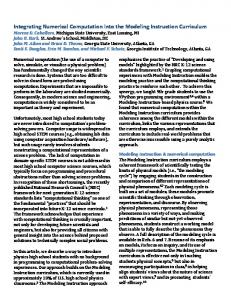
Chapter 1. Introduction 2005, Gupta et al., 2011], and a summary of the most relevant elements is presented below. • Al is one of the most common alloying elements. Addition of Al results in the enhancement of hardness and strength. It also improves castability. The alloys with more than 6 wt% of aluminum can be heat treated. • The addition of Mn enhances the saltwater corrosion resistance of Mg-Al and MgAl-Zn alloys. The low solubility of Mn in Mg limits the amount of Mn that can be added. Mn is usually incorporated with other alloying elements like aluminum. • Rare earths, as Nd, Ce, La, Yt, are added to increase the strength (specially at high temperature), creep and corrosion resistance. Furthermore, it has been observed [HerreraSolaz et al., 2014a] that the RE additions have an effect on the recrystallization process after forming, leading to more random textures. Their use is limited to high-added value applications, as rare earths are expensive. • Zn is usually used together with Al to increase the strength without reducing ductility. Moreover, the presence of Zn with Ni and Fe impurities can also assist to improve the corrosion resistance. • Zr acts as an excellent grain refiner when incorporated into alloys containing Zn, Th, rare earths, or a combination of these elements. However, it cannot be used with Al or Mn because of the formation of stable intermetallic compounds with these alloying elements. The mechanical properties of Mg alloys can be greatly improved by adding alloying elements by means of solid solution and precipitation hardening. As a result, Mg alloys are currently used in non-structural applications in different sectors including automotive, aerospace, health care, sports, electronics, etc. [Gupta et al., 2011]. Regarding automotive applications, Mg has been used in commercial vehicles since the 1930s in the Volkswagen Beetle, that already contained more than 20 kg of Mg alloys in the transmission housing and the crankcase. More recently, the environmental and legislative pressure on the automotive industry to produce lighter and more efficient vehicles have resulted in the surge of the use of light alloys. Widely used conventional steel parts are being replaced by new advanced materials such as Mg, Al, and metal-matrix composites. The most common applications of Mg alloys can be found in parts without structural responsibility like wheel assembly, gearbox housing and steering wheels (Fig. 1.1(a)), and they are starting to be used in interior parts such as the seat frame (Fig. 1.1(b)), steering column housing, driver’s airbag housing, and lock body [Kim and Han, 2008]. With respect to aerospace applications, weight reduction is one of the most critical 2

1.1 Importance of Mg alloys

(a)

(b)

(c)

(d)

(e) Figure 1.1: Steering wheel of the US Toyota Camry (a), Faurecia’s front seat frame platforms developed and produced for Nissan, General Motors and Volkswagen (b), Boeing 737 thrust reverser (c), Toshiba Portege Z830 − 104 with magnesium alloy chassis (d), Bike with a frameset and wheels that are injection metal molded in Mg (e)

objectives due to the increasing need for emission reduction and fuel efficiency. Over the years, Mg alloys have been used in both civil and military aircraft. Some applications 3

Chapter 1. Introduction include the thrust reversal (for several Boeing, Fig. 1.1(c)), gearbox (Rolls-Royce), and helicopter transmission casings. Mg alloys are becoming increasingly attractive for the aerospace industry after the recent release by the Federal American Aviation (FAA) of a report required to get Mg in the cabin of aircraft under special conditions approvals. However, its application in structural parts replacing Ti or Al alloys is still under investigation. Mg alloys have also been used in health care. They were introduced as orthopedic biomaterials in the first half of the last century [Earl D. Mcbride, 1938]. However, its use has been limited because of its low corrosion resistance. Despite this, Mg is very attractive for bone replacement in biomedical applications because its elastic modulus, compressive strength and density are closer to those of natural bone than any other metallic material [Staiger et al., 2006], while its fracture toughness is much higher than that of hydroxyapatite. In addition, Mg has good biocompatibility and it is biodegradable in human body fluid by corrosion, thus eliminating the need for another operation to remove the implant. All these features indicate that Mg are very promising materials for implants [Song et al., 2008, 2009]. The excellent ability of Mg alloys and Mg composites to be processed by die casting into intricate shapes resulted in many applications in sports equipment and electronics devices. They include the handles of archery bows, tennis rackets, golf clubs, bicycle frames (Fig. 1.1(e)), housings of cell phones and cameras, computers, laptops (Fig. 1.1(d)), and portable media players. Many more applications in structural components are envisaged for Mg in the future if the difficulties associated with corrosion resistance and limited mechanical properties are overcome. Although the mechanical properties of Mg alloys have been studied for many decades, the body of knowledge on this material is much more limited than that for steel or Al alloys. There is a lack of fundamental understanding of the key factors controlling the macroscopic mechanical behavior of Mg and its alloys and this information is critical to design novel alloys with improved microstructure. This situation is changing rapidly due to the development of novel experimental techniques to characterize the microstructure and the deformation mechanisms at the microscopic scale (electron backscatter diffraction, X-ray computed tomography, in situ mechanical tests, etc.) and of advanced numerical simulation tools (crystal plasticity, computational homogenization) that can provide a detailed picture of the dominant deformation and fracture mechanisms in Mg as a function of the loading conditions. 4

1.2 Deformation mechanisms of Mg alloys

1.2

Deformation mechanisms of Mg alloys

Mg single crystals present a hexagonal closed packed (HCP) lattice, similar to that of Be, Cd, Ti, Zn and Zr. The unit cell of the HCP lattice is a hexagonal prism which has two hexagonal bases with sides of length a and height equal to c. Each vertex and the center of these bases are occupied by one atom and a triangle of 3 atoms is also placed between these 2 planes, see Fig. 1.2. The c/a ratio of Mg single crystals is 1.624, very close to the theoretical value of 1.633 for contacting spheres. Crystallographic features of HCP crystals, such as vectors and atomic plane families, can be described using a four-value Miller index notation (hkil) in which the third index i denotes a convenient but degenerate component which is the negative of the sum of the first two (i = −h − k). The h, k and i index directions are separated by 120◦ and are parallel to the axes a1, a2 and a3 in the basal plane of the prism. The l component is perpendicular to the basal plane and parallel to the vertical axis c [Bravais, 1850] (Fig. 1.3 left side).

(a)

(b) Figure 1.2: HCP crystallographic structure

The elastic behavior of Mg single crystals presents transversely isotropic symmetry due to the HCP lattice. The stiffness tensor C that relates the stress tensor S with the elastic strain tensor Ee (S=CEe ) can be characterized by means of the 5 independent elastic constants C1111 , C1122 , C1133 , C3333 and C1212 , being direction 2 parallel to a2 and direction 3 to c. The corresponding values are shown in Table 1.1 [Slutsky and Garland, 1957]. 5

Chapter 1. Introduction C1111

C1122

C1133

C3333

C1212

59.4

25.6

21.4

61.6

16.4

Table 1.1: Elastic constants (in GPa) of Mg single crystal at 300K [Slutsky and Garland, 1957].

Plastic deformation, contrary to elastic deformation, is irreversible and two main plastic deformation mechanisms can be found in Mg, namely dislocation slip and twinning, Fig. 1.4(a). Plastic deformation by slip is due to the movement of dislocations in the atomic planes with the highest atomic density and along the closed-packed orientations. They correspond to the basal plane in Mg in three different orientations, namely h2¯1¯10i, h¯12¯10i and h¯1¯120i. However, five independent slip systems are necessary to accommodate general plastic deformation of the lattice [Taylor, 1938, Bishop and Hill, 1951] and basal slip can only provide two. Thus, plastic deformation in other crystallographic planes with lower atomic density is also necessary in HCP metals. In the case of Mg and Mg alloys, these systems are, prismatic slip ({10¯10}h¯12¯10i) and pyramidal hai ({10¯11}h¯12¯10i) or hc+ai ({10¯10}h¯12¯10i), that are also represented on Fig. 1.3.

Figure 1.3: Plastic deformation modes in Mg

In addition to dislocation slip, plastic deformation in Mg (and other low symmetry crystal structures) can occur by twinning, providing an additional mechanism to accommodate c-axis deformation. The availability of twinning deformation modes in HCP is intimately tied to the c/a ratio [Yoo, 1981]. A mechanical twin formally corresponds to a sheared volume for which the lattice orientation is transformed into its mirror image across a so-called twin or habitus plane (oblique dividing plane defined by the twinning 6

1.2 Deformation mechanisms of Mg alloys direction, see Fig. 1.4 right). The sheared region of the crystal undergoes an irreversible shear deformation of 0.129 [Zhang and Joshi, 2012]. Twins are easily observed by optical microscopy as thin lines within the grains which divide the twinned region from the rest of the crystal. The crystallographic orientation of the crystal within the twinned region is different from that of the parent grain and this is readily observed by means of electron backscatter diffraction (EBSD), as shown in Fig. 1.5. The development of twinning is a process that involves two steps. The first one is the propagation of a thin twin band across the grain, starting normally from the grain boundary. Afterwards, the twinned region propagates in the direction perpendicular to the twin plane and eventually the twinned region occupies most of the parent grain. Two different twining modes have been reported in Mg, namely extension or tensile twinning ({10¯12}h¯1011i) (the most commonly observed), that appears when the c axis ¯ ¯1¯1¯3i) (less comexperiences tension, and contraction or compressive twinning ({21¯12}h2 mon), that occurs under compression along the c axis [Reed-Hill and Robertson, 1957a,b, Yoshinaga et al., 1973]. Contrary to plastic slip that may occur in either direction of the slip vector, tension twinning only occurs in the direction that promotes the extension of the c axis, while compression twinning takes place in the direction that leads to compression of the c axis. Thus, twinning –as opposed to dislocation slip – is a polar deformation mechanism.

Figure 1.4: Permanent deformation after by slip and twinning.

7

Chapter 1. Introduction

Figure 1.5: EBSD image of Rh showing twins within the grains. [Kacher and Minor, 2014]

Plastic deformation in a given slip system is activated when the resolved shear stress, τ α reaches a critical value, the critical resolved shear stress (CRSS, τcα ), a material parameter which depends on the chemistry, microstructure and deformation stage of the crystal. The resolved shear stress on the system α (τ α ) is obtained by the projection of the stress tensor S on the corresponding slip plane defined by its plane normal n and slip direction s, according to τα = S : s ⊗ n

(1.1)

In the case of a uniaxial loading, the plane normal (n) and the slip direction (s) are given by the angles λ and ϕ (Fig. 1.6), and equation 1.1 is simplified to τ α = σ cos(λ) cos(ϕ)

(1.2)

where m∗ = cos(λ) cos(ϕ) is the so-called Schmid factor. Regarding twinning activation, the present trend follows the seminal developments by Kalidindi [1998], Salem et al. [2005] and Staroselsky and Anand [1998] who included twinning along with slip within the constitutive equation. This approach introduced twinninginduced plasticity through a phenomenological evolution law for the twin volume fraction. Twinning is modeled as a pseudo-slip mechanism and its activation is controlled by a CRSS 8

1.2 Deformation mechanisms of Mg alloys

Figure 1.6: Geometric configuration to determine the resolved shear stress τ α on the slip system characterized by the normal plane n and the slip direction s under uniaxial loading σapplied .

acting on the habitus twin plane and along the twinning direction and taking into account the polar nature of twinning. In Mg alloys, the CRSS of compression twinning is 15 times higher than that for tensile twining and, thus, very often only tensile twinning is activated during deformation of Mg and Mg alloys [Zhang and Joshi, 2012]. In cubic materials (either FCC or BCC), general plastic deformation can be accommodated by one single slip system. In the case of Mg, the critical resolved shear stress for the basal mode is much smaller than those of the other slip modes, but basal slip can only provide two independent slip systems and cannot accommodate general plastic deformation. This leads to the activation of twinning to accommodate the deformation perpendicular to the basal plane, being basal slip and tensile twinning the most active deformation modes in pure Mg and most Mg alloys because the CRSSs to active prismatic or pyramidal slip are much higher. This trend may be affected, however, by the alloying elements or temperature leading to changes in the most active modes. Rolled Mg and Mg sheets present a marked basal texture and the c axis of the Mg 9

Chapter 1. Introduction hexagonal crystals is aligned with the normal direction (ND) that is perpendicular to the rolling direction (RD), see Fig. 1.7. The pole figure characteristic of this texture is depicted in Fig. 1.7 left, where the accumulation of grains in ND shows the orientation of the c axis along this direction.

Figure 1.7: (Left) Typical pole figure of rolled Mg along ND direction. (Right) Section A-A corresponding with the plane defined by RD-ND axes. [Zhang and Joshi, 2012]

Under these conditions, the plastic deformation may be dramatically different depending on the loading direction, Fig. 1.8(a). This is depicted in Fig. 1.8(b), which shows the tensile stress-strain curves of rolled AZ31 Mg alloy along different orientations with respect to the normal direction, ND (from 0◦ to 90◦ ) [Liu et al., 2011]. Specimens tested along an angle between 0◦ to 30◦ with respect to ND showed relatively lower yield strength due to activation of extension twinning together with basal slip. In addition, the stress-strain curves when twinning is active, present a particular “concave up” shape. This is due to the progressive increases of twin volume fraction and to the final exhaustion when the most part of the material has been transformed. When angles are larger than 60◦ , basal slip and pyramidal slip are the dominant deformation modes. The reason of that was that rolling processes provokes that the vertical orientation of the crystals (parallel to c) is the ND, favoring therefore the twinning activation when the tensile tests are performed in ND and its inhibition when they are oriented with 90◦ to ND. [Jiang et al., 2008]. 10

1.3 Modeling of polycrystal behavior

(a)

(b)

Figure 1.8: (a) Orientation of the tensile axis with respect to the normal direction ND. (b) Representative stress-strain curves of specimens tested at different angles with respect to ND [Liu et al., 2011]

1.3

Modeling of polycrystal behavior

Structural components of metallic materials are made up of polycrystalline alloys. Polycrystal homogenization provides a bridge between micro and macroscale by means of integration of the microscopic strain and stress fields within the different grains to obtain the macroscopic stresses and strains in the polycrystal. This kind of approach is applicable to problems with a clear separation of scales, i.e. those in which the typical length-scale associated with the gradients of the mechanical fields at the macroscale is large compared with the typical length-scale of the polycrystalline microstructure (e.g. the grain or sub-grain size). Within this framework, the influence of the microscopic features of the polycrystal (grain size, shape and orientations as well as elastic constants and the CRSS of the different slip and twinning modes) on the macroscopic response can be taken into account. Polycrystal homogenization is a very complex, non-linear problem that has been solved with two different approximations, namely mean-field methods [Taylor, 1938, Sachs, 1928, Molinari et al., 1987, Lebensohn and Tomé, 1993] and computational homogenization [Miehe et al., 1999, 2002, Michel et al., 1999, Lebensohn et al., 2011, Segurado and Llorca, 2013]. Both of them rely on the definition of a Representative Volume Element (RVE) of the microstructure, a crucial element to bridge micro and macroscales. 11

Chapter 1. Introduction

1.3.1

Representative volume element

The RVE is a sample of a heterogeneous material that fulfills the following conditions:

• It is entirely representative of the microstructure on average, and • it is sufficiently large for the apparent properties to be independent of the surface values of traction and displacement, so long as these values are macroscopically uniform [Hill, 1963]. In essence, the first statement is about the material’s statistics (i.e. spatially homogeneous and ergodic), while the second one is a pronouncement on the independence of effective constitutive response with respect to the applied boundary conditions. In the case of polycrystals, the RVE is the smallest number of grains over which a measurement can be made that will yield a value representative of the whole polycrystal. A simple periodic unit cell is the RVE in the case of materials with periodic microstructure (Fig. 1.9(a)), but the situation becomes much more complicated in random media, and 2D or 3D complex cells which contain grains with different sizes, shapes and orientations are necessary (Fig. 1.9(b)). Very accurate data can be currently obtained of the grain size, shape and orientation in polycrystals owing to the development of advanced 3D microstructural characterization techniques (such as serial sectioning and X-ray microtomography together with electron back-scattered diffraction and X-ray diffraction) [Ludwig et al., 2009, Robertson et al., 2011, Fernández et al., 2013, Sket et al., 2014]. Grain size and shape statistical functions, together with the orientation distribution function (that characterizes the texture) can be used by means of Monte Carlo lotteries to build up RVEs of the polycrystal microstructure. The second key ingredient to simulate the polycrystal behavior is the complex behavior of the single crystals, which should include both plastic deformation by slip and twinning in the case of Mg. The framework for this task is the well established crystal plasticity theory [Kr¨ oner, 1961, Mandel, 1972, Asaro and Rice, 1977], to describe the homogeneous and heterogeneous deformation and hardening of single crystals under complex loading conditions. 12

1.3 Modeling of polycrystal behavior

(a)

(b) Figure 1.9: Periodic microstructure and the corresponding RVE (a). Random polycrystal microstructure and the corresponding RVE (taken from [Segurado and Llorca, 2013]).

1.3.2

Crystal plasticity model

Crystal plasticity estimates the plastic deformation that undergoes a single crystal under certain boundary conditions. Because plastic deformation, specially under forming process, can be substantially large, the kinematics of crystal deformation under finite strains should be established previously. A region in the three-dimensional space R3 is assigned to the material body B. The points within this region are called particles or material points. Different configurations or states of the body correspond to different regions in the 3D space. B0 and B are the undeformed and deformed configuration at times t0 and t, respectively (Fig. 1.10). The positions of the material points in the undeformed (or reference) configuration are given by vector x, whereas those in the deformed (or current) configuration are denoted by y. 13

Chapter 1. Introduction Thus, the displacement in the deformed configuration is given by u = y − x.

Figure 1.10: Reference or undeformed configuration (B0 ) and current or deformed configuration (B). Notation.

The deformation dy of a material line segment dx at x in the reference configuration is given by means of the deformation gradient tensor F as follows ∂y dx = Fdx ∂x The velocity of the material point x is given by dy =

(1.3)

d u = u˙ (1.4) dt and the velocity gradient L, which expressed the relative velocity between two positions in v=

the deformed configuration, can be expressed as function of deformation gradient F as, ∂v ˙ −1 = FF (1.5) ∂y The elasto-plastic deformation of the single crystal is accounted for by means of the L=

multiplicative decomposition [Kr¨ oner, 1961]. The single crystal deformation can be decomposed into two components Fe and Fp , see Fig. 2.1. The elastic deformation gradient, Fe , includes the recoverable distortion of the lattice as well as the rigid-body rotations while Fp accounts for the irreversible plastic deformation induced by plastic slip and twinning. In this sense, transformation of the reference state by Fp leads to an intermediate configuration, Bint , corresponding to a fictitious state of the body in which each material point 14

1.3 Modeling of polycrystal behavior is unloaded and with its particular lattice coordinate system coinciding with the system in which the constitutive equations are written.

Figure 1.11: Multiplicative decomposition of the total deformation gradient F into the elastic, Fe , and plastic, Fp , components.

The transformation from the reference configuration to this intermediate configuration hence needs to include the flow of material expressed in the constant lattice frame. The subsequent transformation from the intermediate to the current configuration, corresponding to elastic stretching of the lattice (plus rigid-body rotations), is characterized by the elastic deformation Fe . Therefore, the overall deformation gradient relating the reference to the current configuration follows from the sequence of both contributions as F = Fe Fp

(1.6)

The evolution of the plastic deformation gradient Fp can be expressed as function of velocity gradient Lp , following the definition 1.5 applied to Fp , leading to F˙p = Lp Fp

(1.7)

and it can be expressed as [Rice, 1971], Lp =

N X

γ˙ α sα ⊗ nα

α=1

15

(1.8)

Chapter 1. Introduction if plastic deformation takes place by dislocation slip. The vectors sα and nα stand, respectively, for unit vectors in the slip direction and the normal to the slip plane of the slip system α and N is the number of slip systems. The term γ˙ α is the shear rate for the system α which is a function of the resolved shear stress, τ α , and the critical resolved shear stress, τcα γ˙ α = f (τ α , τcα )

(1.9)

τ α = S : (sα ⊗ nα )

(1.10)

τcα = g(γ, γ) ˙

(1.11)

with

where S is the second Piola-Kirchhoff stress tensor and γ and γ˙ stand for the total shear strain on each system and the shear strain rate, respectively. Equations 1.8,1.9 and 1.11 will be reviewed in more detail in Chapter 3, where this model will be particularized for Mg alloys.

1.3.3

Mean-field approximations

Both mean-field approximations and computational homogenization are built upon the assumption of separation of scales illustrated in Fig. 1.12. The constitutive response of material in the macroscale is obtained by solving a boundary value problem in a representative volume element of this microstructure given by the subdomain β0 . The macroscopic (or effective) constitutive equation is given by the relation between S (the effective first Piola-Kirchhoff stress tensor) and F (the effective deformation gradient tensor). They can be expressed as 1 F= V0

Z

1 S= V0

Z

F(x)dV0

(1.12)

S(x)dV0

(1.13)

β0

β0

The mean-field approximation considers that the microfields in each grain can be represented by a single value, that is the volume-average of the corresponding microfield inside the crystal. Usually, the microstructure defined in the subdomain β0 is made then by a set of M inclusions βi inside a matrix, whose size, shape and orientation correspond to the 16

1.3 Modeling of polycrystal behavior Mean field subdomain 𝜷𝟎

𝑥

Polycrystalline microstructure at material point 𝒙

Macroscale Sample

Computational subdomain 𝜷𝟎

Figure 1.12: Separation of scales between microscale and macroscale.

single crystals in the polycrystal. The effective stress and strain deformation tensors can be expressed as M Z M 1 X 1 X F= FdVi = Vi hFi i V0 i βi V0 i

(1.14)

M Z M 1 X 1 X S= SdV0 = Vi hSi i V0 i βi V0 i

(1.15)

where hFi i and hSi i stand for the volume-averaged deformation gradient and stress tensor, respectively, in inclusion i and Vi for the volume of inclusion i in the subdomain. The different mean-field approximations adopt different hypothesis for the magnitude of hFi i or hSi i. The most simple ones are the isostrain (hFi i = F) or isostress approaches (hSi i = S). The first one assumes that all the inclusions undergo the same deformation while the second one proposes that the stress carried by all inclusions is equivalent. Both models were developed, respectively, by Taylor [1938] and Sachs [1928]. They are based on assumptions that disregard the shape and local neighborhood of the inclusions 17

Chapter 1. Introduction and generally violate equilibrium and compatibility conditions, respectively. These models may provide relatively accurate approximations of the polycrystal behavior if the single crystals are almost isotropic and posses a large number of slip systems to accommodate the deformation (FCC and BCC materials), but fail if there are large differences in the strains or stresses carried by individual grains, as it turns out to be the case in HCP crystals. Furthermore, although the isostrain approach fulfills the compatibility condition, leads to a very stiff response. More accurate models were developed in the context of Eshelby’s approach [Eshelby, 1957] and of particular linearization schemes to obtain the polycrystal behavior. Among them, the viscoplastic self-consistent scheme (VPSC) has become the standard tool to homogenize the plastic deformation of polycrystals. This formulation, based on a ad-hoc linearization of the non-linear single crystal constitutive behavior and on the use of the linear self-consistent approximation, was first proposed by Molinari et al. [Molinari et al., 1987] to predict the texture evolution of polycrystalline materials, and it was later extended and implemented numerically by Lebensohn and Tomé [Lebensohn and Tomé, 1993] in the so-called VPSC code. The main features of the VPSC strategy will be briefly reviewed below. The VPSC model assumes that the interaction of a grain with the surrounding matrix can be approximated by the interaction between the grain and a hypothetical homogeneous medium (HEM), which is characterized by an average constitutive behavior of the entire polycrystal aggregate. Each grain corresponds to a particular orientation of the ODF and its 2. volume fraction is taken as weightas of FE thatmaterial particular orientation Implementation oftheVPSC model in the ODF. The grains are represented as ellipsoidal inclusions, Fig. 1.13.

σ 'px

≈

+

grain

+…

σ 'px

HEM inclusion problem→ Eshelby

solution: linear ! Figure 1.13: VPSC assupmtion where the matrix-grain interaction is approximated by

Gran: a ellipsoidal grain (with its particular orientation) within a HEM linearization !

HEM: ε& VPSC p

=M

VPSC

:σ

app

Self-consistent equations: M

+ ε& op

VPSC

18

?? g

= M :B

g

=

∂ε& VPSC p ∂σ

localization tensors: f (Mg,MVPSC,Eshelby tensor)

1.3 Modeling of polycrystal behavior In contrast to Taylor or Sachs approaches, the relation between the crystal microfields ( 0c

σ and ˙ c ) and the average polycrystal macroscopic fields ( σ 0 px ˙px ) in VPSC, is different for each crystal and depends on the particular orientation of the crystal with respect to the HEM, Fig. 1.13. The standard version of VPSC is rigid-viscoplastic, an elastic stresses are neglected at both macroscopic polycrystalline and grain levels. Following this assumption, the macroscopic or polycrystalline deviatoric strain rate tensor ˙px is related to a macroscopic deviatoric stress tensor σ 0 px through a non-linear viscous relation. This non-linear relation is linearized at a given stress by ˙px = Mpx : σ 0

px

+ ˙px 0

(1.16)

where Mpx and ˙px 0 stand for the tangent viscoplastic compliance and the back-extrapolated strain rate, respectively. On the microscale, following the mean field assumptions, the behavior of each crystal (or orientation) c is solely represented by its average fields ˙ c and σ 0 c . The constitutive relation assumed for the whole grain is a power-law viscoplastic relation given by, n N 0c X σ : (sα(c) ⊗ nα(c) )Sym (sα(c) ⊗ nα(c) )Sym ˙ = γ˙0 α τ c α=1 c

(1.17)

where sα(c) and nα(c) are the tangent and normal vectors of the system α of grain c, (sα(c) ⊗ nα(c) )Sym is the symmetric Schmid tensor, τcα is the CRSS of system α in grain c and γ˙0 and n stand for the reference strain rate and rate sensitivity exponent, respectively. This viscous relation in eq 1.17 for each grain c is also linearized as, c

˙ c = Mc : σ 0 + ˙ c0

(1.18)

where Mc and ˙ c0 stand for the tangent viscoplastic compliance and back extrapolated strain rate of grain c. The localization equations in a mean-field model provide the relationship between microfields and macrofields. In the VPSC approach, the localization stress tensors Bc and bc can be written as c

σ 0 = Bc (Mc , Mpx , S)σ 0

px

+ bc (Mc , Mpx , S, ˙0 , ˙ c0 )

(1.19)

where S is the Eshelby’s tensor. The Eshelby tensor S stands for an anisotropic ellipsoidal inclusion embedded in an anisotropic media and, contrary to the isotropic case, analytical 19

Chapter 1. Introduction expressions are not available. Thus, it has to be computed numerically for each orientation using Green functions. The particular expressions for the localization tensors Bc and bc can be found in the literature [Segurado et al., 2012, Lebensohn and Tomé, 1993] and are not given here for brevity. Polycrystalline fields can be obtained as an average over the crystal fields. For instance, in the case of strain rates, ˙px =< ˙ c >

(1.20)

Finally, combining expression 1.16, 1.18, 1.19 and 1.20, the following self consistent equations are obtained Mpx =< Mc : Bc >

(1.21)

c c ˙ c0 > (1.22) ˙px 0 =< M : b +

This implicit set of equations can be solved iteratively to obtain Mpx and ˙px 0 . The VPSC model is used to simulate the polycrystalline response and microfield evolution under a given strain or stress history. This history is discretized in increments to obtain both the macroscopic polycrystalline behavior and the microscopic (grain) fields.

1.3.4

Computational homogenization

Mean-field models (and, particularly, the VPSC approximation) have demonstrated their ability to predict the average flow stress and the texture evolution in polycrystals and they have been recently used to provide constitutive equations for these materials within the context of multiscale simulations [Segurado et al., 2012]. However, these models cannot capture the local stress and strain fields accurately (they generally use only a mean value to represent the distribution of fields inside the grain) and this may lead to large differences at the local level for highly anisotropic crystals. In addition, the statistical treatment of the microstructure does not allow to analyze the influence of the actual grain shape and local details of the grain spatial distribution (i.e. clusters of second phases or grain orientations, etc). Under these circumstances, more sophisticated models based on computational homogenization have to be used to capture these local effects. Computational homogenization is based on the numerical simulation of the mechanical behavior of a representative volume element (RVE) of the material microstructure. The numerical solution of the boundary problem is carried out using different techniques, which 20

1.4 Mechanical behavior of single crystals include the Fast Fourier Transform method [Michel et al., 1999], recently extended to viscoplastic polycrystals [Lebensohn et al., 2011], and the finite element method [Miehe et al., 1999, 2002]). Three different types of discretization of the RVE can be carried out. The first one is a voxel-based model in which the RVE is made up by a regular mesh of N × N × N cubic elements, Fig. 1.14(a). Each cubic element stands for a single crystalline grain and thus the model can include a large number of grains. While this is important from the statistical viewpoint, this representation of the microstructure leads to a poor description of the grain shape and of the strain fields within the grains. Another possibility to represent the microstructure is depicted in Fig. 1.14(b). The discretization is also carried out with cubic elements but each crystal was represented with many elements and, thus, the model includes information about the distribution of grain sizes and shapes within the polycrystal. In addition, complex deformation fields can be accounted for within each grain. Nevertheless, the jagged shape of the grain boundaries is not realistic and this leads to a third type or representation (Fig. 1.14(c)), in which each grain is a polyhedron which is obtained by means of a Voronoi tessellation. Each polyhedron is discretized with a finite element mesh to capture the stress and strain gradients within the crystal. This third representation of the microstructure is obviously more realistic but the higher cost (from the viewpoint of the generation of the microstructure and of the computational resources) is not always associated with a dramatic improvement in the accuracy of the predictions and the RVE in Fig. 1.14(b) is often preferred. From the viewpoint of the boundary conditions, it is nowadays well established that the best results are obtained if periodic boundary conditions are applied to the RVE [Segurado and Llorca, 2002] because the effective behavior derived under these conditions is always closer to the exact solution (obtained for an RVE of infinite size) than those obtained under imposed displacements or forces (Huet [1990], Hazanov and Huet [1994]). Further details about the periodic boundary conditions are explained in section 2.3.

1.4

Mechanical behavior of single crystals

The physical deformation mechanisms in metallic single crystals have been studied in detail and they are well understood. The elastic behavior is determined by the crystal symmetry and the corresponding elastic constants, which are well known. Plastic deformation 21

Polycrystalline homogenization • Polycrystal behavior is obtained by FEM analysis of a RVE of the microstructure Chapter 1. Introduction • Three type of periodic RVEs are considered:

(a)

(b) (c) • The grain orientations are generated by MC to be statistically Figure 1.14: Discretization of RVE of polycrystals. (a) Model with 1000 cubic voxels, in representative of ODF which each microstructures one stands for a single Model containingobtained 100 crystals • The of (b)3crystal. and (c)(b)are synthetically to fitdiscretized with 64000 voxels. (c) Model in which each crystal is represented by a polyhedron statistics on grain sizes and shapes obtained by means of a Voronoi tessellation. • Periodic boundary conditions are used and load history is introduced by 9 independent terms of F(t) and Σ(t) 3 Dream3D

is controlled by dislocation slip and, in some cases, by twinning and it can be highly dependent on the crystal orientation, leading to a strong anisotropy in the plastic response. The single crystal behavior is modeled within the continuum viewpoint with crystal plasticity models [Hill, 1966, Rice, 1971, Hill and Rice, 1972], which take into account the geometry of slip and/or twinning for each material and lattice configuration, see section 1.3.2. The response of each slip/twinning system is governed by the critical resolved shear stresses (CRSS) and its evolution with deformation is introduced by means of either phenomenological [Asaro and Needleman, 1985, Bassani and Wu, 1991] or physically-based models [Arsenlis and Parks, 2002, Cheong and Busso, 2004, Ma et al., 2006]. Thus, although the theoretical framework to simulate the mechanical behavior of single crystals is available, quantitative values of the parameters in these models are difficult to obtain experimentally, limiting the predictive capabilities of the polycrystal homogenization. There are three different approaches available to obtain the quantitative values of the parameters which control the single crystal behavior. The first one is to carry out simple mechanical tests of microscopic single crystals built from the polycrystal (see Gianola and Eberl [2009] for a review) by means of focus ion beam milling. The microscopic single crystals have often a circular section with a diameter in the range 1 to 10 µm and can be tested in compression with a flat punch in a nanoindenter. By choosing the orientation of the parent grain, compression tests can be carried out in particular orientations to activate only one slip system and thus to obtain the CRSS as well as the strain hardening of each 22

1.4 Mechanical behavior of single crystals slip system. However, this is particularly difficult in single crystals which present a strong plastic anisotropy (e.g. Mg) because deformation tend to be dominated by softest slip modes regardless of the initial orientation of the crystal [Prasad et al., 2014, Ye et al., 2011, Kim, 2011] (Fig. 1.15). Moreover, the quantitative values of the CRSS and of the strain hardening for each slip system cannot be directly used in the simulation of polycrystals because of the presence of size effects.

Figure 1.15: Mg micropillar after compression in a direction at 45◦ from the basal plane normal, showing slip along the basal plane. Courtesy of Yuan-Wei Edward Chang

An alternative strategy, experimentally less challenging, is based on the use of instrumented nanoindentation of single crystals with different orientation within the polycrystal [Liu et al., 2005, Eidel, 2011, Sánchez-Mart´ın et al., 2014]. Testing is very straight forward in this case but the interpretation of the experimental data to obtain the parameters which control the behavior of each slip/twinning system is difficult due to the complex stress state below the indenter and. In addition, nanoindentation results are also size dependent. Another methodology to obtain the single crystal properties is based on a multsicale modeling approach. In this case, the effect of alloying elements, precipitates or defects and dislocation-dislocation interactions on the CRSS and the subsequent hardening are accounted for using density-functional theory, molecular dynamics or dislocation dynamics. Successful examples of this methodology have appeared recently [Leyson et al., 2010, Barton et al., 2013] but they are still limited in terms of the mechanisms that can be accounted for and of the uncertainties associated with the bridge of time and length scales 23

Chapter 1. Introduction between the different simulation approaches. Thus, taking into account the limitations of experiments and theory, the most widely used strategy to obtain the single crystal properties is based on the calibration of the parameters which control the single crystal properties by fitting experimental results of polycrystals loaded in different orientations by means of simulations based on mean-field methods or computational homogenization . The main problem with this strategy is that the number of parameters to be determined for each single crystal is very large and finding the optimum parameter set is neither easy nor a unique result is guaranteed. In fact, it is not unusual to find that different authors report different (or even contradictory) values for similar materials. HCP metals are the most typical example of these shortcomings because of the large plastic anisotropy and the coexistence of slip and twinning during plastic deformation. For instance, Table 1.2 shows the magnitude of the initial CRSS reported by different groups for the most important slip modes (basal, prismatic and pyramidalhc+ai) and extension twinning in AZ31 Mg alloy. The differences are non negligible from the quantitative viewpoint and, in addition, some authors [Agnew et al., 2001, Liu et al., 2011] considered that the initial CRSS for tensile twinning was below the one for basal slip whereas basal was the softest mode in other studies [Fernández et al., 2011, Knezevic et al., 2010, Wang et al., 2010], following the behavior of pure Mg. Obviously, these differences have very large implications in the dominant deformation mechanisms (and in the texture development) during deformation and their origin is not easy to assess. Although disparities in grain size or processing parameters could explain some of the differences in the initial CRSS reported on the different studies, the spread in the corresponding experimental results is much smaller than the differences among the CRSS values. This fact suggests that the disparities in the values proposed for the CRSS should also be closely related to the methodology used for the model calibration.

1.5

Objectives and structure of the thesis

Polycrystal homogenization is a powerful tool to obtain the mechanical properties of polycrystalline alloys that relies in three ingredients: an accurate representation of the microstructure (included in the RVE), a robust homogenization strategy (either based on mean-field or computational methods) and accurate information about the single crystal mechanical properties within the polycrystal. A huge progress has been achieved in the 24

1.5 Objectives and structure of the thesis Deformation mode

reference Fernández et al.

Liu et al.

Knezevic et al.

Wang et al.

Agnew et al.

Basal

α

α

α

α

α

Prismatic

9α

2α

5α

5α

—

Pyramidalhc+ai

13α

15α

6α

8α

3α

Twinning

2α

0.7α

2α

2α

0.5α

α (MPa)

9

—

—

15

30

grain size (µm)

13

42

8

—

25-100

Table 1.2: Values of the initial CRSS for different slips modes and tensile twinning in AZ31 Mg alloy predicted by fitting experimental results on polycrystals with simulations based on mean-field methods or computational homogenization.

first two areas in the last decades and the Achilles’ heel of polycrystal homogenization is the lack of a robust methodology (either experimental, theoretical or mixed) to obtain accurate, quantitative values for the mechanical properties of the single crystal, including the CRSS of the different slip/twinning modes and the corresponding strain hardening rates. The standard approach to obtain this information is based in inverse analysis in which the single crystal properties are obtained by fitting the predictions the polycrystal homogenization model for different loading conditions to experimental results. This is normally carried out by a trial and error approach and the accuracy of the resulting parameters is often uncertain because the problem is highly nonlinear, the number of parameters to be determined for each single crystal is very large and a unique result is not always guaranteed. The main objective of this thesis is to develop a robust and reliable inverse optimization methodology to obtain the single crystal properties from the mechanical behavior of polycrystals, which can be applied to strongly anisotropic HCP metals deforming by slip and twinning. The polycrystal behavior will be obtained by means of the finite element simulation of an RVE of the microstructure and the inverse problem will be solved by means of the Levenberg-Marquardt method [Levenberg, 1944, Marquardt, 1963], which is recommended for general non-linear least squares problems in optimization literature [Dennis and Schnabel, 1996]. The robustness and accuracy of the methodology will be assessed by comparing the predictions provided by computational homogenization with independent experimental results. In addition, the influence of the input information on 25

Chapter 1. Introduction the accuracy of the results will be studied. This methodology will be applied to two Mg alloys of large technological interest. Firstly, heavily textured rolled AZ31 Mg sheets, whose mechanical behavior is strongly dependent on the orientation with respect to the rolling direction, will be analyzed. Secondly, MN10 and MN11 Mg alloys will be studied. These are rare earth-containing alloys which present a weaker texture and more limited differences among the CRSS of the different slip modes. To fulfill these objectives, the thesis is structured as follows. After the introduction, the second chapter presents the models and algorithms developed to perform the numerical simulation of Mg and its alloys. This chapter is structured in three sections. The first one is devoted to the crystal plasticity model adapted for Mg alloys. The second section presents the computational homogenization strategy for polycrystalline Mg alloys and the inverse optimization methodology is detailed in section 3. The next chapter presents the application of this methodology to Mg alloys and also includes the analysis of the robustness of the approach. Finally, the conclusions and the future work are summarized in chapter 4.

26

Chapter

2

Models and algorithms

2.1

Finite element crystal plasticity model

The mechanical behavior of polycrystalline Magnesium alloys can be predicted using homogenization models that provide the macroscopic response as function of the crystal behavior and the polycrystalline microstructure (grain size, shape and orientation distributions). In addition to the use of an appropriate homogenization technique (either mean-field models or computational homogenization), three elements are fundamental for an accurate prediction of the behavior of the polycrystal: (1) A constitutive model for the behavior of the grains that reproduces the actual deformation mechanisms of the crystal, (2) a realistic and representative description of the microstructure and (3), a set of parameters that accurately describe the deformation of grains using previous model. In this chapter, the models and algorithms developed to create a computational homogenization framework for predicting the behavior of Magnesium alloys will be described. With respect to the crystal behavior (1), the general crystal plasticity (CP) framework will be presented together with the description of the particular CP model developed for Mg and its numerical implementation in the finite element context. Next, the microstructure representation (2) and the computational homogenization technique will be presented. Finally, the development of an inverse optimization technique to obtain the crystal parameters of a Mg alloy (3) from actual microstructure and macroscopic tests will be described. 27

Chapter 2. Models and algorithms

2.2

Crystal plasticity model for Mg alloys

A crystal plasticity model has been developed and implemented as a user material subroutine (UMAT) in the finite element code ABAQUS [Abaqus, 2013]. The UMAT developed here for Mg alloys is based on the subroutine developed and implemented previously for Titanium [Segurado and Llorca, 2013]. The original model was able to account for crystals with different lattices (FCC, HCP, BCC) and several types of hardening laws but the only plastic deformation mechanism accounted for was dislocation slip. However, an accurate description of the crystalline deformation in Mg alloys should undoubtedly include twinning deformation. For this reason, the original model [Segurado and Llorca, 2013] has been enhanced to simulate the behavior of Mg alloys by including a model for twinning deformation and other particular issues as non-Schmid effects on CRSS. The crystal plasticity formulation proposed here is based on the multiplicative decomposition of the deformation gradient in its elastic and plastic parts, according to F = Fe Fp

(2.1)

The total velocity gradient L (eq. 1.5 in section 1.3.2) can then be expressed as ˙ −1 = F˙ e Fe−1 + Fe F˙ p Fp−1 Fe−1 L = FF

(2.2)

−1 where Lp = F˙ p Fp stands for the plastic velocity gradient in the intermediate or relaxed

configuration. The plastic deformation is accommodated by two deformation mechanisms, slip and twin, being Nsl and Ntw the total number of slip and twinning systems available, respectively. Twinning is included in the crystal plasticity framework using the model developed by Kalidindi [Kalidindi, 1998]. A material point is divided into two phases, a parent region and a twinned region (Fig. 2.1), which is formed by a maximum of Ntw subregions. Each subregion belongs to a given twinning system α and its volume fraction is f α . Thus, the P tw α parent region volume fraction is given by 1 − N α=1 f . Under this approach the material point can be considered as a composite material in which the iso-strain hypothesis holds (F and Fe are the same in all phases). The plastic deformation is the result of three mechanisms and the plastic velocity gradient in the intermediate configuration contains three terms, related with the slip, twinning and re-slip mechanisms, Lpsl , Lptw , and Lpre−sl respectively. 28

2.2 Crystal plasticity model for Mg alloys

Figure 2.1: Multiplicative decomposition indicating material point subdivision in parent and twin phases

Lp = Lpsl + Lptw + Lpre−sl

(2.3)

The slip in the parent phase, Lpsl , is given by Lpsl

X Nsl Ntw X α f γ˙ i sisl ⊗ nisl = 1− α=1

(2.4)

i=1

where sisl and nisl stand, respectively, for the unit vectors in the slip and normal direction to the slip plane considered in the intermediate configuration. The second contribution, Lptw , is the rate of deformation due to the twin transformation of a differential volume fraction of parent phase df α

Lptw =

Ntw X

f˙α γtw sαtw ⊗ nαtw

(2.5)

α=1

where f˙α = df α /dt is the rate of the volume fraction transformation in the twin system α, sαtw and nαtw are the unit vectors defining the twinning system and γtw is the characteristic shear of the twinning mode (in the case of tension twinning of Mg alloys, γtw =0.129, [Zhang and Joshi, 2012]). It is recalled that extension twinning is a polar mechanism and it will only take place when the applied deformation leads to extension of the c axis of the HCP lattice. Finally, the third contribution corresponds to the slip of the transformed regions (here denominated as re-slip), Lpre−sl , which can be expressed as, 29


Lpre−sl =

Ntw X

Nsl−tw

X

fα

! i∗

i∗

i∗

γ˙ ssl ⊗ nsl

(2.6)

i∗ =1

α=1 i∗

where si∗ sl and nsl stand for the unit vectors in the slip and normal directions to the slip system i considered and re-oriented due to the twinning transformation of that region. The reorientation is defined by a rotation tensor Qα Qα = 2nαtw ⊗ nαtw − I

(2.7)

where I is the second order identity tensor. It has been experimentally observed that the volume fraction of twinned regions in many Mg alloy [Fernández et al., 2013, Kalidindi, 1998, Rémy, 1981] reaches a maximum P around f α ≈ 0.80. Thus, the re-slip term is activated at a given material point when the volume fraction of the twinned material at this point reaches 0.80. The number of systems considered for re-slip, Nsl−tw , might be smaller than the number of original slip systems Nsl for computational efficiency. Then, the total number of re-slip systems (Nre−slip ) will be obtained by the product of the number of slip systems that can undergo re-slip (Nsl−tw ), and the number of twinning systems (Ntw ), that is: Nre−slip = Ntw Nsl−tw

(2.8)

The crystal was assumed to behave as an elasto-viscoplastic solid in which the plastic slip rate for a given slip system follows a power-law, according to [Hutchinson, 1976],

i

γ˙ = γ˙ 0

|τ i | τci

m1

sign(τ i )

(2.9)

where γ˙ 0 is a reference shear strain rate, τci the CRSS of the slip system i, m the ratesensitivity exponent and τ i the resolved shear stress on the slip system i. Similarly, the twinning rate on the twinning system α, f˙α , also follows a viscous law ˙α

f = f˙0

hτ α i τcα

m1

( with

hτ i =

τ if τ ≥ 0 0 if τ < 0

(2.10)

and the transformation rate is set equal to zero if the volume fraction of twinned material exceeds a saturation value of 0.80 [Kalidindi, 1998]. Mathematically, 30


f˙α = 0 if

Ntw X

f α ≥ 0.80

(2.11)

α=1

Because of the iso-strain approach, the parent and twinned phases at a given material point are deformed under the same F and Fe and they share the same elastic strain in the intermediate configuration, given here by the Green-Lagrange strain tensor, Ee , Ee =

1 eT e F F −I . 2

(2.12)

The symmetric second Piola-Kirchhoff stress tensor in the intermediate configuration, S, is obtained in this case from the volume-averaged stress tensors in the different phases Ntw Ntw X X α parent S= 1− f S + f α Sα α=1

(2.13)

α=1

and the stresses on the parent (Sparent ) and twinned (Sα ) phases are given by

Sparent = CEe Sα = Cα Ee

(2.14)

where C stands for the fourth order elastic stiffness tensor of the crystal in its original orientation and Cα are the corresponding stiffness tensors reoriented after twinning. They are given by, Cαijkl = Cαpqrs Qαip Qαjq Qαkr Qαls

(2.15)

The resolved shear stress on a slip (τ i ) or twinning (τ α ) system in the parent (i) region is obtained as, τ i = Sparent : sisl ⊗ nisl

with τ α = Sparent : sαtw ⊗ nαtw

(2.16) ∗

while the resolved shear stress on a slip system in the twinned region (τ i ) is given by, ∗

∗

∗

τ i = Sα : sisl ⊗ nisl Finally, the Cauchy stress can be approximated as 31

(2.17)


T

T

σ = J −1 Fe SFe ≈ Re SRe

(2.18)

under the assumption of small elastic deformations, where J = det(F) and Re stands for the orthogonal rotation tensor obtained by the polar decomposition of Fe . The last ingredient of the model consists on the evolution equations of the CRSSs of each system (terms τc in equations 2.9 and 2.10). The initial values (in absence of α i for a slip system i and or τ0,c previous plastic deformation) of the CRSSs are given by τ0,c

a twin system α, respectively. A phenomenological hardening model is considered for the evolution of the CRSSs, which is able to reproduce the different stages of single crystal deformation [Kothari and Anand, 1998]. The evolution of the CRSS τci , τcα , τci∗ for slip, twin and re-slip systems are then given by equations 2.19, 2.20 and 2.21, respectively,

τ˙ci

= qsl−sl

Nsl X

asl a Ntw X τj τ β tw β j h0j 1 − j h0tw 1 − tw |γ˙ | + qtw−sl |γ˙ | τsat τsat j=1 β=1 τ˙cα

Ntw X

a τ β tw ˙α h0tw 1 − tw f γtw = qtw−tw τ sat β=1 Nre−sl

∗ τ˙ci

= qsl−sl

X j=1

asl τj h0j 1 − j |γ˙ j | τsat

(2.19)

(2.20)

(2.21)

where the different parameters in these equations define the contributions arising from self hardening and latent hardening. The self hardening of a given slip (i) or twinning (α) system correspond to the evolution of the CRSS only due to plastic deformation on that particular system. This evolution is defined by three terms: the saturation stress, τsat , the initial hardening rate h0 and the hardening exponent a. The evolution of the CRSS (τc ) in a given system isolated is depicted in Fig. 2.2. This figure shows how the initial value of CRSS (τo,c ) evolves, with a initial tangent modulus of h0 , until it reaches the value of τsat . The latent-hardening contribution to slip due to slip in other systems is introduced with the coefficient qsl−sl whereas the contribution induced by twinning is given by qtw−sl . The model only takes into account the effect of twinning on slip and it is assumed that slip does not influence twinning (qsl−tw = 0) [Capolungo et al., 2009, Zhang and Joshi, 2012]. Three slip modes (basal, prismatic and first pyramidal hc+ai) and tensile twinning have been included in the model to simulate the deformation of AZ31, MN10 and MN11 Mg 32


Figure 2.2: CRSS evolution by hardening

alloys. These deformation modes are depicted in Fig. 1.3 on page 6, and defined according to its normal plane n (red line) and slip direction s (blue line). Each deformation mode comprises several slip/twin systems considering the lattice symmetry of an hexagonal cell and the resulting set of 24 systems are shown in Table 2.1, both expressed in Bravais notation (a1 ,a2 ,a3 ,c) and in an orthogonal reference system, more useful for the numerical implementation. The orthogonal system is defined by three vectors e1 , e2 , e3 , fixed to the hexagonal cell and defined as e1 =a2 ×c, e2 =a2 and e3 =c, Fig. 2.3.

Figure 2.3: Different reference systems used to characterize the planes in the hexagonal lattice. Bravais (left) and orthogonal reference system (right)

2.2.1

Time discretization

The non-linear global FE problem is solved by applying the boundary conditions (loads or displacements) as a function of a time. The solution is obtained by imposing global 33

Chapter 2. Models and algorithms Slip mode

Slip syst

Basal

1

0

0

nbrav 0

1

2

sbrav

Basal

2

0

0

0

1

Basal

3

0

0

0

1

Prismatic

1

1

0

-1

0

Prismatic

2

0

-1

1

0

nort

sort

-1

-1

0

0

0

1

-0.8661

0.5

0

-1

2

-1

0

0

0

1

-0.8661

-0.5

0

-1

-1

2

0

0

0

1

0

1

0

-1

2

-1

0

1

0

0

0

1

0

2

-1

-1

0

0.5

0.8661

0

-0.8661

0.5

0

Prismatic

3

-1

1

0

0

-1

-1

2

0

0.5

-0.8661

0

-0.8661

-0.5

0

Pyrhc + ai

1

1

0

-1

1

-1

-1

2

3

0.8823

0

0.4708

-0.4543

0.2623

0.8514

Pyrhc + ai

2

1

0

-1

1

-2

1

1

3

0.8823

0

0.4708

-0.4543

-0.2623

0.8514

Pyrhc + ai

3

0

-1

1

1

1

1

-2

3

0.4411

0.7641

0.4708

-0.4543

-0.2623

0.8514

Pyrhc + ai

4

0

-1

1

1

-1

2

-1

3

0.4411

0.7641

0.4708

0

-0.5246

0.8514

Pyrhc + ai

5

-1

1

0

1

2

-1

-1

3

-0.4411

0.7641

0.4708

0

0.5246

-0.8514

Pyrhc + ai

6

-1

1

0

1

1

-2

1

3

-0.4411

0.7641

0.4708

0.4543

-0.2623

0.8514

Pyrhc + ai

7

-1

0

1

1

2

-1

-1

3

0.8823

0

-0.4708

0.4543

0.2623

0.8514

Pyrhc + ai

8

-1

0

1

1

1

1

-2

3

0.8823

0

-0.4708

0.4543

-0.2623

0.8514

Pyrhc + ai

9

0

1

-1

1

-1

-1

2

3

0.4411

0.7641

-0.4708

0

0.5246

0.8514

Pyrhc + ai

10

0

1

-1

1

1

-2

1

3

0.4411

0.7641

-0.4708

0.4543

0.2623

0.8514

Pyrhc + ai

11

1

-1

0

1

-2

1

1

3

-0.4411

0.7641

-0.4708

0

0.5246

0.8514

Pyrhc + ai

12

1

-1

0

1

-1

2

-1

3

-0.4411

0.7641

-0.4708

-0.4543

0.2623

0.8514

Tensile Twin

1

1

0

-1

2

-1

0

1

1

0.6838

0

0.7298

-0.7298

0

0.6838

Tensile Twin

2

0

1

-1

2

0

-1

1

1

0.3419

0.5922

0.7298

-0.3649

-0.632

0.6838

Tensile Twin

3

-1

1

0

2

1

-1

0

1

-0.3419

0.5922

0.7298

0.3649

-0.632

0.6838

Tensile Twin

4

-1

0

1

2

1

0

-1

1

-0.6838

0

0.7298

0.7298

0

0.6838

Tensile Twin

5

0

-1

1

2

0

1

-1

1

-0.3419

-0.5922

0.7298

0.3649

0.632

0.6838

Tensile Twin

6

1

-1

0

2

-1

1

0

1

0.3419

-0.5922

0.7298

-0.3649

0.632

0.6838

Table 2.1: Deformation systems considered. Plane normals n and slip directions s are expressed both in the Bravais coordinated system (a1 , a2 , a3 , c) (sub-index the orthogonal system (e1 , e2 and e3 ) (sub-index

brav )

and in

ort )

equilibrium at the end of each increment. The global solution for each time increment is obtained iteratively using a Newton-Raphson approach. A schematic flow chart of the calculations is depicted in Fig. 2.4 in order to clarify the different loops described below. Each global iteration of the displacement vector corresponds, at the integration point level, to a given deformation gradient tensor, F. Let t be the time corresponding to the last converged increment, then, the variables Ft , Fet , Fpt and σ t (corresponding to total, elastic and plastic deformation gradients and Cauchy stress, respectively) are known at each integration point. In addition, the set of internal variables αt defining the CP hardening evolution are known at time t. At time t + ∆t, iterative predictions of the global displacement vector are obtained in 34

2.2 Crystal plasticity model for Mg alloys the context of the global Newton-Raphson scheme. A given global displacement prediction also corresponds to a prediction of the deformation gradient at each integration point Ft+∆t . The constitutive equation at that integration point determines the Cauchy stress, the updated internal variables and the material tangent stiffness matrix (σ t+∆t , αt+∆t and ∂∆σ , ∂∆

respectively) as function of the actual predictor Ft+∆t and the converged values of Fet

and αt . The crystal plasticity routine solves, using an implicit scheme, an algebraical non-linear set of equations resulting of the integration of eqs. 2.1, 2.2, 2.3, 2.9, 2.17, 2.19, 2.20 and 2.21, between t and t + ∆t. The inputs and outputs are: α } INPUTS: Ft , Fet , Ft+∆t , αt = {γti ,ftα , τc,t

OUTPUTS: Fet+∆t , σ t+∆t ,

∂∆σ , ∂∆

α αt+∆t = {γt+∆t , ...}

The starting point is the integration of the plastic velocity gradient (expression 2.3) between t and t + ∆t to obtain the plastic deformation gradient Z

t+∆t p

Z

L dt = t

t+∆t

F˙ p Fp−1 → Fp t+∆t = exp(∆tLp t+∆t )Fp t

(2.22)

t

where the tensorial function exp() corresponds to the exponential map operator, [Souza et al., 2008]. Combining equation 2.22 with the multiplicative decomposition, the elastic deformation gradient at t + ∆t can be written as Fe t+∆t = Fe0 exp(−∆tLp t+∆t )

(2.23)

e Fe0 = (Ft+∆t F−1 t )Ft .

(2.24)

where Fe0 corresponds to If Fe t+∆t is renamed simply as Fe , a tensorial residual equation can be written from 2.23 as R(Fe ) = Fe − Fe0 exp(−∆tLp (Fe )) = 0.

(2.25)

and the solution of this equation provides the value of Fe . If step increments are sufficiently small ∆tLp → I, and the exponential function can be approached by exp(−∆tLp ) ≈ I − ∆tLp

(2.26)

to reduce the computational cost. In this case, the alternative residual equation is given by R(Fe ) = Fe − Fe0 (I − ∆tLp (Fe )) = 0 35

(2.27)


INPUT: , ,

,

PRED

UMAT

,

( ,

,

)

)

‐

OUTPUT: ,

, ,

=

, (

(

NEW

YES

)

,

,

)