15 NOVEMBER 2008
5887
FIELD ET AL.
Midlatitude Cyclone Compositing to Constrain Climate Model Behavior Using Satellite Observations P. R. FIELD, A. GETTELMAN,
AND
R. B. NEALE
NCAR,* Boulder, Colorado
R. WOOD University of Washington, Seattle, Washington
P. J. RASCH
AND
H. MORRISON
NCAR,* Boulder, Colorado (Manuscript received 12 September 2007, in final form 21 February 2008) ABSTRACT Identical composite analysis of midlatitude cyclones over oceanic regions has been carried out on both output from the NCAR Community Atmosphere Model, version 3 (CAM3) and multisensor satellite data. By focusing on mean fields associated with a single phenomenon, the ability of the CAM3 to reproduce realistic midlatitude cyclones is critically appraised. A number of perturbations to the control model were tested against observations, including a candidate new microphysics package for the CAM. The new microphysics removes the temperature-dependent phase determination of the old scheme and introduces representations of microphysical processes to convert from one phase to another and from cloud to precipitation species. By subsampling composite cyclones based on systemwide mean strength (mean wind speed) and systemwide mean moisture the authors believe they are able to make meaningful like-with-like comparisons between observations and model output. All variations of the CAM tested overestimate the optical thickness of high-topped clouds in regions of precipitation. Over a system as a whole, the model can both over- and underestimate total high-topped cloud amounts. However, systemwide mean rainfall rates and composite structure appear to be in broad agreement with satellite estimates. When cyclone strength is taken into account, changes in moisture and rainfall rates from both satellite-derived observations and model output as a function of changes in sea surface temperature are in accordance with the Clausius– Clapeyron equation. The authors find that the proposed new microphysics package shows improvement to composite liquid water path fields and cloud amounts.
1. Introduction Climate prediction science depends upon the accuracy of numerical models representing a variety of physical processes operating on diverse spatial and temporal scales. Methods for testing climate models typically consist of comparisons of global maps of annual or seasonal means or zonal means (e.g., Weare 1993).
* The National Center for Atmospheric Research is sponsored by the National Science Foundation.
Corresponding author address: P. R. Field, NCAR, 3450 Mitchell Lane, Boulder, CO 80301. E-mail:
[email protected] DOI: 10.1175/2008JCLI2235.1 © 2008 American Meteorological Society
While zonal and global mean comparisons are valuable tools for assessing global models, it is not easy to determine whether any discrepancies are due to the model general circulation being in error or misrepresentation of smaller-scale phenomena. More recently, compositing as a function of 500-mb pressure tendency has become more popular (e.g., Norris and Weaver 2001; Bony et al. 2004). Such compositing methods are powerful both as diagnostics and in simplifying the complex behavior of global models. One way to focus model–observation comparisons is to use the technique of compositing applied to individual phenomena. Klein and Jakob (1999) carried out the first comparison between composite satellite and composite model output of midlatitude cyclones using the European Centre for
5888
JOURNAL OF CLIMATE
Medium-Range Weather Forecasts model. In this study we use a cyclone-relative compositing approach to assess the ability of the Community Atmosphere Model, version 3 (CAM3) to accurately represent the spatial structure of midlatitude cyclones and their dependence upon their thermodynamic and dynamic environment. Previous comparisons of satellite data and global model output have generally revealed bias in cloud representations. Norris and Weaver (2001) compared International Satellite Cloud Climatology Project (ISCCP) data with the National Center for Atmospheric Research (NCAR) Community Climate Model version 3 (CCM3). They showed that for Pacific summertime midlatitude regions the CCM3 overpredicts cloud top height and cloud optical thickness in regions of large-scale ascent, while they find the opposite for regions of subsidence. They attribute the overproduction of cloud in the regions of ascent to the lack of subgrid variability in vertical velocity and hence humidity. Similarly, Webb et al. (2001) and Lin and Zhang (2004) both compared ISCCP climatologies with various climate models and found at midlatitudes that the cloud optical thickness was overestimated for hightopped clouds. Klein and Jakob (1999) found that, while the model generally reproduced the various cloud types and their cyclone-relative positioning, the model exhibited differences to the observations when the optical thickness characteristics were assessed. The CAM3 hydrological behavior was recently reviewed by Hack et al. (2006). They note that CAM3 overpredicts cloud liquid water path (LWP) in the midlatitudes when compared to satellite-derived products—consistent with an overprediction of optical thickness of clouds in GCMs. In contrast, the zonally averaged precipitation rates from CAM3 are more similar to the Climate Prediction Center Merged Analysis of Precipitation (CMAP) product (Xie and Arkin 1997) at midlatitudes, although the maxima are more poleward in CAM3, suggestive of a poleward bias of the storm tracks. Similarly, the column-integrated water vapor from CAM3 in midlatitudes agrees to within 10% of the National Aeronautics and Space Administration Water Vapor Project (NVAP) product (Randel et al. 1996). The study of composite cyclones by Field and Wood (2007a, hereafter FW07) used satellite-derived observations to partition the cyclones. It was asserted that (i) on average a cyclone will exhibit similar precipitation and cloud structure to another cyclone if the thermodynamic and mesoscale dynamical environments are comparable; (ii) the thermodynamic and mesoscale dynamical environment for each cyclone can be categorized by two metrics that represent the mean atmospheric mois-
VOLUME 21
ture and the mean cyclone strength. They found that a simple warm conveyor belt model adequately described the change in cyclonewide mean rainfall rate as a function of cyclone moisture and strength. However, hightopped cloud was more complicated and was better correlated with cyclone strength than with moisture. In this study we have focused on comparing satellite observations and CAM3 representations of composited midlatitude cyclones. By compositing cyclones based on their strength and moisture we believe we are able to compare like with like. In this way we hope to be able to avoid any differences in climatologies (e.g., different storm tracks) between the model and the satellite observations. Section 2 briefly describes the CAM3 model and modifications that we have used. Section 3 outlines the compositing methodology. The satellite data used for comparison will be summarized in section 4, and the comparison with the model data will follow in section 5. The discussion and summary forms sections 6.
2. Model description a. CAM3 Control Collins et al. (2006) describes the current NCAR CAM3, but for the purposes of this paper we will outline some aspects of the microphysics implementation and treatment of cloud fraction that will be relevant to the discussion. The microphysical representation in CAM3 is described in detail by Rasch and Kristjansson (1998) and introduced a prognostic condensed water variable with diagnostic phase separation based on temperature such that the condensed water liquid fraction varies from 1.0 at ⫺10°C to 0.0 at ⫺40°C (⫺30°C in the original implementation). Each phase consists of a “cloud” species that has negligible fall speed and a “precipitation” species that has a fall speed appropriate for the phase. The cloud fraction approach used in the model is described by Zhang et al. (2003) and is a diagnostic scheme based on the Slingo (1980) quadratic cloud fraction relation with an associated critical gridbox-mean relative humidity for the existence of cloud. The model runs presented here have been made using the CAM3 finite volume dynamical core at a grid spacing of 0.9° latitude, 1.25° longitude, 26 vertical levels (surface to 3 mb) and a time step of 30 min. One run carried out using 4° by 5° grid spacing to assess the effect of resolution on cyclone representation in the CAM was used. The radiation scheme is described by Collins et al. (2006) and the overlap scheme assumed for the subgrid deployment of the clouds is an important aspect. For the experiments described here, the maximum-random overlap assumption was used.
15 NOVEMBER 2008
FIELD ET AL.
b. CAM3 modifications We ran a number of different configurations of the CAM3 in an attempt to attribute physical or model parameterization differences to resulting differences in the model output. The configurations are 1) Ssat: this is a modification of the cloud fraction scheme that requires greater gridbox relative humidity to produce the same cloud fraction as in the standard CAM3. This modification was used in Gettelman and Kinnison (2007) and is a variation of the Slingo (1980) cloud fraction scheme. In the original scheme (as implemented in CAM) cloud begins to form at a gridbox-mean relative humidity with respect to ice of 90% and covers 100% of the grid box when the relative humidity, with respect to ice (for T ⬍ ⫺30°C), reaches 100%. The modification has the effect, for temperatures colder than ⫺30°C, of increasing the critical relative humidity to form cloud when ice is present from 90% to 100% and complete cloud cover occurs when the relative humidity is 120% over ice. 2) 4 ⫻ 5: a low horizontal resolution run often used for paleoclimate investigations with a horizontal grid spacing of 4° in latitude and 5° in longitude. 3) Nodeep: the Zhang and McFarlane (1995) deep convection parameterization was turned off, with convection handled only by the “local” convective scheme (Hack 1994). 4) Noconv: both the deep and “local” subgrid convection schemes were disabled. 5) Micro: the microphysical scheme of Morrison and Gettelman (2008) was used. The new stratiform microphysics scheme in CAM predicts the number concentrations and mixing ratios of cloud droplets and cloud (small) ice. The prediction of both mixing ratio and number concentration allows the effective radius to evolve freely in the model, which is critical for cloud radiative forcing. The scheme also diagnoses both the mixing ratio and number concentration of rain and snow. This allows for the differentiation of precipitation regimes; namely, shallow clouds with drizzle versus deeper cloud systems with melted snow and large rain drops (Gettelman et al. 2008). The scheme includes a number of microphysical processes that transfer water between vapor, clouds, and precipitation (e.g., condensation, autoconversion, accretion). It also includes a physically based treatment of the partitioning between liquid and ice in subfreezing conditions based on the relevant process rates (freezing, riming, and the Bergeron process, that is, transfer of liquid to ice due to lower ice saturation vapor pressure).
5889
Other microphysics schemes in GCMs typically use simple temperature-based partitioning to separate liquid and ice (e.g., Del Genio et al. 1996; Rasch and Kristjansson 1998). When running the models with prescribed sea surface temperatures (SSTs), the global radiative balance of the model is not vital because the ocean acts as an infinite energy source/sink. However, the models need to be configured sufficiently well so that unrealistic global warming or cooling does not occur in fully coupled ocean–atmosphere runs. Therefore it is desirable that the atmospheric component of the model is in approximate global radiative balance at the top of the atmosphere. We note that model configurations Control, Ssat, 4 ⫻ 5, and Micro were run in approximate global radiative balance at the top of the atmosphere (⫾2 W m⫺2), while the Nodeep and Noconv configurations were not balanced radiatively (⫾10 W m⫺2). For the Control, Ssat, and 4 ⫻ 5 configurations the model was run for 10 years to establish a climatology. For the Nodeep, Noconv, and Micro configurations it was decided that 5 years would be sufficient owing to computational costs. For all configurations we analyzed the last three model years (36 ⫻ 30 days) of the data. All configurations were run as a stand-alone atmosphere with a predefined data ocean of observed SSTs. Because different years were used in the analysis of the model results and satellite data, we assessed any differences introduced by the variation in observed SSTs by comparing the Control run analysis for two different 3-yr periods. We found that using different years for the analysis did not introduce any biases that might arise from different SST climatologies. The results are discussed below in more detail.
3. Model output compositing From the final three years of the runs, daily instantaneous output was obtained at 0000 UTC for the following two-dimensional fields: mean sea level pressure, 10-m horizontal winds, integrated water vapor column, rainfall rate, liquid water path, sea surface temperature, integrated column relative humidity (FW07), cloud top temperature, and cloud types generated from the ISCCP simulator embedded in the CAM3 (Klein and Jakob 1999), which predicts what a satellite would see given subgrid assumptions such as cloud overlap geometries (assumed to be maximum random overlap in this case). We note that the ISCCP simulator only uses the parameters associated with nonprecipitable species to estimate the radiative effects of clouds. The satellite observations of clouds used for the comparison employ Moderate Resolution Imaging Spectroradiometer
5890
JOURNAL OF CLIMATE
(MODIS) data. MODIS can detect a minimum optical depth of 0.1–0.2 (Choi et al. 2005), so we have made use of all optical depth bins provided from the ISCCP simulator. For cloud types obtained with satellite data the pressure categories used were ptop ⬍ 440 hPa, 440 ⬍ ptop ⬍ 710 hPa, ptop ⬎ 710 hPa for high-, mid-, and low-top cloud respectively. Cloud optical depth thresholds used to classify clouds into optically thin, medium, and thick types are ⬍ 5, 5 ⬍ ⬍ 25, and ⬎ 25, respectively, for water clouds and ⬍ 3.75, 3.75 ⬍ ⬍ 25, and ⬎ 25 for ice clouds. These categories are slightly different to those used by ISCCP, but they are as close as is possible given the joint histogram bins used in the MODIS level 3 data (Oreopoulos 2005). For the CAM output we used the same pressure thresholds (emissivity-adjusted cloud top pressure) and the same optical thickness thresholds as used for the water clouds. The 10-m horizontal winds were computed using a two-stage iterative technique to compute correction factors for the lowest model layer winds to estimate the 10-m winds based on stability and the height of the lowest model layer (CCSM3.0, coupler v6.0 documentation, available online at http://www.ccsm.ucar.edu/ models/ccsm3.0/cpl6/). For compositing the model cyclones we followed the same method used for the satellite and reanalysis data (FW07). To locate the cyclones we used surface pressure and derived first- and second-order derivatives that were thresholded to obtain candidate grid points to represent the cyclone center (d 2p0⬘ /dxdy ⬍ 4 ⫻ 10⫺5 hPa2 km⫺2 and d 2p0⬘ /dx2 ⫹ d 2p⬘0 /dy2 ⬎ 9 ⫻ 10⫺5 hPa km⫺2). These candidates were then filtered to locate the maximum negative anomaly within a 1900-km radius with p0 ⬍ 1015 hPa (FW07 used 2000 km, but here we reduced it slightly to include slightly more cyclones per year). Therefore a single cyclone throughout its evolution could be identified as separate systems on consecutive days. From the global analysis of cyclone locations we focus the analysis in this paper upon four subregions: North Pacific (30°–55°N, 145°E–165°W); North Atlantic (30°–60°N, 10–50°W); South Pacific (30°–55°S, 120–180°W); South Atlantic (30°–55°S, 50°W–10°E). Cyclone centers must be located within these domains to be considered for analysis. For each cyclone the model output fields (initially all on a 0.9° ⫻ 1.25° grid, apart from the 4 ⫻ 5 runs) are translated and regridded using bilinear interpolation onto a 4000 km by 4000 km domain (x, y are the eastward and northward coordinates respectively) with 100km grid spacing and the cyclone located centrally (x ⫽ 0, y ⫽ 0). After regridding data onto the cyclone-centric do-
VOLUME 21
main, statistics are derived from the resulting ensemble of cyclones. We examine cyclone properties as a function of cyclone strength and atmospheric moisture metrics that are defined as follows: Cyclone strength, 具V 典, is determined as the mean 10-m wind speed, within a circle of radius 2000 km centered on the cyclone. Our atmospheric cyclone moisture metric is similarly defined as the mean water vapor path 具WVP典 within a circle of radius 2000 km centered on the cyclone. We choose a measure of the atmospheric moisture content as an additional metric because it determines the availability of moisture for the development of cloud and precipitation and it is strongly dependent on sea surface temperature (see FW07) and, so, will change with increasing global temperatures. Cyclones in the Southern Hemisphere are similar to their Northern Hemisphere counterparts for similar cyclone strength and atmospheric moisture (FW07). We therefore reflect the Southern Hemisphere cyclones about a zonal axis (x → x, y → ⫺y) and combine all of the cyclones in a Northern Hemisphere sense. Conditional sampling of the cyclones into three moisture categories (具WVP典: 10–18, 18–21, 21–33 kg m⫺2) and three strength categories (具V典: 4.9–6.95, 6.95–8.14, 8.14–12.3 m s⫺1) matching those used in FW07 produces nine composite categories. Further conditional sampling within an 具WVP典, 具V典 ellipse (see FW07) ensures that there is no monotonic variation in strength for a given strength category and different moisture categories or vice versa. The cyclone database is finally filtered to remove systems where the fraction of nonmissing SSTs colder than 278 K exceeds 0.3. This filtering is performed so that potential problems with the rain rate estimates related to near-surface freezing levels are avoided. Thus, the composite cyclones within each of the categories contain cyclones from all four oceanic regions at all times of year. Cyclone-wide composite means (within 2000 km radius of center) of a number of parameters have been generated. FW07 discussed systematic errors associated with the satellite measurements. Their conclusion was that, if there are no systematic biases in the observations, then given the number of observations combined at each point in the composites the random error is small (⬍1% for ⬃100 member composite). Therefore the error bars represent the standard error in the mean (in fact two times the standard error is plotted in the figures) due to variability from cyclone to cyclone. These errors are obtained by calculating the weighted mean of the standard error of the means at each point in the composite and then dividing by the square root of the degrees of freedom in the composite field (typically 5–20) that are determined using the spatial equivalent
15 NOVEMBER 2008
FIELD ET AL.
of the temporal autocorrelation method of Leith (1973).
4. Review of the satellite observations Here we briefly revisit the satellite data described in FW07 (and a correction that was issued: Field and Wood 2007b) that is used here for comparison. The main finding from the satellite observations is that the cyclonewide mean rainfall rates are consistent with a simple warm conveyor belt argument: Rwcb ⫽ c 具WVP典具V典,
共1兲
where c ⫽ wk/Ac is a constant (c ⫽ 0.023, Rwcb in mm day⫺1, 具WVP典 in kg m⫺2, and 具V 典 in m s⫺1) that is composed of the areal extent, Ac, of the cyclone (2000-km radius circle), the composite width, w, of the warm conveyor belt, and a constant, k. In FW07, c was found that provided the best correlation between the composite mean rain rate and the product of the composite mean moisture and strength. The observations showed that rain is generally located to the east of the cyclone center in a rough comma shape. The heaviest rain in the composite mean tends to occur just slightly northeast of the center and then arc around to the south, reminiscent of the warm conveyor structure suggested by Harrold (1973). In contrast to the behavior of the rainfall patterns with cyclone strength and moisture, the high-top cloud fraction was found to be positively correlated mainly with cyclone strength, exhibiting smaller variation with changes in moisture. This result was attributed to a possible decoupling between upper and lower tropospheric moisture.
5. Model–satellite comparisons Because we used two different groupings of years for the model analysis that are themselves different from the two years over which the satellite data were obtained, we would like to know if there is any effect introduced by the different SSTs that were present. As a test we carried out the same analysis of the Control run data for two different periods: 1979–81 and 1984– 86. We found that the distribution of cyclones within the nine strength and moisture categories was similar and that cyclone mean composite values for rainfall rate, high-topped cloud fraction, and RHcol (the ratio of the WVP to the saturated liquid water vapor path) are typically also very similar. In fact, t testing the cyclone mean composite values for rainfall rate and hightopped cloud fraction revealed that only 3 out of a total of 18 comparisons exhibited a difference significant
5891
at the 60% confidence level and none of means exhibited differences significant at the 70% confidence level. In some of the following figures we have plotted both Control run results to provide an estimate of variability introduced by using results from differing time periods. The formation of high clouds is a useful tuning process for climate models. By modifying the critical gridbox mean relative humidity (RHcrit) at which clouds begin to form, the amount of high cloud and, hence, the planetary albedo can be controlled. This effect can be used to fine-tune a climate model to balance the incoming and outgoing radiation. In the CAM the radiation only interacts with the nonprecipitating “cloud” ice and water. The condensed water in the precipitating species may have some impact on the optical thickness of clouds, but at present is not considered. Thus, there is a difference between what the CAM sees as radiatively important and what the actual cloudy atmosphere sees as radiatively important. The atmosphere sees a much wider range of hydrometeor sizes including precipitation particles. The model however, can have large cloud fractions generated by low water contents that may not be radiatively significant or seen by satellites. Figure 1 shows the composite-mean high cloud fractions for the greatest strength category and medium moisture category. The satellite data shows the “comma shaped” high cloud shield associated with the fronts out to the east of the cyclone center. All of the models capture this broad pattern, but the Control, Ssat, and especially the 4 ⫻ 5 runs produce too much high cloud. The result for Ssat is surprising given that greater relative humidity at temperatures colder than ⫺30°C is required to produce cloud. The Nodeep and Noconv runs are not radiatively balanced, but do produce less cloud. In these runs the removal of the model’s ability to respond to convective instability prevents transport of water vapor to the middle and upper troposphere. This results in less cloud and lower water vapor greenhouse effects, hence a large cooling to space and a radiative imbalance. The configuration is for illustrative purposes only and cannot represent a real moist atmosphere. The Micro run is radiatively balanced and produces less high-top cloud than the Control, but still more than the satellite observations suggest. We have examined these differences further by subdividing the high-topped cloud category into three optical thickness categories (Fig. 2, top left). We took all of the cyclones from the North Pacific region in the maximum strength minimum moisture category: the category that contained the highest proportion of model cyclones. The satellite observations show the largest contribution from the intermediate optical
5892
JOURNAL OF CLIMATE
VOLUME 21
FIG. 1. High-top (cloud top pressure ⬍440 mb) composite cloud fraction in each 100 km ⫻ 100 km grid cell for the satellite observations and different model configurations. The 4000 km ⫻ 4000 km domain composite is for the medium moisture, greatest strength category. The composite sea level pressure is overplotted (mb, solid lines).
thickness category. In contrast, all of the model results show that the contribution from the thickest cloud is most significant. For the Micro, 4 ⫻ 5, and Control there is also some contribution from the thinnest category. Similar figures have been generated for the midtop and low-top cloud categories, but interpreting the results for lower cloud tops is difficult because of the compounding masking effects of the higher clouds. Even though the ISCCP simulator does take account of cloud overlap, the cascade effect of the higher clouds can be difficult to unravel. Nevertheless, the models tend to produce less midtop cloud (Fig. 2, top right), while the satellite suggests 10%–20% cloud fractions of the intermediate optical thickness category to the west of the cyclone center. For the low-top cloud (Fig. 2, bottom) the models tend to overpredict the intermedi-
ate and greatest optical thickness cloud, while the satellite observations suggest modest amounts of optically thin low-top cloud. Returning to the total high-top cloud fraction we have plotted the composite mean values as a function of cyclone strength (Fig. 3) for the satellite and model results (the squares for the greatest strength category are obtained from the composite fields depicted in Fig. 2). Figure 3 shows that the 4 ⫻ 5 and Noconv runs are outliers that generate too much and too little high-top cloud amounts, respectively (see Table 1). For the other model configurations the agreement with the observations is better, but the Control appears slightly high. When viewing these cyclonewide composite means it is useful to consider the significance of any differences by referring to the t test. If we assume that the standard
15 NOVEMBER 2008
FIELD ET AL.
5893
FIG. 2. High-top (cloud top pressure ⬍440 mb) composite cloud fraction in each 100 km ⫻ 100 km grid cell for the satellite observations and different model configurations. The cloud fraction is broken down into three optical thickness categories: thin (cirrus ⬍ 5), intermediate (cirrostratus 5 ⬍ ⬍ 25), and thick (deep frontal ⬎ 25). Midtop (710 mb ⬎ cloud top pressure ⬎440 mb) composite cloud fraction in each 100 km ⫻ 100 km grid cell for the satellite observations and different model configurations. The cloud fraction is broken down into three optical thickness categories: thin (altocumulus), intermediate (altostratus), and thick (nimbostratus). Low-top (710 mb ⬍ cloud top pressure) composite cloud fraction in each 100 km ⫻ 100 km grid cell for the satellite observations and different model configurations. The cloud fraction is broken down into three optical thickness categories: thin (cumulus), intermediate (stratocumulus), and thick (stratus). The 4000 km ⫻ 4000 km domain composites are generated from all of the cyclones found in the North Pacific region.
error depicted in each plot (the plots show typical 2 times standard error estimates) is representative for all of the points, then the t statistic is simply the difference in the means divided by 公2 times the standard error.
The number of degrees of freedom for each point is greater than 100. Therefore, the t statistic for differences in the means of 1, 2, or 3 times the standard error is 0.7, 1.4, and 2.1, respectively. So, differences in means
5894
JOURNAL OF CLIMATE
VOLUME 21
FIG. 3. Mean composite high-top cloud fraction as a function of cyclone strength in the nine strength and moisture categories for the satellite observations and model configurations. The typical 2 times standard error in the mean is also indicated.
of 1, 2, or 3 times the standard error are different at the ⬃50%, ⬃85%, and ⬃95% confidence levels, respectively. Bearing in the mind the standard error in the mean, the results for Micro, Nodeep, and Ssat are in satisfactory agreement with the satellite observations (t statistics are given in Table 1). All model simulations correctly predict increasing high clouds with increasing cyclone strength, but the sensitivity in each case varies considerably. The difference between mean hightopped cloud fraction between the most moist and dry categories for a given strength category is about two standard errors, which means that their difference is only significant at the ⬃85% confidence level. However, this pattern is consistent for all three strength categories and from model to model, increasing the confidence level. Thus we can conclude that the model high-top cloud fractions vary more with moisture than the satellite observations. This point will be resumed in the discussion section. Rainfall rates derived from microwave measure-
ments are compared with the model results for the strongest strength category and the medium moisture category in Fig. 4. All show rain located in a commashaped region to the east and southeast of the cyclone center. The models show considerable skill in predicting the extent and magnitude of the rain, with the Noconv run generating the greatest averaged rainfall amounts. Figure 5a shows the results for all nine strength and moisture categories (the solid squares representing the greatest strength category are obtained from the composite fields depicted in Fig. 4). Within two standard errors, all of the model results agree with the satellite observations across all strength categories and only the weak, moist categories exhibit any significant differences (see Table 2 for t statistics). It is interesting that the Noconv runs produce similar rainfall rates to the other model runs, suggesting that the largescale transport adjusts to compensate for the lack of subgrid transport. The only difference appears to be that the satellite-derived values exhibit greater varia-
TABLE 1. Student’s t statistic for differences between satellite and model composite mean high-topped cloud fraction (negative values mean that the satellite-derived value was lower); df ⬎ 100. Bold values indicate differences that are significant at the 95% confidence level (t ⫽ 1.96: for 99% confidence t ⬎ 2.33; for 90% confidence t ⬎ 1.65). Moisture
Moist
Medium
Dry
Strength
Weak
Medium
Strong
Weak
Medium
Strong
Weak
Medium
Strong
Control 4⫻5 Ssat Nodeep Noconv Micro Control2
⫺1.94 ⴑ6.32 ⫺1.23 ⫺0.84 2.70 ⫺1.85 ⫺1.63
⫺1.68 ⴑ5.37 ⫺0.96 0.36 3.19 ⫺2.11 ⫺1.94
ⴑ2.54 ⴑ4.30 ⫺1.59 0.63 2.45 ⫺1.66 ⫺1.54
⫺1.52 ⫺1.60 ⫺0.26 0.49 1.81 0.08 ⫺0.37
⫺0.97 ⴑ3.09 ⫺1.05 0.84 3.31 ⫺0.74 ⫺0.57
ⴑ2.25 ⴑ3.88 ⫺1.32 0.96 3.37 ⫺0.78 ⫺1.86
0.69 ⴑ2.61 ⫺0.37 0.67 2.33 0.54 ⫺0.59
⫺0.08 ⴑ2.51 0.39 1.30 5.28 0.19 ⫺0.69
⫺1.48 ⴑ5.62 ⫺0.07 1.68 8.92 0.66 ⫺1.43
15 NOVEMBER 2008
FIELD ET AL.
5895
FIG. 4. Composite rainfall rate in each 100 km ⫻ 100 km grid cell for the satellite observations and different model configurations. The 4000 km ⫻ 4000 km domain composite is for the medium moisture, greatest strength category. The composite sea level pressure is overplotted (mb, solid lines).
tion with moisture than the models. The t testing of the satellite data shows that the difference in the composite mean rain rate between the moist and dry categories for each strength category is different with greater than 99% confidence. It was shown in section 4 that in the observations the product of the cyclone moisture and strength was directly proportional to the mean composite rainfall rate. This behavior was attributed to the action of the warm conveyor belt that lifts warm moist air around the eastern boundary of the cyclone to be precipitated as it condenses. Figure 5b shows that the warm conveyor belt model used for the satellite data also captures a lot of the variance seen in the model results. Finally, Fig. 5c shows the variation of mean composite WVP with SST. It can be seen that the model and satellite results are all in agreement with the ex-
ception of the Noconv results that are offset to higher SSTs. Examination of the Noconv results shows that the lack of subgrid vertical moisture transport leads to excessive moisture (and cloud) in the lowest model levels and a lack of transport of this moisture to higher levels. This means that to find cyclones with similar mean moisture values in the Noconv results to those from runs with convection requires searching over warmer SSTs. We have considered the change of the mean composite WVP and rainfall rate in terms of what might be expected from the Clausius–Clapeyron relation. If we consider the saturated water content at the surface, qs0, then the Clausius–Clapeyron relation tells us that d ln(q s0 )/dT ⫽ 0.065 K ⫺1 . For the columnintegrated WVP we also need to consider the change in
5896
JOURNAL OF CLIMATE
VOLUME 21
FIG. 5. For the satellite observations and model configurations, mean composite values of various parameters are plotted. (a) Rainfall rate vs cyclone strength. (b) Rainfall rate vs predicted warm conveyor rainfall rate. (c) Column-integrated water vapor path vs sea surface temperature. The typical 2 times standard errors in the mean are also indicated in each panel.
moisture scale height, S, with surface temperature (SST), T: WVP ⫽ Sairqs0RH0,
共2兲
where RH0 is the relative humidity at the surface that is assumed to be insensitive to temperature and air is the
air density. By differentiating Eq. (2) with respect to temperature when S ⫽ (RT 2)/(L⌫) (Weaver and Ramanathan 1995) and dqs0 /dT ⫽ (Lqs0)/(RT 2), where R is the specific gas constant for water vapor, L is the latent heat of vaporization and ⌫ is the moist adiabatic lapse rate, we obtain
TABLE 2. Student’s t statistic for differences between satellite and model composite mean rainfall (negative values mean that the satellite-derived value was lower); df ⬎ 100. Bold values indicate differences that are significant at the 95% confidence level (t ⫽ 1.96; for 99% confidence t ⬎ 2.33; for 90% confidence t ⬎ 1.65). Moisture
Moist
Medium
Dry
Strength
Weak
Medium
Strong
Weak
Medium
Strong
Weak
Medium
Strong
Control 4⫻5 Ssat Nodeep Noconv Micro Control2
1.66 2.20 2.19 2.09 1.96 1.67 1.47
1.47 0.96 1.85 1.56 1.46 1.83 1.47
0.53 0.55 0.72 0.57 0.29 1.29 0.77
1.19 1.30 2.02 1.68 1.15 1.43 1.12
0.87 0.09 0.89 1.03 0.70 1.04 1.51
⫺0.55 ⫺0.02 ⫺0.48 ⫺0.19 ⫺0.32 0.07 ⫺0.26
0.89 ⫺0.66 0.41 0.88 ⫺0.09 0.87 ⫺0.20
0.46 ⫺0.99 0.07 ⫺0.20 ⫺0.75 0.17 0.18
⫺1.96 ⫺2.33 ⫺2.24 ⫺2.24 ⫺2.23 ⫺1.42 ⫺1.60
15 NOVEMBER 2008
dln⌫ 2 dln共WVP兲 L ⫺ ⫽ ⫹ . 2 dT dT T RT
FIELD ET AL.
共3兲
The value of the first term on the right hand side is 0.065 K⫺1, that is, the standard increase of 6.5% per kelvin of saturation specific humidity associated with the Clausius–Clapeyron equation. The second and third terms have values of 0.02 and 0.007, respectively, for temperatures of ⬃290 K. Therefore, the fractional change in WVP is ⬃0.09 K⫺1. For each cyclone strength category straight lines were fitted to the change in composite-mean moisture and rainfall rate as a function of change is SST. The slopes of these lines are plotted in Fig. 6. For the satellite data the change in WVP with SST (Fig. 6a) clearly has a gradient close to 0.09 K⫺1, as expected from the Clausius–Clapeyron relation, but the Control, 4 ⫻ 5, and Micro exhibit slightly larger gradients (⬃0.11 K⫺1). Figure 6b shows the result of the same analysis for the rainfall rates with the satellite observations suggest a gradient close to 0.08 K⫺1. The models are in fairly good agreement with the satellitederived gradient with perhaps the exception of Noconv, which has a lower value. Figure 6b shows that the mean composite rainfall rate from midlatitude cyclones also follows the Clausius–Clapeyron relation. It is known that the CAM3 cloud liquid water path (nonprecipitating droplets) is overestimated when compared to zonal means derived from satellite observations (e.g., Hack et al. 2006). Figure 7 compares cloud liquid water paths derived from Advanced Microwave Scanning Radiometer for Earth Observing System (AMSR-E) microwave measurements with the model results for the strongest strength category and the medium moisture category (unfortunately we are not able to compare ice water paths). As expected, the locations of the maximum liquid water path are highly correlated with the rainfall patterns shown in Fig. 4. It is clear that the Control run generates too much liquid water path, while the result from the new microphysics is much more comparable with the satellite-derived values, in agreement with results shown by Gettelman et al. (2008). Similar results are seen in the other strength and moisture categories. Without further tests of the Micro model it is not possible to discern the exact cause of the
→ FIG. 6. (a) For each strength category the gradient of the change in mean composite moisture relative to the change in SST is shown for the satellite and model results (solid circle). Plus and minus one standard deviation of the gradient is also given. The satellite-derived gradient and error estimate are continued as horizontal solid and dashed lines, respectively. (b) As in (a) but for rainfall rate.
5897
5898
JOURNAL OF CLIMATE
VOLUME 21
FIG. 7. Composite cloud liquid water path in each 100 km ⫻ 100 km grid cell for the satellite observations and different model configurations. The 4000 km ⫻ 4000 km domain composite is for the medium moisture, greatest strength category. The composite sea level pressure is overplotted (mb, solid lines).
improved agreement with observations. Many effects such as the transfer of liquid to ice and autoconversion from cloud species to precipitation species may have played a role. Perhaps more fundamental is the fact that the Micro scheme predicts smaller cloud particle sizes. This allows the CAM with the new microphysics to act radiatively similar to the Control version but with less liquid water path (and less ice water path).
6. Discussion and summary It is encouraging that the mean composite rainfall rates from the models show good agreement with the observations, even for the low-resolution 4 ⫻ 5 run. This suggests that much of the dynamical structure important for the generation and evolution of realistic
midlatitude cyclones over oceans is represented in these models. Even with the total removal of subgrid moisture transport via the convective schemes (Noconv) the rainfall structure and magnitude was similar to the other model results. However, we shall shortly see that differences between the model and satellite correlation of cloud and rain with the cyclone strength and moisture metric implies some possible shortcomings of the model representation of cyclones. With the introduction of the new, more detailed microphysics scheme, the CAM3 is now able to reproduce the same top-of-atmosphere radiances as the Control CAM3 but with lowered LWP. In the deep stratiform clouds associated with fronts, the new microphysics allows the relatively large amounts of cloud ice and snow present to inhibit the formation of cloud liquid water
15 NOVEMBER 2008
FIELD ET AL.
5899
FIG. 8. (top left) Scatterplot generated from the satellite data of cyclone strength (mean wind speed within 2000 km of cyclone center 具V典) and atmospheric moisture (mean water vapor path within 2000 km of cyclone center 具WVP典). The circles represent all cyclones located within the four regions (⬃1500). The gray circles represent the subset of circles used in the conditional sampling that satisfy the following relation [(log10(具V典) ⫺ log10(具V典)/0.2]2 ⫹ [(log10(具WVP典) ⫺ log10(具WVP典))/0.25]2 ⬍ 1, where log10(具V典) ⫽ 0.89 and log10(具WVP典) ⫽ 1.27 are mean values from the whole database. The dotted lines delineate the boundaries of the nine bins used in the conditional sampling. The use of a subset of the cyclones ensures that there is no monotonic variation in the mean variables along each row and column. The remaining panels show the relative frequency of cyclones within the nine strength and moisture categories for the satellite and different model configurations. The total number of cyclones is given in the title of each panel. The grayscale relates to the relative frequency, light: low; dark: high.
and quickly remove existing liquid water through riming and the Bergeron–Findeisen process. Although we have not investigated any differences in temporal and spatial distributions of midlatitude cyclones, such as the latitudinal preference of the storm tracks, we can still inspect the relative distributions of cyclones within the nine strength and moisture categories used for this analysis. The upper-left panel in Fig. 8 shows the distribution of mean strength and moisture
values for the cyclones in the satellite dataset and the subsample used for the analysis (gray points). Plots for the model runs produce similar distributions, but it is easier to discern differences by looking at the relative frequency of cyclones found within each of the nine strength and moisture categories. For the satellite observations the most populous categories lie along the diagonal from the weakest and most moist to the strongest and driest categories. For most of the model results
5900
JOURNAL OF CLIMATE
the cyclones appear to be skewed to the higher strength categories. The exception is the 4 ⫻ 5 run that appears quite similar to the distribution for the satellite observations. These differences could indicate actual variations in the temporal and spatial frequency of occurrence of midlatitude cyclones, or the difference may simply be the result of the method used to locate the cyclones, which may reflect the characteristics of the different pressure fields used. Even though there are different numbers of cyclones within each category, the use of such categories provides a means of comparing like with like. It can be seen through inspection of Figs. 5a,c that all of the mean values of cyclone strength and moisture lie within one to two standard errors of the ensemble mean for each strength and moisture category, so we do not expect any significant bias from one model to another. Figure 3 showed convincingly that the model tends to produce more thick high-topped cloud than the observations. Recall that the CAM radiation (and hence ISCCP simulator) only sees the nonprecipitating cloud species, whereas the satellite sees contributions by particles from a much broader range of sizes. Because these high-topped clouds can be used to tune the radiative balance of a climate model, the lack of contribution from precipitation-sized particles may result in over compensation by the smaller cloud particles, leading to more extensive high-topped cloud than is observed. Because Micro leads to lowered liquid water path, this effect could potentially be exacerbated as the contribution from the precipitation-sized particles becomes relatively more important. It will be interesting to check this assertion, but that falls outside of the scope of this present study. The total mean composite high-topped cloud fractions were not inconsistent with the observations (Fig. 3), but the consistently 50% higher values seen in the 4 ⫻ 5 results may be a concern for paleoclimate studies that use lower resolutions (Yeager et al. 2006). The reason for this big difference is most likely due to the critical relative humidity used in the macrophysical parameterization being set to the same value as the higher-resolution models (RHcrit ⫽ 0.90). The new stratiform microphysics shows some decrease in high-topped cloud, and this is again likely related to the RHcrit value used (RHcrit ⫽ 0.93). The new stratiform microphysics made it possible for the RHcrit to be increased without adversely affecting the radiative balance of the model primarily owing to the smaller effective radii that this scheme passes to the radiation parameterization. Lin and Zhang (2004) also found that in the storm tracks the CAM2 model (similar clouds to CAM3) overpredicted high-topped optically thick and thin
VOLUME 21
cloud, overestimated low-topped optically thick cloud, but underestimated midtopped and low-topped optically medium and thin cloud. They suggested that, radiatively, the CAM2 produces the right radiation at the top of the atmosphere but for the wrong reasons. Similarly, Webb et al. (2001) also find that some global circulation models tend to overestimate high-topped optically thin and thick cloud. They suggest that the overlap assumptions used by the radiation may play an important role: a random overlap assumption may lead to a higher occurrence of intermediate optical thickness high-top clouds than a maximum-random overlap scheme such as that used in the CAM3. The second possibility raised by Webb et al. (2001) is that mass flux convective schemes could lead to increased cloud amounts at high altitudes. It is clear that the convective parameterizations also play a role in transporting water to higher levels within the troposphere to potentially form cloud as indicated by the much lower cloud fractions produced by the Noconv results. Changing RHcrit to match observed cloud fractions is important but will not necessarily provide information about how realistic or robust the cloud fraction scheme assumptions used in the model are. More critically, the comparison of satellite and model results highlighted different correlations between cyclone strength and moisture metrics and rainfall rates or high-topped cloud fraction. Because three-dimensional information is lacking from the satellite observations, the attribution of differences between the satellite and model results is difficult. In an attempt to explore these differences further we have inspected a wide range of correlations between variables that are available within our satellite dataset and those intrinsic to the model data. To this end we have computed various column-integrated values from the model for levels where pressure ⬍440 mb, the threshold for high-topped cloud. For simplicity, rather than plotting all of the data we have tabulated the correlation coefficient for each pair of variables (see Tables 3 and 4). In addition, the z statistic is included that arises from the Fisher r ⫺ z transformation to convert the correlation statistic into a normally distributed one, along with the standard deviation for z, to allow the reader to assess the significance of any differences. Many of the correlations are not required for our argument, but they have been included for completeness. To recap, the models show a consistent, significant correlation of mean high-topped cloud fraction with both strength and moisture, whereas the observations suggest a significant correlation between mean high cloud fraction and strength alone. The CAM3 cloud fraction scheme is based upon the relative humidity
15 NOVEMBER 2008
TABLE 3. Correlation coefficients derived from control model. All values are composite means. Hi ⫽ high-topped cloud fraction; WVPhi ⫽ column-integrated water vapor for p ⬍ 440 mb; CWPhi ⫽ cloud liquid water path ⫹ cloud ice water path for p ⬍ 440 mb; TWPhi ⫽ CWPhi ⫹ WVPhi; WVPsat ⫽ columnintegrated water-saturated vapor for p ⬍ 440 mb; WVPicesathi ⫽ column-integrated ice-saturated vapor for p ⬍ 440 mb; RHicecolhi ⫽ WVPhi/WVPicesathi; S ⫽ moisture scale height; 具V典 ⫽ cyclone strength metric; 具WVP典 ⫽ cyclone moisture metric; Rain ⫽ composite mean rain rate. Correlation coefficient, r, and z computed using the Fisher r ⫺ z transform are given. The standard error in z, z is derived from the number of points in the correlation and is the same for all entries in the table.
Variables 1 2 3 4 5 6 7 8 9 10 11 12 13 14 15 16 17 18 19 20 21 22 23 24 25 26 27 28 29 30 31 32 33 34
Hi Hi Hi Hi Hi Hi Hi Hi Hi Hi RHicecolhi RHicecolhi RHicecolhi RHicecolhi CWPhi RHicecolhi RHicecolhi RHicecolhi RHicecolhi CWPhi CWPhi CWPhi TWPhi TWPhi TWPhi WVPicesathi WVPicesathi WVPhi WVPhi RHicecolhi RHicecolhi Hi 具V典 S 具V典 具WVP典
vs vs vs vs vs vs vs vs vs vs vs vs vs vs vs vs vs vs vs vs vs vs vs vs vs vs vs vs vs vs vs vs vs vs
5901
FIELD ET AL.
r
RHicecolhi 0.95 CWPhi 0.91 TWPhi 0.60 CWPhi/WVPicesathi 0.89 TWPhi/WVPicesathi 0.95 具WVP典具V典 0.95 具V典 0.64 具WVP典 0.60 具V典 S 0.82 S 0.66 CWPhi 0.88 TWPhi 0.53 CWPhi/WVPicesathi 0.93 TWPhi/WVPicesathi 1.00 TWPhi 0.85 具WVP典具V典 0.96 具V典 0.69 具WVP典 0.55 具V典 S 0.90 具WVP典具V典 0.95 具V典 0.32 具WVP典 0.84 具WVP典具V典 0.71 具V典 ⫺0.18 具WVP典 0.99 具WVP典/S 0.88 0.93 具WVPsat典/S 具WVP典 0.99 TWPhi 1.00 S 0.73 0.84 RHcolS RHcolS 0.79 CWPhi/WVPicesathi 0.94 具Rain典 0.91
z (z ⫽ 0.41) 1.83 1.53 0.69 1.44 1.83 1.79 0.76 0.70 1.17 0.79 1.37 0.59 1.69 4.14 1.26 1.95 0.85 0.62 1.46 1.79 0.33 1.23 0.89 ⫺0.19 2.76 1.38 1.67 2.74 4.26 0.92 1.22 1.07 1.78 1.54
dependence suggested by Slingo (1980). Therefore, we expect to see a correlation between column relative humidity, with respect to ice, above 440 mb (RHicecolhi) and cyclonewide mean high-topped cloud fraction (Hi) because of the causal link between relative humidity and cloud fraction provided by the parameterization (RHicecolhi ⫽ WVPhi/WVPicesathi, where WVPhi is the integrated water vapor column for the atmosphere above the 440-mb pressure level and
TABLE 4. Correlation coefficients derived from satellite and models. All values are composite means. Hi ⫽ high-topped cloud fraction; S ⫽ moisture scale height; 具V典 ⫽ cyclone strength metric; 具WVP典 ⫽ cyclone moisture metric; Rain ⫽ composite mean rain rate. Correlation coefficient, r, and z computed using the Fisher r ⫺ z transform are given. The standard error in z, z is derived from the number of points in the correlation and is the same for all entries in the table.
Configuration 1 2 3 4 1 2 3 4 1 2 3 4 1 2 3 4 1 2 3 4 1 2 3 4 1 2 3 4 1 2 3 4
Satellite Satellite Satellite Satellite Control Control Control Control 4⫻5 4⫻5 4⫻5 4⫻5 Ssat Ssat Ssat Ssat Nodeep Nodeep Nodeep Nodeep Noconv Noconv Noconv Noconv Micro Micro Micro Micro Control2 Control2 Control2 Control2
Variables 具V典 具WVP典 具V典S 具V典 具WVP典 具V典 具V典 具WVP典 具V典 S 具V典 具WVP典 具V典 具V典 具WVP典 具V典 S 具V典 具WVP典 具V典 具V典 具WVP典 具V典 S 具V典 具WVP典 具V典 具V典 具WVP典 具V典S 具V典 具WVP典 具V典 具V典 具WVP典 具V典 S 具V典 具WVP典 具V典 具V典 具WVP典 具V典S 具V典 具WVP典 具V典 具V典 具WVP典 具V典 S 具V典 具WVP典 具V典
vs vs vs vs vs vs vs vs vs vs vs vs vs vs vs vs vs vs vs vs vs vs vs vs vs vs vs vs vs vs vs vs
Hi Hi Rain Rain/具WVP典 Hi Hi Rain Rain/具WVP典 Hi Hi Rain Rain/具WVP典 Hi Hi Rain Rain/具WVP典 Hi Hi Rain Rain/具WVP典 Hi Hi Rain Rain/具WVP典 Hi Hi Rain Rain/具WVP典 Hi Hi Rain Rain/具WVP典
r
z (z ⫽ 0.41)
0.80 0.98 0.99 0.97 0.90 0.77 0.88 0.99 0.93 0.87 0.85 0.97 0.96 0.86 0.85 0.99 0.94 0.90 0.85 0.99 0.99 0.80 0.86 0.98 0.96 0.75 0.85 0.99 0.93 0.91 0.86 0.98
1.09 2.33 2.73 2.18 1.48 1.03 1.36 2.92 1.69 1.33 1.25 2.15 1.93 1.29 1.26 2.44 1.71 1.45 1.25 2.61 2.65 1.11 1.28 2.28 1.90 0.98 1.26 2.68 1.63 1.53 1.31 2.22
WVPicesathi is the ice-saturated water vapor column for the atmosphere above the 440-mb pressure level). Indeed, the correlation coefficient for RHicecolhi and Hi (Table 3, row 1) confirms this expectation. The next link in the chain is the correlation between RHicecolhi and 具WVP典具V典 (Table 3, row 16). This link then completes the correlation chain from 具WVP典具V典 through RHicecolhi to Hi, and we argue that this explains the correlation seen between 具WVP典具V典 and Hi (Table 3, row 6 for the model). In contrast, in the satellite observations Hi exhibits an extremely good correlation with 具V典S, where S is the moisture scale height (Table 4, satellite, row 2), and a much weaker correlation with 具V典具WVP典. The causal linkage between Hi and 具V典S cannot be determined from these observations alone,
5902
JOURNAL OF CLIMATE
but the difference between the model and satellite correlation implies that either hypothesis H1: Hi ⬀ RHicecolhi and/or hypothesis H2: RHicecolhi ⬀ 具WVP典具V典 are incorrect. The failure of H1 would suggest a shortcoming in the cloud fraction parameterization assumptions, whereas a failure of H2 might indicate a problem with the dynamical and thermodynamical structure of the model cyclones. While currently outside the scope of this study, it should be possible to investigate H1 through the use of microwave limb sounder data to provide upper-tropospheric humidity information and by introducing different cloud fraction parameterizations. Because we have questioned the validity of H2, it is difficult to use the model correlations to build a chain to explain the satellite observations. A cursory inspection of the observed correlation between high-topped cloud fraction and the product of cyclone strength and moisture scale height provides only limited speculation. Expansion of the 具V典S product produces 具WVP典具V典/ [具WVP典/S], suggesting that the high-topped cloud is also intimately connected to the warm conveyor belt concept. Deriving a causal linkage will require threedimensional observations or perhaps the investigation of the model fields from a high-resolution numerical weather model. The rainfall rate in the models is less dependent on moisture than the satellite observations suggest. To examine this further the correlation coefficients for composite-mean rainfall rates versus the product of the cyclone strength and moisture metrics was computed (Table 4). It can be seen that the correlation coefficient for the models are consistently lower than that obtained for the satellite observations with the difference in the z statistic being three times the standard error in z (see Table 4, row 3 for each experiment). Although these relatively high model correlation coefficients indicate that the simple conveyor belt model explains in excess of 70% of the variance seen in the model compositemean rainfall rates, it is possible to make a speculative modification to the conveyor belt model that results in higher correlation coefficients. The modification is to assume that some of the moisture flux is stored rather than precipitated out: Rwcb ⫽ c具WVP典具V典 ⫹ cs具WVP典.
共4兲
Rearranging Eq. (4) suggests that we would expect to find a good correlation between Rwcb /具WVP典 and 具V 典. Inspection of Table 4 does show a much better correlation between these variables for the models, equivalent to that seen for the observations (see Table 4, row 4 for each experiment). Implicit in the idea of the storage term is requirement that the high-topped cloud
VOLUME 21
fraction is in steady state and the constant cs will represent the competition between production and loss processes. The storage constant, cs, has units of inverse time and is three times smaller for the satellite observations than the model results, explaining why the simple conveyor belt model of Eq. (1) was adequate for the satellite data. It is unclear why there is this difference, but the similarity of the Micro cs value to the other model values suggests that it is not necessarily the microphysics that is the cause. Instead, the difference may be related to the relative humidity closure assumption for condensation that is common across the models. One other possibility is the dynamical structure of the cyclones, which may be affected by the ability of the models to resolve fronts and may be related to the hypothesis H2 above. One way to test this idea would be to assess a much higher resolution model such as a weather prediction model. To summarize then, model and satellite data were composited in the same manner as a function of cyclone strength and cyclone moisture to facilitate a storm focused comparison of modeled and observed midlatitude cyclones. The comparison indicated that the composite-mean rainfall rates produced by the CAM3 (all variations) were consistent with those derived from satellite microwave observations. High-top cloud fractions for all the CAM3 variations (apart from Noconv and 4 ⫻ 5) produced similar amounts to the satellite-derived values. However, the comparison of clouds from satellite and model output revealed that the model high-top clouds appeared optically thicker than the observations suggest. The mid and low-topped clouds from the model also displayed a propensity to higher optical thicknesses than the observations suggested. Probing the correlations of rainfall rate and hightopped cloud with the cyclone strength and moisture metrics revealed differences between the model and satellite observations. The models’ high correlation of high-topped cloud fraction with the product of cyclone moisture and strength contrasted with the satelliteobserved high-topped cloud fraction correlation with the product of cyclone strength and moisture scale height. This difference was attributed to the failure of the relative humidity dependence assumption of the model cloud fraction scheme and/or problems with the dynamical and thermodynamical structure of the cyclones. Although the simple warm conveyor belt argument was able to explain the good correlation between the satellite composite-mean rainfall rate and the product of the cyclone moisture and strength metrics, it was only able to explain ⬃70% of the variance seen in the model rainfall rates. The introduction of a storage term to the conveyor belt argument produced improved cor-
15 NOVEMBER 2008
FIELD ET AL.
relations between the model composite-mean rainfall rates and the cyclone moisture and strength metrics. Acknowledgments. We thank the two anonymous reviewers for their comments that helped improve this paper. REFERENCES Bony, S., J.-L. Dufresne, H. Le Treut, J.-J. Morcrette, and C. Senior, 2004: On dynamic and thermodynamic components of cloud changes. Climate Dyn., 22, 71–86, doi:10.1007/ s00382-003-0369-6. Choi, Y. S., C. H. Ho, and C. H. Sui, 2005: Different optical properties of high cloud in GMS and MODIS observations. Geophys. Res. Lett., 32, L23823, doi:10.1029/2005GL024616. Collins, W. D., and Coauthors, 2006: The formulation and atmospheric simulation of the Community Atmosphere Model version 3 (CAM3). J. Climate, 19, 2144–2161. Del Genio, A. D., M. S. Yao, W. Kovari, and K. K. W. Lo, 1996: A prognostic cloud water parameterization for global climate models. J. Climate, 9, 270–304. Field, P. R., and R. Wood, 2007a: Precipitation and cloud structure in midlatitude cyclones. J. Climate, 20, 233–254; Corrigendum, 20, 5208–5210. Gettelman, A., and D. E. Kinnison, 2007: The global impact of supersaturation in a coupled chemistry-climate model. Atmos. Chem. Phys., 7, 1629–1643. ——, H. Morrison, and S. J. Ghan, 2008: A new two-moment bulk stratiform cloud microphysics scheme in the Community Atmosphere Model, version 3 (CAM3). Part II: Single-column and global results. J. Climate, 21, 3660–3679. Hack, J. J., 1994: Parameterization of moist convection in the National Center for Atmospheric Research community climate model (CCM2). J. Geophys. Res., 99, 5551–5568. ——, J. M. Caron, S. G. Yeager, K. W. Oleson, M. M. Holland, J. E. Truesdale, and P. J. Rasch, 2006: Simulation of the global hydrological cycle in the CCSM Community Atmosphere Model version 3 (CAM3): Mean features. J. Climate, 19, 2199–2221. Harrold, T. W., 1973: Mechanisms influencing the distribution of precipitation within baroclinic disturbances. Quart. J. Roy. Meteor. Soc., 99, 232–251. Klein, S. A., and C. Jakob, 1999: Validation and sensitivities of frontal clouds simulated by the ECMWF model. Mon. Wea. Rev., 127, 2514–2531. Leith, C. E., 1973: The standard error of time-average estimates of climatic means. J. Appl. Meteor., 12, 1066–1069.
5903
Lin, W. Y., and M. H. Zhang, 2004: Evaluation of clouds and their radiative effects simulated by the NCAR Community Atmospheric Model against satellite observations. J. Climate, 17, 3302–3318. Morrison, H., and A. Gettelman, 2008: A new two-moment bulk stratiform cloud microphysics scheme in the Community Atmosphere Model, version 3 (CAM3). Part I: Description and numerical tests. J. Climate, 21, 3642–3659. Norris, J. R., and C. P. Weaver, 2001: Improved techniques for evaluating GCM cloudiness applied to the NCAR CCM3. J. Climate, 14, 2540–2550. Oreopoulos, L., 2005: The impact of subsampling on MODIS Level-3 statistics of cloud optical thickness and effective radius. IEEE Trans. Geosci. Remote Sens., 43, 366–373. Randel, D. L., T. H. V. Haar, M. A. Ringerud, G. Stephens, T. J. Greenwald, and C. L. Combs, 1996: A new global water vapor dataset. Bull. Amer. Meteor. Soc., 77, 1233–1246. Rasch, P. J., and J. E. Kristjansson, 1998: A comparison of CCM3 model climate using diagnosed and predicted condensate parameterizations. J. Climate, 11, 1587–1614. Slingo, J. M., 1980: A cloud parameterization scheme derived from GATE data for use with a numerical model. Quart. J. Roy. Meteor. Soc., 106, 747–770. Weare, B. C., 1993: Multi-year statistics of selected variables from the ISCCP C2 data set. Quart. J. Roy. Meteor. Soc., 119, 795–808. Weaver, C. P., and V. Ramanathan, 1995: Deductions from a simple climate model—Factors governing surface-temperature and atmospheric thermal structure. J. Geophys. Res., 100 (D6), 11 585–11 591. Webb, M., C. Senior, S. Bony, and J. J. Morcrette, 2001: Combining ERBE and ISCCP data to assess clouds in the Hadley Center, ECMWF and LMD atmospheric climate models. Climate Dyn., 17, 905–922. Xie, P., and P. A. Arkin, 1997: Global precipitation: A 17-year monthly analysis based on gauge observations, satellite estimates, and numerical model outputs. Bull. Amer. Meteor. Soc., 78, 2539–2558. Yeager, S. G., C. A. Shields, W. G. Large, and J. J. Hack, 2006: The low-resolution CCSM3. J. Climate, 19, 2545–2566. Zhang, G. J., and N. A. McFarlane, 1995: Sensitivity of climate simulations to the parameterization of cumulus convection in the Canadian Climate Centre general circulation model. Atmos.–Ocean, 33, 407–446. Zhang, M. H., W. Y. Lin, C. S. Bretherton, J. J. Hack, and P. J. Rasch, 2003: A modified formulation of fractional stratiform condensation rate in the NCAR Community Atmospheric Model (CAM2). J. Geophys. Res., 108, 4035, doi:10.1029/ 2002JD002523.