Mimetic Finite Differences and Parallel Computing to Simulate Carbon

San Diego State University and Claremont Graduate University

Mimetic Finite Differences and Parallel Computing to Simulate Carbon Dioxide Subsurface Mass Transport

Author:

Adviser:

´ nchez Eduardo Sa

Prof. José Castillo

A thesis submitted to the faculties of San Diego State University and Claremont Graduate University in partial fulfillment of the requirements for the degree of Doctor of Philosophy in Computational Science

April 2015

Statement of Approval ´ nchez: The undersigned Faculty Committee approves the Thesis of Eduardo Sa

Mimetic Finite Differences and Parallel Computing to Simulate Carbon Dioxide Subsurface Mass Transport

Prof. Jose Castillo, Chair Computational Science Research Center, San Diego State University

Dr. Christopher Paolini Computational Science Research Center, San Diego State University

Prof. Peter Blomgren Department of Mathematics & Statistics, San Diego State University

Prof. Ali Nadim Institute of Mathematical Sciences, Claremont Graduate University

Dr. Claudia Rangel Institute of Mathematical Sciences, Claremont Graduate University

Approval Date

SAN DIEGO STATE UNIVERSITY CLAREMONT GRADUATE UNIVERSITY

Abstract Doctor of Philosophy in Computational Science

Mimetic Finite Differences and Parallel Computing to Simulate Carbon Dioxide Subsurface Mass Transport ´ nchez by Eduardo Sa April 2015

We explore the use of mimetic finite differences as an alternative numerical method to solve the partial differential equations that model the mass transport and concentration profiles of geologically sequestered carbon dioxide. We study the mathematical foundations and the underlying algorithms to construct higher-order onedimensional mimetic operators, and we extend this knowledge to enable systematic derivations of their higher-dimensional counterparts. This work is then used as the theoretical foundation for the Mimetic Methods Toolkit (MTK); a C++ API implementing mimetic discretization and quadrature schemes on logically-rectangular grids. We discuss the API’s design, structure, and usage philosophy, as well as its parallel programming aspects, and the related utility APIs. We also introduce a matrix storage scheme and provide preliminary tests of its performance. The resulting method can be used to compute the concentrations of multiple solutes in distributed-memory computers. Our applications focus on the simulation of long-term geologic sequestration of carbon dioxide.

“Allons ensemble découvrir ma liberté! Oubliez donc tous vos clichés... Bienvenue dans ma réalité!” —Kerredine Soltani and Tristan Solanilla, 2010.

˜ A La Noka.

Acknowledgements The very first individuals I must thank are off course my core pre-family: my Mother, Rosa Peir´ o, and my Father, Luis S´ anchez. Thanks for giving me the most precious gifts of all: my life and my critical thinking. I love you both. Right after comes my core post-family: my little Sister, Diana S´ anchez. One of the very few persons in the world that I live my life for. I love you! I could not be more proud of how amazing of a woman you have grown to be! My pre-family: Grandmother, Rosa Mart´ı. Thanks for all of your efforts, and thanks for my second citizenship; I love you. Then comes my Aunt, Dolores Peir´ o, and my Godfather, Jes´ us “El Mono” Morales. You guys taught me a lot. Then comes my Uncle, Jos´ e “Pepito/Pepo” Peir´ o. My Uncle was always there for me; he gave me a lot throughout my life. I partially owe him my career, my perception of the world, my early working experience, my little knowledge of the geography of Venezuela, and my M.Sc. and Ph.D. degrees. Hell! He even delayed buying himself a new fridge to buy me my first desktop computer, back when I was admitted to the Computer Science department, in 2005. Thanks, Uncle! I love you! An important part of my post-family, my Cousins: Agust´ın Peir´ o, and Jos´ e Peir´ o. Please, just get crazy, embrace life, and get sh!t done! I love you guys, and I will always take care of you. Then come those who helped me pave my professional ground: One of my early mentors, Luis P´ erez, former professor at FUNDAUC, in Valencia, Venezuela. It was partially through him that I got to master the English language! Thanks, bro! Right at the worst moment for my feelings of motivation, came my biggest mentor, colleague, friend, and third dad, Dr. Germ´ an Larraz´ abal. Not only has he always taught me everything he knows, but he is one out of those responsible for me having achieved my lifelong dream of living in America. Forever in your debt, chamo! His beautiful family: Soul Complement, Adriana Herrera, older son, Andr´ es Larraz´ abal, second-to-older daughter, Arantxa Larraz´ abal, and youngest son, Aitor Larraz´ abal. Thanks for opening the doors of your amazing home to me. Thanks for all of your help, and for the amazing meals! Thanks for all the patience. I can assure you that I will devote my life to get myself into a position in where I can repay you every effort at the highest possible interest rate! xi

Also, one of my best friends, and yes, perhaps one of the persons I communicate the most efficient with, also deserves a shutout for being so empathetic. He has taught me a lot, and he has always been there to help me when the code is not working. Don Johnny Corbino, who runs one of the best known Italian organizations, and whose wealth can not be measured accurately using current economical metrics. Off course, his wife, Genesis Gregorio, also has my gratitude, since she makes Johnny a better person, every single day while putting up with his countless quirks. #Respect. Another good friend of mine, who in times of need also stepped in to help me, and my family, is Luis Yanez. Jeva, I really appreciate all of your help. I am looking forward to keep growing so that I can help you as much as I can! Thanks, pana! Then comes one of my best friends, who taught me a lot about life, about reality, and about the world, Gregory Joyner. He has been the cornerstone of my life in the US of freaking A. He has helped me incredibly, and let it be written here, that it is a life-long goal of mine to help him in any way I possibly can! Thanks Uncle Greg! Then comes Vincent Berardi. He was my very first friend at SDSU. He was the one who helped me refresh all of that crazy math, required by the classes! So did Timothy Busken, and James Turtle. Thank you guys! A colleague who was of invaluable assistance during this endeavor, Dr. Mohammad Abouali. Again, one of the smartest individuals surrounding me. Man, thanks for all of your advice and insights during this time! My dear friend, Joshua Staker. Not only was he a major help on my first days in this crazy program, but also, he manages to be smart as hell, while being a down-to-earth guy! His Soul Complement, Dr. Kirsten Helgager, also deserves a huge thank you note, for putting up with my show ups at their place, to not sleep prior to my international departures! She is crazy smart as well, and I am thankful for being able to hang out with her! I never met any of my grandfathers. But in 2010, I met my third mentor, Dr. Guillermo Miranda. We worked alongside every night, for over a year. I learned an incredible amount of everything from him. I would have not accomplished so much without his knowledge. Guille, let it be written, that you are, by far, the grandfather I never met. Thanks for everything, pana!

I seriously must mention Julia Rossi, her Soul Complement, Rob Deeb, and her awesome dad, Carl Rossi. Thanks for being so amazing! Also, thanks for the sudden Six Flag invites, lots of lunches, and also thanks for being such empathetic persons! One of the most talented guys I have ever met: Jonathan Matthews. I have always seem him as someone who could be leading research efforts in the most prestigious institutions in the world, and I am confident that in no time at all, he will be doing that! He is not only the head of a beautiful family, but he is also a professional inspiration. He has also helped in pivotal moments of my theoretical development in this work. Thanks, Jon! I miss Thai Fridays! My former roommate and also one of my closest friends, who out of nowhere decided to become a major help in my life, by helping me and by also freaking bashing on the system to re-teach me how to drive, Jorge Dom´ınguez. Dude, no kidding, in a very little time, you have shown me what an incredible human being you are. Thanks! On my latest work-related endeavor, Gregori Clarke has been an incredible help! And he has been all along! Ever since I met him, he has been an incredible source of support and knowledge! I hope we can code/co-manage together very soon! My Christmas present! Ing. Mariana Serfatty, let it here be written that not only I intend to make you the happiest woman alive, but also that it would be a brand new level of happiness you have never experienced before! Thanks for having managed to show me one of the most amazing depictions of support ever! Thanks for somehow having been able to be right there, by my side, exactly during the most exciting moments of my present life! . My committee: Dr. Christopher Paolini, one of the nicest, brightest, and empathetic human beings I know. Thanks Chris for being such a great, realistic, and basically one of the coolest advisers ever! Prof. Peter Blomgren, whom not only is a great guy, and a super realistic and down-to-earth person, but whom also has taught me a lot throughout this time. Thanks for the support. And finally, last, but definitely not least, Prof. Jose Castillo. Profe, thanks for helping me to learn about the importance of being concise. I will surely wisely use it to accomplish great things. Thank you for the vote of confidence in accepting to be my adviser, when I was only a 23 years old child from Valencia, and thank you for all of the advice. xiii

Agradecimientos A los primeros individuos a quien quiero agradecer son aquellos quienes forman el n´ ucleo de mi pre-familia: mi Mamá, Rosa Peir´ o, y mi Papá, Luis S´ anchez. Gracias por darme los regalos más valiosos de todos: mi vida y mi pensamiento cr´ıtico. Los amo a ambos. Inmediatamente después viene el n´ ucleo de mi post-familia: mi Hermanita, Diana S´ anchez. Parte de las muy pocas personas en función de quienes yo vivir´ıa mi vida ¡Te amo! ¡Yo no puedo estar más orgulloso, de la sorprendente mujer en la que te has convertido! Mi pre-familia: Abuela, Rosa Mart´ı. Gracias por todos tus esfuerzos, y gracias por mi segunda nacionalidad; te amo. Luego viene mi T´ıa, Dolores Peir´ o, y mi Padrino, Jes´ us “El Mono” Morales. Ustedes me ense˜ naron mucho. Luego viene mi T´ıo, Jos´ e “Pepito” Peir´ o. Mi T´ıo siempre estuvo ah´ı para m´ı; el me dio mucho a lo largo de mi vida. A el parcialmente le debo mi carrera, mi percepción del mundo, mi experiencia de trabajo temprana, mi poco conocimiento de la geograf´ıa Venezolana, y mis grados de Magister Scientiarum y de Doctor Philosophiae. El incluso retrasó el comprarse una nevera nueva para comprarme mi primera computadora de escritorio, en aquel momento cuando fui admitido al departamento de Computación, en el 2005 ¡Gracias, T´ıo! ¡Te amo! Una parte importante de mi post-familia, mis Primos: Agust´ın Peir´ o, y Jos´ e Peir´ o. Por favor, simplemente disfruten, vuélvanse locos, aprecien y vivan (embrace) la vida, y ¡completen lo que empiecen! Los amo, y siempre habré de cuidarlos. Luego viene uno de los que me ayudaron a pavimentar mi camino profesional: Uno de mis mentores tempranos, Luis P´ erez, antiguo profesor de FUNDAUC, en Valencia, Venezuela ¡Fue parcialmente por el que pude dominar el idioma Ingles! ¡Gracias, pana!

Justo en el peor momento para mis sentimientos de motivación, apareció mi más grande mentor, colega, amigo, y tercer Papá, Dr. Germ´ an Larraz´ abal. No solo él siempre me ha ense˜ nado todo lo que sabe, pero además, él es uno de los responsables de yo haber podido alcanzar mi sue˜ no de vida de vivir en los Estados Unidos ¡Por siempre en deuda contigo, chamo! Su hermosa familia: el Complemento de su Alma, Adriana Herrera, el hijo mayor, Andr´ es Larraz´ abal, la segunda mayor y la hija, Arantxa Larraz´ abal, y el hijo menor, Aitor Larraz´ abal. Gracias por abrirme las puertas de su asombroso hogar. Gracias por toda su ayuda, y ¡por las sorprendentes cenas! Gracias por la paciencia. Les puedo asegurar que yo habré de dedicar mi vida a ponerme a m´ı mismo en una posición en donde les pueda pagar cada esfuerzo a la tasa de interés más alta. También, uno de mis mejores amigos, y si, quizás la persona con quien más eficientemente me comunico, también merece un grito de gloria, por ser tan empático. El me han ense˜ nado mucho, y siempre ha estado ah´ı para ayudarme cuando el código no quiere funcionar. Don Johnny Corbino, quien maneja una de las organizaciones Italianas mejor conocidas, y quien además posee una riqueza que no puede ser medida con precisión utilizando métricas económicas actuales. Por supuesto, su esposa, G´ enesis Gregorio, también tiene mi gratitud, ya que ella hace a Johnny una mejor persona cada d´ıa, mientras además aguanta sus incontables mamaguevadas. #Respect. Otro buen amigo m´ıo, quien en tiempos de necesidad también metió mano para ayudarme a m´ı y a mi familia, es Luis Yanez. Jeva, realmente aprecio toda tu ayuda ¡Es mi meta el seguir creciendo para ayudarte lo más que pueda! ¡Gracias, pana! Luego viene uno de mis mejores amigos, quien me ense˜ no´ mucho sobre la vida, ´ ha sido la piedra sobre la realidad, y sobre este mundo, Gregory Joyner. El ´ fundamental de mi vida, aqu´ı en los Estados Unidos de la conflictiva América. El me ha ayudado incre´ıblemente, y que quede escrito aqu´ı, que ¡es una meta de vida personal el ayudarlo en cualquier manera en la que yo pueda! ¡Gracias T´ıo Greg! ´ fue mi primer amigo aqu´ı en la universidad ¡El ´ Luego viene Vincent Berardi. El fue quien me ayudo a refrescar toda la matemática loca, requerida por las clases de la universidad! También ayudaron Timothy Busken y James Turtle ¡Gracias chicos!

Un colega que fue de inestimable ayuda durante este programa, Dr. Mohammad Abouali. Una vez más, uno de los individuos más inteligentes me rodea. Hombre, gracias por todos sus consejos y puntos de vista durante este el tiempo! Mi querido amigo, Joshua Staker. No sólo fue una gran ayuda en mis primeros d´ıas en este programa una locura, pero también , se las arregla para ser inteligente como infierno, mientras que siendo un chico con los pies en la tierra! El Complemento de su Alma, Dr. Kirsten L. Helgager, también merece una gran nota de agradecimiento, por aguantar mi apariciones donde Joshua, para no dormir antes de mis salidas internacionales. Yo nunca conoc´ı a ninguno de mis abuelos. Pero en el 2010, conoc´ı a mi tercer mentor, Dr. Guillermo Miranda. Nosotros trabajamos lado a lado cada noche, por más de un a˜ no. Yo aprend´ı much´ısimo a su lado. Yo no hubiese ser podido capaz de cumplir con tanto sin su conocimiento. Guille, que quede escrito aqu´ı que t´ u eres, por mucho, el abuelito que nunca conoc´ı ¡Gracias por todo, pana! Ya que hablamos de esto, debo mencionar a Julia Rossi, al Complemento de su Alma, Rob Deeb, y a su incre´ıble Papá, Carl Rossi ¡Gracias por ser tan geniales! También, gracias por las repentinas invitaciones a Six Flags, los almuerzos, y también, gracias por ser personas tan empáticas. Mi compa˜ nero de cuarto anterior y también uno de mis amigos más cercanos, que de la nada decidido convertirse en una ayuda importante en mi vida, por ayudarme y por también volviendo loco golpeando en el sistema para m´ı volver a ense˜ nar cómo conducir, Jorge Dom´ınguez. Chamo, no es broma, en muy poco tiempo, me has demostrado lo que una ser humano incre´ıble que eres. ¡Gracias! En mi más reciente proyecto relacionado con el trabajo , Gregori Clarke ha sido un ayuda incre´ıble ¡Y ha sido todo el tiempo! Desde que lo conoc´ı, él tiene sido una incre´ıble fuente de apoyo y conocimiento. ¡Espero que podamos trabajar juntos muy pronto! ¡Mi regalito de Navidad! Ing. Mariana Serfatty, déjalo aqu´ı escribirse que no sólo tengo la intención de hacer que la mujer más feliz del mundo, ¡sino que también será un nuevo nivel de felicidad que nunca ha experimentado antes! Gracias por habertelas para mostrarme una de las más impresionantes representaciones de apoyar nunca. Gracias por de alguna manera haber podido estar all´ı, a mi lado, exactamente durante los momentos más emocionantes de mi vida actual! .

Mi comité: Dr. Christopher Paolini, uno de los seres humanos más agradables, brillantes, y empáticos que conozco ¡Gracias Chris por ser uno de los tutores más grandiosos, realistas, y básicamente, uno de los más de pinga, que alguna vez haya podido tener! Prof. Peter Blomgren, quien no solo es un tipo genial, y s´ uper realista y centrado, pero quien también me ha ensa˜ nado mucho durante todo este tiempo. Y finalmente, de u ´ltimo, pero definitivamente no de menos, Prof. Jos´ e Castillo. Profe, gracias por ayudarme a aprender la importancia de ser conciso. Estoy seguro de que usaré ese conocimiento para lograr grandes cosas. Gracias por el voto de confianza al aceptar ser mi tutor, cuando yo solo era un muchachito de 23 a˜ nos de Valencia, y gracias por todos los consejos.

Contents Statement of Approval

iii

Abstract

v

Acknowledgements

xi

Agradecimientos

xiv

Contents

xviii

List of Figures

xxiii

List of Tables

xxix

List of Algorithms

xxxiii

Abbreviations and Acronyms

xxxv

Physical Constants

xxxvii

Notational Conventions

xxxix

1 Introduction 1.1

Context of This Work

1 . . . . . . . . . . . . . . . . . . . . . . . . .

1

1.1.1

Carbon Capture, Utilization, and Sequestration . . . . . . .

2

1.1.2

Horizontal Drilling and Hydraulic Fracturing . . . . . . . . .

3

1.1.3

The Importance of Simulating the Long-term Evolution of the Sequestered Carbon Dioxide . . . . . . . . . . . . . . . .

5

1.2

Problem Statement and Proposed Solution . . . . . . . . . . . . . .

6

1.3

Background of the Problem . . . . . . . . . . . . . . . . . . . . . .

6

1.4

The Proposed Solution: State of the Art . . . . . . . . . . . . . . .

7

1.5

Justification and Intellectual Impact of This Work . . . . . . . . . .

9

1.6

Objectives and Scope of This Work . . . . . . . . . . . . . . . . . . 10 xviii

Contents 1.7

xix

Structure of This Document . . . . . . . . . . . . . . . . . . . . . . 11

2 Mathematical Preliminaries

13

2.1

Solving Systems of Linear Equations . . . . . . . . . . . . . . . . . 13

2.2

Discrete Differential Operators . . . . . . . . . . . . . . . . . . . . . 14 2.2.1

Continuous Differential Operators . . . . . . . . . . . . . . . 14

2.2.2

Standard Finite Differences and the Numerical Solution of Ordinary and Partial Differential Equations . . . . . . . . . 16

2.3

2.2.3

Domain Discretization: Nodal and Staggered Grids . . . . . 22

2.2.4

First Byproduct of This Work: Grid Visualizers . . . . . . . 27

Mimetic Differential Operators from an Extended Form of Gauss’ Divergence Theorem . . . . . . . . . . . . . . . . . . . . . . . . . . 28

3 Higher-Order 1D Mimetic Operators

31

3.1

A Review of Methods for the Construction of Mimetic Operators . . 32

3.2

An Algorithm for Higher-Order 1D Mimetic Gradient and Divergence Operators . . . . . . . . . . . . . . . . . . . . . . . . . . . . . 34 3.2.1

Approximating at the Interior of a 1D Staggered Grid . . . . 35

3.2.2

Approximating at the Boundary Points . . . . . . . . . . . . 39

3.2.3

Final Stage of the Castillo–Runyan–Sanchez Algorithm: Assembling the Final Matrix Operator . . . . . . . . . . . . . . 49

3.2.4 3.3

A Restriction of the Castillo–Runyan–Sanchez Algorithm . . 51

The Logical Foundation of Solving Systems of Linear Equations and Constrained Linear Optimization (CLO) Problems . . . . . . . . . . 54

3.4

An Algorithm Based on Constrained Linear Optimization . . . . . . 56

3.5

Results (First Set): Computing Weights . . . . . . . . . . . . . . . 63 3.5.1

The Mimetic Threshold

. . . . . . . . . . . . . . . . . . . . 66

4 Higher-Dimensional Mimetic Operators

71

4.1

Higher-Order 2D Mimetic Operators . . . . . . . . . . . . . . . . . 72

4.2

Higher-Order 3D Mimetic Operators . . . . . . . . . . . . . . . . . 74

4.3

Results (Second Set): A Steady-State 2D Elliptic Problem . . . . . 77

4.4

The Curl Operator . . . . . . . . . . . . . . . . . . . . . . . . . . . 79 4.4.1

Redefining the Curl Through Gaussian Fluxes . . . . . . . . 81

4.4.2

Auxiliary 2D Vector Fields . . . . . . . . . . . . . . . . . . . 82

4.4.3

Spatial Discretization for the Curl Operator . . . . . . . . . 85

Contents 4.4.4

xx Results (Third Set): A 2D Test Case Based on the Definition of Angular Motion . . . . . . . . . . . . . . . . . . . . . . . 89

4.4.5

Results (Fourth Set): A Vector Field Modeling Hurricanes . 91

5 The Mimetic Methods Toolkit (MTK)

95

5.1

Object-Oriented Programming . . . . . . . . . . . . . . . . . . . . . 95

5.2

Application Programming Interfaces . . . . . . . . . . . . . . . . . . 103

5.3

Second Byproduct of This Work: The Mimetic Methods Toolkit . . 104

5.4

5.3.1

The Liskov Substitution Principle . . . . . . . . . . . . . . . 106

5.3.2

Data Structures and Meshes within the MTK . . . . . . . . 107

5.3.3

Mimetic Operators within the MTK

. . . . . . . . . . . . . 108

Results (Fifth Set): Test Cases . . . . . . . . . . . . . . . . . . . . 110 5.4.1

A Steady-State Elliptic Problem on a 1D Uniform Staggered Mesh with Robin’s Boundary Conditions . . . . . . . . . . . 110

5.4.2

A Time-Dependent Hyperbolic Problem on a 1D Uniform Staggered Mesh with Periodic Boundary Conditions . . . . . 114

5.4.3

A Time-Dependent Hyperbolic Problem on a 2D Uniform Staggered Grid . . . . . . . . . . . . . . . . . . . . . . . . . 115

6 Subsurface Mass Transport

119

6.1

The Geology of the Processes in Sequestering Carbon Dioxide . . . 119

6.2

The Physicochemical Properties of Carbon Dioxide . . . . . . . . . 120

6.3

Mathematical Modeling of Water-Rock Interaction and Mass Transport in Geologic Porous Media . . . . . . . . . . . . . . . . . . . . . 122

6.4

The Algorithmics of Simulating the Long-Term Evolution of the Sequestered Carbon Dioxide . . . . . . . . . . . . . . . . . . . . . . 124

6.5

Reference Pilot Test Case: The Frio Formation in Texas . . . . . . 126

6.6

Result (Sixth Set): A Sequential Simulation . . . . . . . . . . . . . 127

7 The Role of Parallel Computing

131

7.1

Results (Seventh Set): A Profile Analysis of the Simulation Software 131

7.2

Results (Eight Set): Improving the Sequential Solvers . . . . . . . . 132

7.3

A Block-Defined, Global, and Sparse Matrix Storage Scheme for the Solution of Multiple Solutes on Distributed-Memory Computers . . 135 7.3.1

A Simplified Prototype Test Case: A Calcite Dissolution Reaction . . . . . . . . . . . . . . . . . . . . . . . . . . . . . 139

Contents 7.3.2

xxi Results (Ninth Set): Sequential Implementation of the Proposed Test Case . . . . . . . . . . . . . . . . . . . . . . . . . 143

7.3.3

Results (Tenth Set): Parallel Implementation of the Proposed Test Case . . . . . . . . . . . . . . . . . . . . . . . . . 145

8 Mimetic Subsurface Mass Transport

153

8.1

Proposed Simulation Problem . . . . . . . . . . . . . . . . . . . . . 153

8.2

Mathematical Modeling and Mimetic Discretization . . . . . . . . . 155 8.2.1

Interpolation of the Concentration Field to Compute the Flux157

8.3

Algorithmic Approach and the MMTK . . . . . . . . . . . . . . . . 157

8.4

Results (Eleventh Set): Concentration Profiles . . . . . . . . . . . . 160

9 Concluding Remarks

165

9.1

Summary . . . . . . . . . . . . . . . . . . . . . . . . . . . . . . . . 165

9.2

Concluding Remarks . . . . . . . . . . . . . . . . . . . . . . . . . . 167

9.3

Directions of Future Work . . . . . . . . . . . . . . . . . . . . . . . 168 9.3.1

Mimetic Methods . . . . . . . . . . . . . . . . . . . . . . . . 169

9.3.2

Development of the MTK and the MTK Flavors . . . . . . . 169

9.3.3

The BloGS Scheme . . . . . . . . . . . . . . . . . . . . . . . 170

9.3.4

SubFlow : An Object-Oriented, General Subsurface Flow Simulator . . . . . . . . . . . . . . . . . . . . . . . . . . . . 171

A Modified System for the Castillo–Blomgren–Sanchez Algorithm 175 B A Generalized BloGS Matrix

179

C Documentation of the MTK

185

List of Figures 1.1

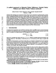
Average volumetric percentages of additives used for horizontal drilling and hydraulic fracturing in multiple oil and gas plays. See §1.1.2. Source: FracFocus (2012). . . . . . . . . . . . . . . . . . . .

1.2

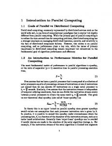
3

Conceptualization of the process of Carbon Capture, Utilization, and Sequestration (§1.1.1) highlighting active research areas. See §1.1.3. Source: NETL (2011). . . . . . . . . . . . . . . . . . . . . .

2.1

4

A one-dimensional uniform nodal grid with (m + 1) nodes and stepsize ∆x = 0.5. This figure depicts how the approximations for a discrete gradient are bound to the grid, as well as the importance of the boundary nodes. See §2.2.3.

2.2

. . . . . . . . . . . . . . . . . . 22

A two-dimensional uniform nodal grid with 5 × 5 nodes and stepsizes ∆x = ∆y = 0.25. See §2.2.3. . . . . . . . . . . . . . . . . . . . 23

2.3

A one-dimensional uniform staggered grid with m cells, (m + 1) nodes, and step-size ∆x = 0.5. This figure depicts how the approximations for the discrete gradient and divergence are bound to the staggered grid. See §2.2.3. . . . . . . . . . . . . . . . . . . . . . . . 24

2.4

A one-dimensional uniform staggered grid with m cells, (m + 1) nodes, and step-size ∆x = 0.5. This figure depicts how the approximations for a discrete Laplacian are bound to the staggered grid. See §2.2.3. . . . . . . . . . . . . . . . . . . . . . . . . . . . . . . . . 24

2.5

A two-dimensional uniform staggered grid with step-sizes ∆x and ∆y. This figure depicts how the approximations for the discrete Laplacian are bound to the staggered grid, in analogy to the onedimensional case. See §2.2.3. . . . . . . . . . . . . . . . . . . . . . . 25

2.6

A one-dimensional uniform staggered grid with 5 cells, 6 nodes, and step-size ∆x = 0.5. Visualized using the package developed by Sanchez (2015a). See §2.2.3. . . . . . . . . . . . . . . . . . . . . . . 26

xxiii

List of Figures 2.7

xxiv

A two-dimensional uniform staggered grid with 5 × 6 cells, each with its own center, with step-sizes ∆x = 0.5 and ∆y = 0.1667. Visualized using the package developed by Sanchez (2015b). See §2.2.3. . . . . . . . . . . . . . . . . . . . . . . . . . . . . . . . . . . 26

2.8

A three-dimensional uniform staggered grid with 5×6×7 cells, each with its own center, with step-sizes ∆x = 0.5, ∆y = 0.1667, and ∆z = 0.1429. Visualized using the package developed by Sanchez (2015c). See §2.2.3. . . . . . . . . . . . . . . . . . . . . . . . . . . . 27

3.1

Proposed modification to the Castillo–Runyan–Sanchez Algorithm yielding the proposed CBS Algorithm. See §3.4. . . . . . . . . . . . 60

3.2

Computed value of the weights according to the selected objective function. For this figure, an eight-order divergence was built. We also plot the average of all of the values, and the values using the CRS algorithm. It can be seen that q4 is negative for this case, but through the CBS algorithm is then made equal to . See §3.5.1. . . 66

4.1

The natural lexicographical order, as mapped to both the sets of arguments and the set of results of the 2D mimetic operators. See

4.2

Figure 2.4 in §2.2.3. See §4.1. . . . . . . . . . . . . . . . . . . . . . 72 ˘ k . In ˘ k , and L ˘k , D Attained matrices implementing operators G xy xy xy this example, a domain with 5 cells per dimension is used. nz

4.3

denotes the number of non-zero elements. See §4.1. . . . . . . . . . 74 ˘k , D ˘ k , and L ˘k . Attained matrices implementing operators G xyz xyz xyz In this example, a domain with 5 cells per dimension is used. nz denotes the number of non-zero elements. See §4.2. . . . . . . . . . 76

4.4

Solutions for the test case. In this example, a domain with 5 cells

4.5

per dimension has been defined. See §4.3. . . . . . . . . . . . . . . . 77 ˘ k operator. In this example, Attained matrices implementing the L xy

a domain with 5 cells per dimension has been defined. See §4.1. . . 78 4.6

An intuitive depiction of the mathematical interpretation of the curl operator. See §4.4. . . . . . . . . . . . . . . . . . . . . . . . . . . . 79

4.7

A small rotating disk S, bounded by C, with an orienting normal n. A limiting process then takes place by collapsing the diameter of S to 0, thus allowing for a definition for the curl operator based on Stokian circulation. See §4.4. . . . . . . . . . . . . . . . . . . . . 80

List of Figures 4.8

xxv

A limiting process for an infinitesimally thin disk S with boundary C and orienting normal n created upon collapsing surfaces Su and Sd , aligned through a mantle M of width w, which is then considered to tend to 0. See §4.4. . . . . . . . . . . . . . . . . . . . . . . . . . 81

4.9

A Gaussian-like flux, through the infinitesimally thin disk S. See §4.4. . . . . . . . . . . . . . . . . . . . . . . . . . . . . . . . . . . . 83

4.10 The auxiliary vector fields acting on a 2D domain implicitly define a translation of the grid, thus making up for the interpolation of the original method proposed in Runyan (2011). See §4.4. Source: Castillo and Miranda (2013). . . . . . . . . . . . . . . . . . . . . . . 85 4.11 The auxiliary vector fields acting on a 3D domain implicitly define a translation of the grid, thus making up for the interpolation of the original method proposed in Runyan (2011). See §4.4. Source: Castillo and Miranda (2013). . . . . . . . . . . . . . . . . . . . . . . 86 4.12 A detailed depiction of two out of three auxiliary fields on a cell of the auxiliary grid, discretizing a 3D vector field. See §4.4. . . . . . . 87 4.13 Actual computation of the 3D curl and its binding to the implicitly defined auxiliary staggering. See §4.4. . . . . . . . . . . . . . . . . . 87 4.14 Vector field: v(x) = −yi + xj. See §4.4. . . . . . . . . . . . . . . . . 88 4.15 Known curl field: ∇ × v = 2k. See §4.4. . . . . . . . . . . . . . . . 88 4.16 A 2D discretization of the proposed vector field, on a logically rect˘2 . angular 2D uniform staggered grid, to test the correctness of D xy

See §4.4. . . . . . . . . . . . . . . . . . . . . . . . . . . . . . . . . . 89 ˘ 2 . See §4.4. . . . . . . . . . . . . . . . . . . . 90 4.17 Result of applying D xy ∗ = v × k. See §4.4. . . . . . . . . . . . . . 90 4.18 Auxiliary vector field: vxy

4.19 Computed mimetic curl (Gaussian). See §4.4. . . . . . . . . . . . . 91 4.20 A velocity field v1 described by a counterclockwise vortex flow. See §4.4. . . . . . . . . . . . . . . . . . . . . . . . . . . . . . . . . . . . 91 4.21 A velocity field v2 described by a uniform sink flow. See §4.4. . . . 92 4.22 A hurricane model that combines a velocity field (counterclockwise vortex flow) around a chosen reference point (e.g. the origin) of strength k, v1 (x, y), and a uniform sink flow toward the reference point of strength q, v2 (x, y). See §4.4. . . . . . . . . . . . . . . . . . 93 4.23 Computed divergence of the hurricane model, i.e. ∇ · h. See §4.4. . 94

List of Figures

xxvi

4.24 Computed curl of the hurricane model, which allows then to numerically compute the vorticity as Γ = 2||∇ × h||, across the given domain. See §4.4. . . . . . . . . . . . . . . . . . . . . . . . . . . . . 94 5.1

UML class diagram modeling of a 1D grid and its nodes. For layout purposes, we do not render the full name of the class. See §5.1. . . . 100

5.2

Summary of the MTK Concerns (architecture of the MTK), showing the existing interdependence among layers. See §5.3.

5.3

. . . . . . . . 105

Elided UML class diagram for data-structures in the MTK’s “Data structures” concern (second layer) (see Figure 5.2). See §5.3.2. . . . 108

5.4

Elided UML class diagram for the implemented grid-related mechanisms within the MTK’s “Meshes and grids” concern, located in the third layer (see Figure 5.2). See §5.3.2. . . . . . . . . . . . . . . 109

5.5

Elided UML class diagram for the modeling of mimetic operators. See §5.3.3. . . . . . . . . . . . . . . . . . . . . . . . . . . . . . . . . 109

5.6

Known analytical solution for example problem number one. A uniform nodal grid with 102 cells was used to generate this plot. See §5.4.1. . . . . . . . . . . . . . . . . . . . . . . . . . . . . . . . . 111

5.7

Computed numerical solution for sample problem one, using a onedimensional uniform staggered grid with only 5 cells (Figure (a)) and 102 cells (Figure (b)), as well as second-order mimetic operators. Figure (a) shows how is the Laplacian bound to the centers of the cells in the numerical solution, as it can be seen in Figure 2.4. See §5.4.1. . . . . . . . . . . . . . . . . . . . . . . . . . . . . . . . . 113

5.8

Solution through the MTK to the problem in §5.4.2. A Cr = 1 was considered for this case. See §5.4.2. . . . . . . . . . . . . . . . . . . 114

5.9

Snapshots for the problem described in §5.4.3. For this example, we used 50 cells per spatial coordinate. These snapshots were attained thanks to the MMTK. See §5.4.3. . . . . . . . . . . . . . . . . . . . 117

6.1

Summary of the major compositional divisions of planet Earth, as a function of depth. See §6.1. Source: Adapted from information given by Walther (2009). . . . . . . . . . . . . . . . . . . . . . . . . 120

6.2

p − T diagram for CO2 . See §6.2. Source: Created from models given by Marini (2006a). . . . . . . . . . . . . . . . . . . . . . . . . 121

6.3

Schematics of the algorithmics of WebSym.C present at the numerical core called Sym.8. See §6.3. Source: Park (2009). . . . . . . . . 125

List of Figures 6.4

xxvii

Solutions at five years, computed in blackbox.sdsu.edu. We compute concentration of CO2 , H+ , and Fe++ , as a function of distance from the injection well. See §6.6. . . . . . . . . . . . . . . . . . . . 129

7.1

Highest ten percentages of invested computation time (in seconds) per routine in the original version of WebSym.C , as computed by GNU gprof in blackbox.sdsu.edu. See Table 7.1. The average of five instances of on hundred cells each of the pilot test case described in §6.5 was considered for this profiling study. See §7.1. . . . . . . . 133

7.2

Results of tests performed by ATLAS in order to inquire about attained performance in the development architecture. Tests consist of executing certain kernel routines and reporting performance as a percentage of clock rate. See §7.2. . . . . . . . . . . . . . . . . . . . 134

7.3

Behavior of the rank of the BloGS matrices, as a function of the number of solutes Na and the number of nodes, nx . Coloring is simply a result of the plotting software used; it means nothing special except that is varies proportionally to the quantity of being plotted. See §7.3. . . . . . . . . . . . . . . . . . . . . . . . . . . . . . . . . . 137

7.4

Bandwidth and (absolute) density of the BloGS matrices, which are properties that depend on the chosen order of accuracy, ω. Coloring is simply a result of the plotting software used; it means nothing special except that is varies proportionally to the quantity of being plotted. See §7.3. . . . . . . . . . . . . . . . . . . . . . . . . . . . . 140

7.5

Projections depicting the behavior of the important properties of a BloGS matrix. Coloring means nothing. See §7.3. . . . . . . . . . . 141

7.6

R R2008a prototype driver for Attained results for the MATLAB

the solution of a BloGS system. See §7.3.2. . . . . . . . . . . . . . . 144 7.7

Behavior of the condition number of the BloGS matrices, as a function of the rank r(nx ), which is defined by the number of nodes, nx . See §7.3. . . . . . . . . . . . . . . . . . . . . . . . . . . . . . . . . . 145

7.8

Analytical and computed solutions for the prototype drivers implemented using the LAPACK and SuperLU SEQ , for the solution of a BloGS system. Coloring distinguishes the analytical and computed solution. Specifically, dots depict the computed solution whereas the line connecting the hollow circles depict the analytical solution. See §7.3.2. . . . . . . . . . . . . . . . . . . . . . . . . . . . . . . . . 146

List of Figures 7.9

xxviii

Analytical and computed solutions for the prototype drivers developed using the LAPACK and SuperLU SEQ for the solution of a BloGS system. p stands for number of processing cores. See §7.3.3. 148

7.10 Attained qualities for the speedup under a more comprehensive (r, β)-space (rank and bandwidth). See Tables 7.4 and 7.5. Coloring is simply a result of the plotting software used; it means nothing special except that it is useful to visualize differentiate the different collection of values being plotted. See §7.3.3. . . . . . . . . . . . . . 151 8.1

Naturally occurring ground-level sandstone sedimentary systems. See §8.1. Source: Author’s personal collection. . . . . . . . . . . . . 154

8.2

Proposed simulation scenario for a mimetic mass transport simulation driver. See §8.1. . . . . . . . . . . . . . . . . . . . . . . . . . . 154

8.3

Proposed simulation scenario for a mimetic mass transport simulation driver. Discretization of the domain of interest using a 2D uniform staggered grid. The grid was rendered using the package developed by Sanchez (2015b). See §1.1.2. . . . . . . . . . . . . . . 155

8.4

Proposed options to model the initial concentration in the reservoir. See §7.3.3. . . . . . . . . . . . . . . . . . . . . . . . . . . . . . . . . 158

8.5

Architectural details of the platform where the results were attained. This figure was generated with the hwloc utility. See §8.4. . . . . . . . . . . . . . . . . . . . . . . . . . . . . . . . . . . . . . . 159

8.6

Software collection and its data management plan. The MMTK and the MTK are both known as flavors in this image, since they are part of a broader collection to be discussed in Chapter 9. See §8.4. . . . . . . . . . . . . . . . . . . . . . . . . . . . . . . . . . . . 159

8.7

Example of a 2D uniform staggered grid for the discretization of the domain of interest. Rendered using the package developed by Sanchez (2015b). See §8.4. . . . . . . . . . . . . . . . . . . . . . . . 160

8.8

Effect of computing the first time-step before the introduction of the second-order stage. See §8.4. . . . . . . . . . . . . . . . . . . . . 161

8.9

Diffusion of carbon dioxide, one month after injection. See §8.4. . . 161

8.10 Concentration profiles under the diffusive-advective model at 48 hours after injection, using different initial conditions. See §7.3.3. . 163 8.11 Concentration profiles under the diffusive-advective model at 48 hours after injection, using a gradient-based initial condition, in the context of the proposed simulation scenario. See §7.3.3. . . . . . 164

List of Tables 3

Notational conventions adopted in this work. . . . . . . . . . . . . . xli

2.1

A summary of algorithmic schemes arising from numerically solving any given Initial/Boundary Value Problem. See §2.2.2. . . . . . . . 21

2.2

A summary of how are the discrete operators computed in 1, 2, and 3D. We summarize how are the results bound to the respective staggered grid. See §2.2.3. . . . . . . . . . . . . . . . . . . . . . . . 26

2.3

A summary of how are the discrete operators computed in 1, 2, and 3D. We summarize how are the arguments these take bound to the respective staggered grid. See §2.2.3. . . . . . . . . . . . . . . . . . 26

3.1

Attained values for the weights as a function of the chosen row to be the objective function. In this implementation, the positivedefiniteness constraint was not requested. Therefore, for any selected row, we obtained the same values as both the CRM and the CGM, thus showing the validity of the CLO-based algorithm, to construct mimetic divergence operators. See §3.5. . . . . . . . . . . 65

3.2

Attained values for the weights as a function of the chosen row to be the objective function. In this implementation, the weight vector was not initialized to zero, before selecting a different row to resolve the CLO problem. See §3.5. . . . . . . . . . . . . . . . . . . . . . . 65

3.3

Results of the CBS algorithm versus the CRS algorithm in higher orders. For this second set of results, an 8th-order mimetic divergence was constructed and a default value of = 1.00E-06 was considered. See §3.5.1. . . . . . . . . . . . . . . . . . . . . . . . . . 67

xxix

List of Tables 3.4

xxx

Computed weights according to the selected objective function. These results were computed for an 8th-order divergence, which is the lower order for which the problem of negative weights appears, when constructing a divergence operator. We compute the relative error on norm 2 with respect to the solution taken when the constraint gets turned off. This is taken as the exact solution satisfying the extended form of Gauss’ Divergence Theorem, presented in Equation (2.31). For this set of results, a default value of = 1.00E-06 was used. See §3.5.1. . . . . . . . . . . . . . . . . . . . 69

3.5

Computed weights according to the selected objective function. These results were computed for an 10th-order gradient, which is the lower order for which the problem of negative weights appears, when constructing a gradient operator. We compute the relative error on norm 2 with respect to the solution taken when the constraint gets turned off. This is taken as the exact solution satisfying the extended form of Gauss’ Divergence Theorem, presented in Equation (2.31). For this set of results, a default value of = 1.00E-06 was used. See §3.5.1. . . . . . . . . . . . . . . . . . . . . . . . . . . 70

5.1

Summary of possible multiplicities when modeling in the UML. See §5.1. . . . . . . . . . . . . . . . . . . . . . . . . . . . . . . . . . . . 102

5.2

Calculation of the attained error using MTK objects for the entire grid. See §5.4.1. . . . . . . . . . . . . . . . . . . . . . . . . . . . . . 113

5.3

Calculation of the attained error using MTK objects for the west and east boundaries. See §5.4.1. . . . . . . . . . . . . . . . . . . . . 114

6.1

Comparison of considered hardware platforms in terms of performance characteristics. See §6.6. . . . . . . . . . . . . . . . . . . . . 128

7.1

Top ten percentages of invested computation time (in seconds) per routine in WebSym.C, as computed by GNU gprof Fenlason (1993) in blackbox.sdsu.edu. See Figure 7.1. The average of 5 instances of 100 cells each of the pilot test case described in §6.5 was considered for this profiling study. See §7.1. . . . . . . . . . . . . . . . . . 132

7.2

Attained execution times (in minutes) from replacing the reference sequential solver with those discussed in §7.2. The averages of 5 executions were taken per each case. See §7.2. . . . . . . . . . . . . 134

7.3

Comparison of selected solvers to work with. See §7.3.3. . . . . . . . 146

List of Tables

xxxi

7.4

Attained qualities for low-rank matrices. See Figure 7.10a. See §7.3.3.149

7.5

Attained qualities for high-rank matrices. See Figure 7.10b. See §7.3.3. . . . . . . . . . . . . . . . . . . . . . . . . . . . . . . . . . . 149

7.6

Execution times (in seconds) for the proposed test case using SuperLU DIST on blackbox.sdsu.edu. See §7.3.3. . . . . . . . . . . 150

7.7

Execution times using ScaLAPACK on blackbox.sdsu.edu. Reported in seconds. See §7.3.3. . . . . . . . . . . . . . . . . . . . . . 150

List of Algorithms

1

The Castillo–Runyan–Sanchez Algorithm to construct k-th order (k even and positive) mimetic gradient and divergence operators. Part 1: Interior of the grid. See §3.2.1. . . . . . . . . . . . . . . . . . . . . 38

2

The Castillo–Runyan–Sanchez Algorithm to construct k-th order (k even and positive) mimetic divergence operators. Part 2.1: Boundary points: preliminary steps. See §3.2.2. . . . . . . . . . . . . . . . . 40

3

The Castillo–Runyan–Sanchez Algorithm to construct k-th order (k even and positive) mimetic divergence operators. Part 2.2: Boundary points: null-space columns and approximating columns of the Π matrix to compute the weights. See §3.2.2. . . . . . . . . . . . . . . . 43

4

The Castillo–Runyan–Sanchez Algorithm to construct k-th order (k even and positive) mimetic divergence operators. Part 2.3.i: Boundary points: creation of the Π matrix to compute the weights of the divergence operator. See §3.2.2. . . . . . . . . . . . . . . . . 45

5

The Castillo–Runyan–Sanchez Algorithm to construct k-th order (k even and positive) mimetic gradient operators. Part 2.3.ii: Boundary points: creation of the Π matrix to compute the weights of the gradient operator. See §3.2.2. . . . . . . . . . . . . . . . . . . . . . 46

6

The Castillo–Runyan–Sanchez Algorithm to construct k-th order (k even and positive) mimetic divergence operators. Part 2.4: Boundary points: computing the weights using the Π matrix. See §3.2.2. . 49

7

The Castillo–Runyan–Sanchez Algorithm to construct k-th order (k even and positive) mimetic divergence operators. Part 3: Assembling the final matrix operator. See §3.2.3 . . . . . . . . . . . . . . . 50 xxxiii

List of Algorithms 8

xxxiv

The Castillo–Blomgren–Sanchez Algorithm to construct k-th order (k even and positive) mimetic divergence operators. Part 2.3.i: ˜ matrix to compute the weights of the operator. Construction of the Π See §3.4. . . . . . . . . . . . . . . . . . . . . . . . . . . . . . . . . . . 58

9

The Castillo–Blomgren–Sanchez Algorithm to construct k-th order (k even and positive) mimetic divergence operators. Part 3: Construction of the system to be solved as a Constrained Linear Optimization problem. See §3.4. . . . . . . . . . . . . . . . . . . . . . . . 62

10

A C++ programming interface to implement the construction of a mimetic 1D gradient. The CBS Algorithm is implemented as the constructor the class. C++ polymorphism (see Chapter 5) allows for the existence of two constructors. One assuming a default mimetic threshold of = 1.00E-06, and another that allows developers to specify it. See §3.5. . . . . . . . . . . . . . . . . . . . . . . . . . . . . 63

11

A C++ programming interface to implement the construction of a mimetic 1D divergence. The CBS Algorithm is implemented as the constructor the class. C++ polymorphism (see Chapter 5) allows for the existence of two constructors. One assuming a default mimetic threshold of = 1.00E-06, and another that allows developers to specify it. See §3.5. . . . . . . . . . . . . . . . . . . . . . . . . . . . . 64

Abbreviations and Acronyms GHG

Greenhouse Gas

USA

United States (of) America

EPA

Environmental Protection Agency

CCUS

Carbon Capture, Utilization, (and) Sequestration

EOR

Enhanced Oil Recovery

EGR

Enhanced Gas Recovery

MTK

Mimetic Methods Toolkit

CSRC

Computational Science Research Center

SDSU

San Diego State University

OpenMP

Open Multi-Processing

MPI

Message Passing Interface

SFDs

Standard Finite Differences

ODEs

Ordinary Differential Equations

PDEs

Partial Differential Equations

IC

Initial Condition

BC

Boundary Condition

IBVP

Initial/Boundary Value Problem

BTCS

Backward (in) Time (and) Central (in) Space

MFDs

Mimetic Finite Differences

CGM

Castillo–Grone Method

CRM

Castillo–Runyan Method

CLO

Constrained Linear Optimization

CRS

Castillo–Runyan–Sanchez xxxv

Abbreviations and Acronyms

xxxvi

RHS

Right-Hand Side

CBS

Castillo–Blomgren–Sanchez

GLPK

GNU Linear Programming Kit

GNU

GNU’s Not Unix!

ADT

Abstract Data Type

OOP

Oject-Oriented Programming

UML

Unified Modeling Language

API

Applications Programming Interface

LST

Lyskov Substitution Principle

CRS

Compressed Row(-wise) Storage

CCS

Compressed Column(-wise) Storage

DOK

Dictionary of Keys

MMTK

MATLAB (wrappers for the )Mimetic Methods Toolkit

XSEDE

Extreme Science (and) Engineering Discovery Environment

SDSC

San Diego Supercomputing Center

BloGS

Block-Defined, Global, and Sparse

LAPACK

Linear Algebra PACKage

ATLAS

Atumatically Tuned Linear Software

Physical Constants Acceleration due to the gravitational field

xxxvii

g

=

9.80665 m/s2 .

Notational Conventions 1. We shall denote both integer and continuous scalar-valued quantities, say rank of a matrix, temperature, or pressure, with the default math pseudoitalicized font, and using combinations of both lower and uppercase Latin letters and lowercase Greek letters: a, ..., z, A, ...Z, α, ..., ω. Discretized instances shall be identified with a tilde accent, and will be assumed to be computationally implemented as row-wise-defined arrays, except when otherwise noticed. 2. We shall denote continuous vector-valued quantities using boldfaced lowercase Latin letters: a, ..., z. Discretized instances shall be identified with a tilde accent, and will be assumed to be computationally implemented as row-wise-defined arrays, except when otherwise noticed. The vectors on the ˆ canonical Euclidean base will be denoted as î, ˆj, and k. 3. We shall denote matrices using boldfaced uppercase Latin and Greek letters: A, ..., Z, Γ, ..., Ω. 4. We shall denote continuous tensor-valued quantities using scripture-styled uppercase Latin letters: A , ..., Z . Discretized instances shall be identified with a tilde accent. 5. We shall denote continuous differential operators using standard notation from Calculus. When it comes to their discrete matrix analog operators, we will use boldfaced uppercase Latin Letters with a tilde accent, thus emphasizing the approximation to a continuous operator they intend to. However, those operators built by means of the Castillo–Grone or the Castillo–Runyan xxxix


xl

Mimetic Finite Difference Method, through any of the algorithms discussed in this work, shall be identified with a breve accent. As a side note, this notational convention is supported by the fact that, on German cartography, a breve accent placed over two letters is often used in abbreviated place names ˘ as a short for “burg”, a common suffix originally meaning that end in “bg”, “Castle”, which is English for “Castillo”. This prevents misinterpretation since “berg” is another common suffix in place names, which means “moun˘ stands for “Freiburg”, not “Freiberg”. tain”. Thus, for example, “Frei bg” Furthermore, its is also mnemonic, since it resembles a letter ‘C’. 6. In this work, mimetic operators are built using matrix notation, yet two aspects are important enough to deserve their own notational convention: their order of accuracy and their dimensionality. Based on this, we will denote a k-th order-accurate (k even and positive), on the (x, y, z), (x, y), or x rectangular domains (3, 2 or 1D), mimetic operator as: ˘k (a) Mimetic gradient: G {xyz,xy,x} . ˘k (b) Mimetic divergence: D {xyz,xy,x} . ˘k (c) Mimetic Laplacian: L {xyz,xy,x} . ˘k (d) Mimetic curl: C {xyz,xy,x} . 7. We shall denote sets using italic uppercase Greek letters: A, ..., Ω. Discretized instances shall be identified with a tilde accent, and will be assumed to be computationally implemented as row-wise-defined arrays, except when otherwise noticed. 8. Numerical sets will be denoted with blackboard boldfaced Latin uppercase letters: A, ..., Z. 9. Chemical species for which to keep track of their phase is important will be subscripted using the following symbols: {so, li, ga, sc}, which denote solid, liquid, gaseous, and supercritical phase, respectively.


xli

Table 3: Notational conventions adopted in this work. Object Scalar Vector Matrix Tensor Operator Set

Continuous domain a, ..., z, A, ...Z, α, ..., ω a, ..., z A, ..., Z, Γ, ..., Ω A , ..., Z ∇, ∇·,... A, ..., Ω or A, ..., Z

Discrete domain ˜ ..., Z, ˜ α a ˜, ..., z˜, A, ˜ , ..., ω ˜ ˜, ..., z ˜ a A, ..., Z, Γ, ..., Ω A˜, ..., Z˜ ˜ ˜ or A, ˘ ..., Z ˘ A, ..., Z ˜ ..., Ω ˜ A,

Indexed ai , ..., zi , Ai , ...Zi , αi , ..., ωi ai , ..., zi aij , ..., zij , αij , ..., ωij Aij , ..., Zij A˜ij , ..., Z˜ij or A˘ij , ..., Z˘ij ˜i A˜i , ..., Ω

R 16, 10. All of the algorithms in this work were originally designed in Maple

thus the notation and the names for the functions selected for the pseudocodes. It is noteworthy that we are not assuming the interested reader R 16 in order to test these algorithms; we are just using requires Maple

Maple’s notational conventions for pseudo-code.

Table 3 summarizes our notational conventions. An important thing to notice is that, when accessed by means of indexing the elements they may contain, the objects shall not conserve their typographical style, thus yielding a default math pseudo-italicized font. For example, notice that tensors loose their typographical style, in this case, their scripture style, thus yielding a default math pseudoitalicized font uppercase Latin letter. This can be depicted in columns three and four of Table 3. However, when objects are indexed as being part of a enumerable set, they will preserve their typographical style.

Chapter 1 Introduction

1.1

Context of This Work

Nowadays, the production of electrical energy is an important challenge. Different production methods exist, and they differ in usage of resources and in interaction with the environment. Based on these differences, these methods can be classified according to an important dichotomy that has been imposed, as a matter of course. Production methods can be classified as green energy production methods or gray energy production methods. Green energy production methods comprise production technologies based on renewable natural resources. Examples include solar, eolic, hydrological, and geothermal energy production, among others. These methods characterize themselves for having an efficient interaction with the environment. This means that the anthropogenic impact of implementing these methods is relatively low. However, renewable natural resources depend largely on geographical features and climatological conditions. Thus, they are not as reliable as their gray counterparts. Gray energy production methods comprise production technologies based on naturally occurring fossil fuels, such as oil, natural gas, or coal. These methods are often more reliable than green methods, since they rely on resources that are naturally abundant. However, their environmental impact is stronger than that of 1

2 — Chapter 1: Introduction

By Eduardo J. Sanchez

green methods. This is because, for example, greenhouse gas (GHG) emissions stem from burning fossil fuels (EPA, 2012a). The steady accumulation of GHGs from the combustion of fossil fuels has led to an increase in the amount of solar radiation trapped between the atmosphere and the Earth (Shakun, 2012). This increased radiation raises the temperature of the Earth’s atmosphere and ocean systems. Many researchers believe that this continuing increment in temperature will lead to catastrophic changes in weather conditions around the globe (White et al., 2003). Therefore, with carbon dioxide (CO2 ) being the most abundant GHG, many efforts are underway to reduce the levels of CO2 entering the atmosphere. For example, in April of 2012, the United States of America (USA) Environmental Protection Agency (EPA) proposed a regulatory legislative framework to limit GHG emissions from new fossil fuel-fired power plants by limiting CO2 emissions (see EPA, 2012b).

1.1.1

Carbon Capture, Utilization, and Sequestration

Carbon capture, utilization, and sequestration (CCUS) is a collection of technologies that intend to mitigate the environmental impact of GHGs arising from the combustion of fossil fuels. Specifically, these technologies seek to first separate and capture the CO2 from flue gases expelled by coal-fired power plants. The collected CO2 is then transported (if required) to the injection site, where it is compressed to above its critical pressure. As it is injected into underground formations, such as depleted oil reservoirs, gas reservoirs, or deep brine aquifers, the geothermal gradient heats the CO2 to above its critical temperature, thus taking it to a supercritical phase (CO2(sc) ) (see White et al., 2003). Once in the underground reservoir, the CO2 can be utilized for further purposes. An example of CO2 utilization, which is key for the financial appeal of CCUS, is established by the assortment of Enhanced Oil/Gas Recovery (EOR/EGR) methods in hydrocarbons extraction (see Ewing, 1983).

Ph.D. Thesis in Computational Science

San Diego State University, 2015

Chapter 1: Introduction

By Eduardo J. Sanchez — 3

Several methodologies for the extraction of hydrocarbons trapped in sandstone formations have been broadly studied and implemented thus far. Unfortunately, most of these techniques are still not very effective, so significant amounts of hydrocarbons often remain in the reservoir (50% or more). In order to recover more of the residual hydrocarbons, several EOR methods involving complex chemical and thermal effects have been developed.

Figure 1.1: Average volumetric percentages of additives used for horizontal drilling and hydraulic fracturing in multiple oil and gas plays. See §1.1.2. Source: FracFocus (2012).

One method for EOR is based on the injection of gases, such as CO2 , which mix with the resident hydrocarbons, forming a single fluid phase. This makes complete hydrocarbon recovery possible, since the miscible phase flows more readily than the oil (see Ewing, 1983). Once properly utilized (if so), the CO2 is to remain sequestered in the chosen underground formation. The success of the sequestration is then estimated by means of constant surface-level monitoring efforts.

1.1.2

Horizontal Drilling and Hydraulic Fracturing

A different hydrocarbon extraction technique—often related to studies in CCUS— is called hydraulic fracturing, or fracking. Fracking aims to recover hydrocarbons trapped within the shale formations, rather than in sandstone formations. Ph.D. Thesis in Computational Science




Fracking profits from advances in shale horizontal drilling. Essentially, a horizontal well is drilled throughout the shale formation. Once the wellbore has been completed, exploding charges are placed, which crack the shale. Then, through hydraulic pumping, a mixture of approximately 99% water, silicate sand, and other chemicals (Figure 1.1) are injected into the fractured shale. The silicate sand helps the fractures to remain open. After this injected mixture is pumped back up the surface, the trapped hydrocarbons flow (due to the pressure gradient), from being trapped in the shale up to the surface.

Figure 1.2: Conceptualization of the process of Carbon Capture, Utilization, and Sequestration (§1.1.1) highlighting active research areas. See §1.1.3. Source: NETL (2011).

A crucial aspect for the success of the CCUS pipeline, is the efficient storage of CO2 in depleted sandstone oil reservoirs, or lithological traps. These are sedimentary rock formations in which the shale, or cap rock, traps the hydrocarbons present in the sandstone reservoir. Thus both fracking and CCUS benefit from studying fracture dynamics under pressure gradients. However, in this work, we will not study fracking, nor rock fracture mechanics. Ph.D. Thesis in Computational Science



1.1.3


The Importance of Simulating the Long-term Evolution of the Sequestered Carbon Dioxide

As mentioned, CCUS represents a promising alternative to help mitigate global warming. But, if significant amounts of CO2 are going to be sequestered in underground reservoirs, it is clear that the geochemical implications have to be analyzed. Figure 1.2 shows an schematic of the process of CCUS (explained in §1.1.1), in where the need for the study of the geochemical reactions following injection is depicted as an active research area (see NETL, 2011; Jun et al., 2013). An example of one important topic is the study of large-scale pressure build-ups in response to the injection, and how would they limit the storage capacity of suitable formations. Over-pressurization may fracture the caprock, thus causing leakage and induced seismicity (Zhou and Birkholzer, 2011; Song and Zhang, 2013). As mentioned in §1.1.2, this is a common concern for both fracking and CCUS, since the chance of leaking represents a significant risk (Harvey et al., 2013). A famous example is the disaster occurred on August 21, 1986, when roughly one cubic kilometer of gaseous CO2 escaped into the atmosphere from the floor of Lake Nyos in the hilly jungle terrain of western Africa. By sunrise, more than 1,700 people and 3,200 animals had died of asphyxiation (see Pentland, 2008). However, the benefits of CCUS make it hard to ignore, since it has been showed that power plants equipped with CCUS technology produce about 80% to 90% less CO2 than those without it. Also, CCUS could reduce the cost of climate stabilization by 30% (Pentland, 2008), and it is believed that CO2 can remain sequestered in such formations, depending on the chemical and mechanical characteristics of the underground resident water and rock constituents, for at least 1,000 years.




1.2


Problem Statement and Proposed Solution

In this work, we will study the evolution of the concentration of the injected CO2 , in order to analyze the potential for CO2 sequestration in time. Therefore, we will only be concerned with the sequestration stage of the CCUS process pipeline described in §1.1.1. We are interested in computing the long-term concentration profiles of injected CO2 in the subsurface. For this, we construct a mathematical model based on the conservation of mass equation. This triggers two problems that we will consider. First, the conservative nature of this equation forces us to consider discretization methods that provide conservative properties, while at the same time maintaining a good performance when it comes to numerical accuracy. We thus propose to study the theory and the performance of mimetic finite differences in solving for this model. We propose the design and development of a software library that encapsulates the theory of mimetic finite differences. We will call this library the Mimetic Methods Toolkit (MTK). Finally, we must analyze parallelization approaches that allow us to take advantage of solution methods for the solution of the systems of equation that arise from the problem discretization. We propose a matrix storage scheme to exploit the necessity of solving for multiple solutes, within a given geochemical system of interest.

1.3

Background of the Problem

Plenty of work is being done to understand every stage of the CCUS pipeline. For example, research on CO2 capture is addressed by Soong et al. (2012); Northington et al. (2012); Golombek et al. (2009), and research on numerical simulations can be found in the works of Zaman et al. (2012); Liu and Wilcox (2013), and Movagharnejad and Akbari (2011). For research on transport see the works of Ph.D. Thesis in Computational Science




Ji and Zhu (2013); McCoy and Rubin (2008), and ZEP (2011). For research in EOR/EGR methods see the works of Jaramillo et al. (2009); Suebsiri et al. (2006), and Khoo and Tan (2006). Finally, for research in post-injection CO2 monitoring see the works of Bao et al. (2013); Seto and McRae (2011), and McAlexander et al. (2011). Specific research in understanding the geochemistry of the sequestration stage is abundant. While Walther (2009) (for example) address general concerns, others, such as Marini (2006b), address the particular geochemistry modeling CO2 geologic sequestration scenarios. Practical problems address a diversity of issues. An example is that of estimating storage resources (see Hnottavange-Telleen et al., 2009), which implies the need for reservoir characterization techniques. These focus on subsurface mapping through different techniques. One example is the use of seismic wave propagation (see Sanchez, 2014). Reservoir characterization also focuses on evaluating trapping mechanisms (see Han et al., 2010). With respect to the injection site, risk assessment is vital. Different concerns arise. One of these concerns is CO2 plume migration, in order to analyze the longterm concentration of CO2 and related solutes, throughout the reservoir. Monitoring efforts, such as those described by Ringrose et al. (2009), Arts et al. (2008), and Chadwick et al. (2006), intend to assist in this task. But it is clear that, for the purpose of prediction, computational tools should yield a very clear and reliable perspective.

1.4

The Proposed Solution: State of the Art

Mathematical models that intend to simulate and to predict the long-term conservation of CO2 rely on the conservation of mass equation. Numerical models have been developed. For example the work of Juanes et al. (2010) intends to provide a numerical description of the problem of modeling subsurface mass transport.





Naturally, numerical models have evolved into simulation software that allows to simulate both the plume migration, as well as the related geochemical effects. Examples of these simulators are:

1. With over 30 years of continuous development, the ECLIPSE simulator, developed by Schlumberger, is the most feature-rich and comprehensive reservoir simulator on the market, covering the entire spectrum of reservoir models, including black oil, compositional, thermal finite-volume, and streamline simulation (see Schlumberger, 2014). 2. TOUGHREACT is a numerical simulation program for chemically reactive non-isothermal flows of multiphase fluids in porous and fractured media, developed by introducing reactive chemistry into the multiphase flow code TOUGH2 (see Lawrence Berkeley National Laboratory, 2014). 3. PFLOTRAN is an open source, state-of-the-art massively parallel subsurface flow and reactive transport code (see Lichtner et al., 2013). PFLOTRAN solves a system of generally nonlinear partial differential equations describing multiphase, multicomponent and multiscale reactive flow and transport in porous materials. Parallelization is achieved through domain decomposition using the PETSc (Portable Extensible Toolkit for Scientific Computation) libraries.

Most of the aforementioned applications are not open source, which prevents us from modifying the code to test for the performance of mimetic finite differences. Furthermore, given the restricted access to these implementations, code-wise, we can not understand how is the parallelization achieved. We will thus develop a prototype subsurface mass transport driver. The only exception is PFLOTRAN, but it is coded in Fortran 2003, and it heavily depends on libraries, which requires a lot of overhead. The reference existing simulator we will use in this work is called WebSym.C (see Paolini et al., 2011b). Ph.D. Thesis in Computational Science



1.5


Justification and Intellectual Impact of This Work

One of the tangible outputs of this work, the MTK, will provide the computational science community with an open-source toolkit for implementing mimetic finite differences. Scientific discovery will be advanced while promoting teaching, training, and learning by involving postdoctoral, graduate, and undergraduate students in the use of the MTK to develop new scientific applications that rely on mimetic discretization methods.. Because the MTK is designed as a portable library, using an object-oriented design methodology, complexity underlying the creation of mimetic approximations will be encapsulated, which allows students to focus more on applying mimetic finite differences to their respective research problems. Furthermore, the MTK will provide a unifying software framework within which students can study the theory of mimetic finite differences. Teaching using the MTK will contribute to interdisciplinary learning, since students will need to understand the mathematics governing a problem, the theory of mimetic finite differences, and programming techniques required to use the library in a software project. The produced subsurface mass transport driver will be integrated into SubFlow, an object-oriented, high-performance simulation environment, currently being developed at the Computational Science Research Center (CSRC), at San Diego State University (SDSU). This driver will implement mimetic finite differences through the MTK, which will consolidate the research on mimetic finite differences to the study of the geochemistry of subsurface mass transport. Finally, this work has yielded several publications so far, thus contributing towards advancing research on several scientific communities. Research on the fields of numerical methods enjoys the contributions on developing and clarifying the theory of mimetic finite differences. The alpha version of the MTK has been fully explained by Castillo and Miranda (2013); Sanchez et al. (2012) and Sanchez et al. (2014b). The work presented by Sanchez et al. (2015b) explains the construction Ph.D. Thesis in Computational Science




of higher-order mimetic operators, through a novel method based on constrained linear optimization. Finally, research on parallelization schemes for subsurface mass transport problems, has been published by Sanchez et al. (2014a).

1.6

Objectives and Scope of This Work

The proposed research project has the following general objective:

To explore the role of mimetic finite difference techniques, and of parallel computing tools to achieve the solution to a mass transport problem on porous media, modeling the Earth’s subsurface, to inquire regarding the implications of the long-term geologic sequestration CO2 . The specific objectives are:

1. To study and develop the theory of mimetic finite differences, so that we can propose an algorithm to construct 1D mimetic approximations, for any given order of numerical accuracy. 2. The extend the proposed algorithm to construct higher-order mimetic approximations in higher-dimensions. 3. To study and develop the theory for a parallelization scheme that exploits the physical nature of the problem of geochemical concentration profiles computations. 4. To implement all of these related results into the MTK. This includes to develop the library’s architecture, and its data management plan. 5. To construct a prototype driver code implementing a mimetic solution, for a 1D, seconds-order accurate, diffusion-reaction problem with multiple solutes, through the proposed parallelization scheme.





6. To construct a prototype driver code implementing a 2D mimetic solution a subsurface mass transport problem. 7. To study the potential for a parallel implementation of this problem, at the shared-memory level, through acceleration technologies, such as Open Multi-Processing (OpenMP) (The OpenMP Architecture Review Board, 2014). 8. To study the potential for a parallel implementation of this problem, at the distributed-memory level, through the use of the Message Passing Interface (MPI) (Barney, 2014).

1.7

Structure of This Document

This document is organized as follows: Chapter 1 presents the context of this work, as well as its justification and scope. Chapter 2 presents preliminary mathematical knowledge, which is important for this to be a self-contained work. Chapter 3 addresses the creation of higher-order 1D mimetic operators, as well as the details of their computational implementation. Chapter 4 then studies the construction of higher-dimensional mimetic operators, which use their 1D counterparts. Chapter 5 summarizes the theory on mimetic differential operators, and presents the design of the MTK. Chapter 6 presents a prime on the mathematical modeling, as well as the preliminary concepts, of subsurface mass transport. Preliminary simulations are also presented. Chapter 7 studies the computational performance of these simulations, and presents the mathematical development of a matrix storage scheme that allows for the computation of multiple solutes, in distributed-memory computers. Chapter 8 presents the details of a simulation driver implementing a mimetic discretization to solve for a subsurface mass transport problem. Ph.D. Thesis in Computational Science




Finally, Chapter 9 summarizes, concludes, and presents directions for future work.



Chapter 2 Mathematical Preliminaries In this chapter, in order for this to be a self-contained work, we introduce a few important mathematical concepts required to fully understand the material on the next chapters. We start with a quick review of our options when it comes to the numerical solution of linear systems of equations (§2.1). We then present a quick introduction to the key concept of differential operators. Specifically, we review important details of the continuous differential operators (§2.2.1). We then introduce their importance in describing physical models through partial differential equations, which allow us to naturally unveil the role of the discrete representation of these operators (§2.2.2). This discussion naturally leads to introducing important concepts related to space discretization through nodal and staggered grids (§2.2.3), on which we focus the first byproduct of this work; namely, a colR routines for grid visualization (§2.2.4). We conclude this lection of MATLAB

discussion with an introduction to mimetic differential operators (§2.3).

2.1

Solving Systems of Linear Equations

The solvability of the discrete problem attained when intending to numerically solve an IBVP is an important concern. For this, the singularity of the involved

13

14 — Chapter 2: Mathematical Preliminaries


matrix defining the arising system of equations is an important factor that is approached in the next definition: Definition 2.1. For a given non-singular matrix A, we define and denote its condition number as cond A , ||A|| · ||A−1 ||.

(2.1)

We note that cond A ≥ 1 and cond (γA) = cond A for any γ ∈ R. The second important consideration is how to solve the arising systems of equations. Systems of equations arise within many problems in science and engineering. Particularly, when numerically solving a linear PDE, we end up solving a system of linear equations Ax = b. Direct methods can be used if the size and data nature of the matrix are treatable, given the computational resources at hand. Instead, it is often necessary to use iterative methods. If the partial differential equation is nonlinear, then a nonlinear system of equations must be solved. In this work, we will study the solution to the arising systems of equations through Parallel Computing techniques.

2.2

Discrete Differential Operators

In this work, we are interested in the construction, properties, and application of discrete differential operators that mimic the properties of the continuum gradient, divergence, Laplacian, and curl differential operators. We will refer to these discrete operators as being mimetic; definition that shall be presented briefly.

2.2.1

Continuous Differential Operators

We recall the following definitions:



Chapter 2: Mathematical Preliminaries


Definition 2.2. Let f : R3 7−→ R be a scalar-valued field with continuous first partial derivatives on some open subset of R3 . We define and denote the (scalarevaluated, vector-valued) gradient field of f (x), in a Cartesian coordinates system, as: ∇f (x) ,

∂ ∂ ∂ ˆ f (x)î + f (x)ˆj + f (x)k, ∂x ∂y ∂z

(2.2)

ˆ are the elements of the canonical basis for R3 . where î, ˆj, k Definition 2.3. Let v : R3 7−→ R3 be a vector-valued field, defined as v(x) = ˆ We define and denote the (vector-evaluated, scalar-valued) p(x)î + q(x)ˆj + r(x)k. divergence field of v(x), in a Cartesian coordinates system, as: ∇ · v(x) ,

∂ ∂ ∂ p(x) + q(x) + r(x), ∂x ∂y ∂z

(2.3)

where p, q, r : R3 7−→ R have continuous first derivatives on some open subset of R3 . Definition 2.4. Let f : R3 7−→ R be a scalar-valued field with continuous first and second derivatives on some open subset of R3 . We define and denote the (scalarevaluated, scalar-valued) Laplacian field of f (x), in a Cartesian coordinates system, as: ∇2 f (x) ,

∂2 ∂2 ∂2 f (x) + f (x) + f (x). ∂x2 ∂y 2 ∂z 2

(2.4)

Recall that ∇2 f (x) = ∇ · ∇f (x). Definition 2.5. Let v : R3 7−→ R3 be a vector-valued field, defined as v(x) = ˆ We define and denote the (vector-evaluated, vector-valued) p(x)î + q(x)ˆj + r(x)k. curl field of v(x), in a Cartesian coordinates system, as: ∇ × v(x) ,

∂ ∂ ∂ ∂ ∂ ∂ ˆ r(x) − q(x) î + p(x) − r(x) ˆj + q(x) − p(x) k. ∂y ∂z ∂z ∂x ∂x ∂y (2.5)

where p, q, r : R3 7−→ R have continuous first derivatives on some open subset of R3 . Notational Remark For the sake of their computational implementation, we will agree on denoting: ∇ = grad, ∇· = div, ∇2 = lap, and ∇× = curl. Ph.D. Thesis in Computational Science




In this work, we study the discretization of continuous differential operators to compute the numerical solution of Ordinary and Partial Differential Equations (ODEs/PDEs). For a prime on the theory of ODEs/PDEs, consider the work of Hirsch et al. (2012) and Haberman (2003).

2.2.2

Standard Finite Differences and the Numerical Solution of Ordinary and Partial Differential Equations

The best known family of methods for the numerical solution of differential equations are the Standard Finite Differences (SFDs). These methods approximate the solutions to ODEs/PDEs using finite difference equations. These equations approximate the differential terms for time and space, with a certain order of numerical accuracy. We show this in the following example.

Example Let T be a measure of temperature. The heat equation for a homogeneous isotropic medium Ω states that: ∂T = κ∇2 T, ∂t

(2.6)

where κ , k/cp ρ is defined as the coefficient of thermal diffusivity, computed as a function of the medium’s coefficient of thermal conductivity k, its isobaric heat capacity cp , and its density ρ. Additionally, let T (t0 , x) = f (x) : Ω 7−→ R be a specified Initial Condition (IC), and let β(x) : ∂Ω 7−→ R be a specified Robin’s Boundary Condition (BC) (which can be periodic on ∂Ω) defined as: β(x) = δ(x)T (t, x) + η(x)(n · ∇T (t, x)),

(2.7)

where x ∈ ∂Ω, and:

1. δ(x) : ∂Ω 7−→ R is the Dirichlet Coefficient, 2. η(x) : ∂Ω 7−→ R is the Neumann Coefficient, and Ph.D. Thesis in Computational Science




3. n is the outward normal orienting the boundary ∂Ω.

For the sake of this example, let us consider a 1D rectangular domain, Ω := [a, b] ⊂ R, and κ = 1, leading to the following Initial/Boundary Value Problem (IBVP): ∂ 2T ∂T = ∂t ∂x2 T (t0 , x) = f (x)

(2.9)

δ(a)T (a) − η(a)∇T (a) = β(a)

(2.10)

δ(b)T (b) + η(b)∇T (b) = β(b)

(2.11)

(2.8)

By means of SFDs, there are many options to discretize the former PDE. Since this is a time-dependent problem, we must select a method to approximate both the temporal and the spatial component of the PDE. On SFDs, common combinations of selected difference equations are so familiar that they receive a name:

1. Selecting a first-order accurate forward difference equation for the temporal component, and a second-order accurate central difference equation for the spatial component, yields the forward in time and central in space (FTCS) method: i i Tji+1 − Tji Tj+1 − 2Tji + Tj−1 = . ∆t ∆x2

(2.12)

This is an explicit method, since we can solve for Tji+1 ; that is, the (i + 1)th time-step (or, (i + 1)-th snapshot) of the j-th space-step, yielding the following advancement equation for the method: Tji+1

∆t i ∆t ∆t i i = T + 1 − 2 T + T . j−1 j ∆x2 ∆x2 ∆x2 j+1

(2.13)

Here, ∆t, and ∆x denote the selected step-sizes for the discretization, and they yield m time-steps, and n space-steps, i.e., i ∈ [0, n], and j ∈ [0, m]. Ph.D. Thesis in Computational Science




Refer to Fornberg (1988) for a concise summary on how to derive the values for the approximating coefficients. Notational remark In this work, we will summarize ∆t and ∆x yielding m and n time-steps and spatial samples, respectively, using the familiar notation: i ∈ [0 : ∆t : tn ], and j ∈ [0 : ∆x : xm ]. When i = 0, we initialize the problem using its specified initial condition (see Equation (2.9)). Similarly, for T0i and Tmi , we use the specified boundary conditions, as in Equations (2.10) and (2.11). For this particular example, the FTCS explicit method is known to be numerically stable and convergent when: ∆t 1 ≤ . 2 ∆x 2

(2.14)

2. If we select instead a first-order accurate backward difference equation for the temporal component, we obtain the backward time, central space (BTCS) method: i+1 i+1 Tj+1 − 2Tji+1 + Tj−1 Tji+1 − Tji = . ∆t ∆x2

(2.15)

This is an implicit method, since we can not explicitly solve for the (i + 1)th snapshot, as in the FTCS Method. Instead, per each time-step, we must solve a system of linear equations: ∆t i+1 ∆t ∆t i+1 ∆t i − Tj−1 + 1 − 2 2 Tji+1 − Tj+1 = T . 2 2 ∆x ∆x ∆x ∆x2 j+1

(2.16)

The FTCS explicit method is always stable and convergent. 3. Finally, if we select a second-order accurate centered difference equation for the temporal component, and a second-order central difference equation for the spatial component at both time steps, we obtain the





Crank–Nicolson Method: Tji+1 − Tji 1 = ∆t 2

i+1 i+1 i i Tj+1 − 2Tji+1 + Tj−1 − 2Tji + Tj−1 Tj+1 + ∆x2 ∆x2

! .

(2.17)

The Crank–Nicolson Method is also an implicit method, since we must solve a system of linear equations in order to solve for the (i + 1)-th snapshot: i+1 i+1 i i , − rTj−1 + (2 − 2r)Tji + rTj+1 + (2 + 2r)Tji+1 − rTj+1 = rTj−1

(2.18)

where r,

∆t . 2∆x2

(2.19)

This method is also always stable and convergent. In fact, it is the most accurate scheme for small magnitudes of ∆t. The FTCS Method is the least accurate and can be unstable. The BTCS Method works the best for large magnitudes of ∆t.

Writing the discrete equations for SFDs methods using matrix notation unveils the role of discrete differential operators in a natural way. We can use matrix notation despite of the fact that we derive the finite difference equations through expansion of Taylor series, on scalar notation. Let us then consider the matrix form of the three methods introduced in the previous example. Let T˜ = [T0 , . . . , Tj , . . . , Tm ]> be an array of discretized temperature values to solve for, j ∈ [0, m] ⊂ R:





1. To describe the FTCS Method, consider the following discrete differential operator, defined from Equation (2.13), and described through a matrix:          ˜ F(r) ,       

δ(a)

0

···

···

0

0

r

(1 − 2r)

r

0

0

0

0

r

(1 − 2r)

r

0

0 ..

0



···

0

···

0

        .       

···

···

.

0

···

0

0

r

(1 − 2r)

r

0

0

···

0

0

0

r

(1 − 2r)

r

0

0

···

···

0

δ(b)

0

···

···

(2.20)

Notice that the first and last row are indeed comprised of nothing but zeros except for a couple of entrances. These rows act as placeholders for the discretization of the boundary conditions. In the case of Dirichlet’s Boundary Conditions, (for example) with Dirichlet coefficients δ(a) and δ(b) in the west and east, respectively, we will specify that F˜1,1 = δ(a), and F˜m,m = δ(b). Please refer to the work of LeVeque (2007) for the theoretical aspects of the construction of SFD-based discrete differential operators. For a prime of discrete differential operators based on Spectral Methods, consult the work of Trefethen (2000). Given the lower and upper bounds describing the discrete domain, selecting an adequate step-size yields a level of grid refinement. The resulting dimensions of the discrete operator are described through the number of nodes attained. For example, if we discretize throughout the x direction as ˜ x˜ = [0 : ∆x : xm ], then F(r) ∈ Rn×n . Based on the definition presented in Equation (2.20), we can then write Equation (2.13) as: ˜ T˜i . T˜i+1 = F(r)

(2.21)

Thus, the solution to a discretized PDE involves applying a discrete differential operator. In the case of Equation (2.21), the evolution in time is also discretized. This, being an explicit method, requires we initialize the discrete solution using a given initial condition, so that the future snapshot is Ph.D. Thesis in Computational Science




Table 2.1: A summary of algorithmic schemes arising from numerically solving any given Initial/Boundary Value Problem. See §2.2.2. Time influence

Type of method

Solution

Steady-state

Applying the discrete differential operator yields a system of equations due to considering specified BCs.

Time-dependent

Explicit

Initialize with a given IC and then, per each time step, apply a discrete differential operator considering specified BCs to get the next snapshot in time (solution at time (i + 1)). See Equation (2.21).

Time-dependent

Implicit

Initialize with a given IC and then, per each time step, applying the discrete differential operator yields a system of equations due to considering specified BCs. See Equation (2.22).

a function of the previous one. 2. To describe the BTCS Method, we can write Equation (2.16) as the following system of linear equations: ˜ T˜i+1 = rT˜i , B(r)

(2.22)

where 

δ(a)

   −r    0   ˜ B(r) ,    0    0  0

0

···

···

0

0

(1 − 2r)

−r

0

0

0

−r

(1 − 2r)

−r

0

0 .. .

···

0

0

−r

···

0

0

0

0

0

···

···

···

···

···

0



     ··· 0    .   (1 − 2r) −r 0    −r (1 − 2r) −r   ··· 0 δ(b) (2.23) ···

0

Equation (2.23) is presented depicting specified Dirichlet conditions. How˜ ever, B(r) could be defined using the top and bottom placeholder rows to specify Neumann’s or Robin’s Conditions.

A noteworthy case of solving an IBVP is when the time derivative equals zero, so there is no change in time. This is defined as an steady-state problem. In this case, the distribution of a certain quantity through space is being studied, Ph.D. Thesis in Computational Science




Figure 2.1: A one-dimensional uniform nodal grid with (m + 1) nodes and step-size ∆x = 0.5. This figure depicts how the approximations for a discrete gradient are bound to the grid, as well as the importance of the boundary nodes. See §2.2.3.

according to specified BCs. These Boundary-Value Problems (BVPs) lead to systems of linear equations, since it is required to apply a differential operator subject to the specified BCs. Table 2.1 summarizes the possible scenarios for numerically solving IBVPs.

2.2.3

Domain Discretization: Nodal and Staggered Grids

From §2.2.2, we see that to solve a particular problem implies defining step-sizes to approximate the problem’s temporal or spatial component. In fact, it should be clear that, from the geometry standpoint, the discretization of the temporal component of the problem is akin to a 1D discretization. Perhaps, the most intuitive concept is the discretization of a certain domain Ω of interest, by means of a logically-rectangular mesh. Definition 2.6. Independently of any dimensional context, a mesh is defined as a set of discrete elements, representing a discrete domain. Definition 2.7. In this work, we say a given mesh, discretized through any coordinates system, such as rectangular or polar, is logically-rectangular if and only if, despite of its mathematical description, the coordinates can be stored, computationally, as a rectangular mesh. Please consult the work of Knupp and Steinberg (1993a) for a rigorous treaty on grid generation. Rectangular (or Cartesian) meshes arise when considering Ph.D. Thesis in Computational Science




Figure 2.2: A two-dimensional uniform nodal grid with 5 × 5 nodes and stepsizes ∆x = ∆y = 0.25. See §2.2.3.

a logically-rectangular systems of coordinates, to discretize a certain domain of interest. Definition 2.8. Given any mesh, we define a grid as any set of nodes that can be defined over a given mesh. If only the nodes matter for the problem at hand, we will say the grid is a nodal grid. On the other side, if the nodes are considered to define cells, each cell with its own cell center, we then say the grid is a staggered grid.

Common discretizations of a 1D domain Ω = [a, b], through a nodal grid, involves the definition of a node as (see Figure 2.1) xj = j∆x, for j ∈ [0, . . . , m], with ∆x = (b − a)/(m − 1). This concept can also be considered for higher-dimensional contexts (see Figure 2.2). However, some problems in physics can not be solved through the sole consideration of nodal grids. Consider the canonical continuity equation or advection equation, which, in physics, has the purpose of describing the transport of a conserved quantity, such as mass, energy, momentum, electric charge, and other natural quantities (denoted as u) under the effect of a vector field v (advection of u under the effect of v): ∂u = −∇ · (uv). (2.24) ∂t Ph.D. Thesis in Computational Science San Diego State University, 2015



Figure 2.3: A one-dimensional uniform staggered grid with m cells, (m + 1) nodes, and step-size ∆x = 0.5. This figure depicts how the approximations for the discrete gradient and divergence are bound to the staggered grid. See §2.2.3.

Figure 2.4: A one-dimensional uniform staggered grid with m cells, (m + 1) nodes, and step-size ∆x = 0.5. This figure depicts how the approximations for a discrete Laplacian are bound to the staggered grid. See §2.2.3.

Such an expression, in a steady-state (u constant), 1D context (v = v), reads ∂v/∂x = 0, which clearly has a constant as its analytical solution. However, if we select a first-order accurate centered finite difference equation to discretize: vj+1 − vj−1 = 0, 2∆x

(2.25)

we obtain a solution in which the j-th node is not present (thus allowing any value for it), thus the solution is not uniquely determined. Even worst, if vi consists of two oscillating values, the differentiation will return zero. This is known as pressure decoupling, since it is usually related with pressure-related computations. Specifically, in the context of pressure computations, when dealing with alternating high and low pressure values, this phenomenon implies a highly non-uniform pressure throughout the solution. In fact, the situation is the same for higher-order Ph.D. Thesis in Computational Science




differences. In 2D contexts, pressure decoupling yields the so-called checkerboard patterns, since in 2D, four arbitrary values (in a checkerboard layout) would also be differentiated to zero. A common solution is: instead of placing all variables on one nodal grid, different variables are placed on different nodal grids, which are overlapped. Motivated by the introduction of Equation (2.10), in which scalar- and a vector-valued quantities are tracked, we place scalar-valued variables on one nodal grid, and vector-valued variables on another. These are then overlapped and shifted by half of the values of the step-size, so that the nodes of one grid are placed on the cell centers of defined by pairs of nodes of the other grid. In this way, approximations are performed on a uniform 1D staggered grid, as depicted in Figures 2.1, 2.3, 2.4, and 2.5.

Figure 2.5: A two-dimensional uniform staggered grid with step-sizes ∆x and ∆y. This figure depicts how the approximations for the discrete Laplacian are bound to the staggered grid, in analogy to the one-dimensional case. See §2.2.3.

Table 2.2 shows that, mimetic gradients will be bound to the faces of cells, which, in lower-dimensional contexts, will be projected to faces and nodes. Conversely, both the mimetic divergence and the mimetic Laplacian will be bound to the center of the cells. Table 2.3 shows that the arguments for the mimetic gradient





Table 2.2: A summary of how are the discrete operators computed in 1, 2, and 3D. We summarize how are the results bound to the respective staggered grid. See §2.2.3. Geometry

˘ G

˘ D

˘ L

1D

Nodes xi

Centers x(i+1/2)

Centers x(i+1/2)

2D

Edges x(i+1/2,j)

Centers x(i+1/2,j+1/2)


3D

Faces x(i+1/2,j,k+1/2)

Centers x(i+1/2,j+1/2,k+1/2)

Centers x(i+1/2,j+1/2,k+1/2)

Table 2.3: A summary of how are the discrete operators computed in 1, 2, and 3D. We summarize how are the arguments these take bound to the respective staggered grid. See §2.2.3. Geometry

˘ G

˘ D

˘ L

1D

Centers x(i+1/2)

Nodes xi

Centers x(i+1/2)

2D


Edges x(i+1/2,j)


3D

Centers x(i+1/2,j+1/2,k+1/2)

Faces x(i+1/2,j,k+1/2)

Centers x(i+1/2,j+1/2,k+1/2)

and Laplacian, will be bound to the centers, whereas the arguments for the mimetic divergence will be bound to the faces.

Figure 2.6: A one-dimensional uniform staggered grid with 5 cells, 6 nodes, and step-size ∆x = 0.5. Visualized using the package developed by Sanchez (2015a). See §2.2.3.

Figure 2.7: A two-dimensional uniform staggered grid with 5 × 6 cells, each with its own center, with step-sizes ∆x = 0.5 and ∆y = 0.1667. Visualized using the package developed by Sanchez (2015b). See §2.2.3.




2.2.4


First Byproduct of This Work: Grid Visualizers

Throughout this work, we present a collection of results which contribute deeply to the fields of interest, but which have no immediate connection with the intended purpose of simulating the long-term behavior of geologically sequestered Carbon Dioxide. We have decided to include those results, and we will refer to these as the byproducts of this work. We now present a collection of codes that can be used to visualize logicallyrectangular uniform nodal and staggered grids, in one, two and three spatial dimensions. These codes are available from Sanchez (2015a), Sanchez (2015b), and Sanchez R routines, which allow de(2015c). These are simply a collection of MATLAB

velopers an intuitive interface to visualize staggered grids. Figures 2.6, 2.7, and 2.8 depict examples of rendered staggered grids in several spatial dimensions. As it can be seen, the routines support non-square grids.

Figure 2.8: A three-dimensional uniform staggered grid with 5×6×7 cells, each with its own center, with step-sizes ∆x = 0.5, ∆y = 0.1667, and ∆z = 0.1429. Visualized using the package developed by Sanchez (2015c). See §2.2.3.

In this work, we use these codes to assist in the description of several important theoretical concepts. First, we use them to assist in the explanation of how to Ph.D. Thesis in Computational Science




construct 1D mimetic operators, of any order of numerical accuracy. Then, we use them to explain the construction of their higher-dimensional counterparts. Finally, we use them to assists in modeling the solution to our simulation process in the context of CCUS.

2.3

Mimetic Differential Operators from an Extended Form of Gauss’ Divergence Theorem

In this work, we are interested in the theory and application of Mimetic Discretization Methods. Specifically, Mimetic Finite Differences (MFDs). Perhaps the most remarkable feature of MFDs is focusing on the construction and properties of discrete differential operators. These operators are akin to the well-known, first-, and second-order differential operators defined on §2.2.1.





For the purpose of this work, we will consider the operators presented by Castillo and Miranda (2013), which satisfy all of the properties of its continuous counterpart; including approximating the desired solution with a uniform order of numerical accuracy all along the discrete domain of interest (including the boundary). Mimetic differential operators (or simply, mimetic operators) are built by following many diverse methods. We shall summarize these later in this work, but first, we will study their fundamental concept, common to all of the methods: an extended form of Gauss’ Divergence Theorem. Recall the following Theorem: Theorem 2.9. (Gauss’ Divergence Theorem) Let Ω be a solid whose surface ∂Ω ˆ for any x ∈ Rn (n > 1), is oriented outward. If f (x) = p(x)î + q(x)ˆj + r(x)k, where p, q, and r have continuous first derivatives on some open superset of Ω. If n is the outward normal unit on ∂Ω, then ZZ

ZZZ (f · n)dS =

(∇ · f )dV.

(2.26)

Ω

∂Ω

A formal proof can be found in Marsden and Tromba (1976). Theorem 2.9 spawns the following corollary: Corollary 2.10. (Extended Gauss’ Divergence Theorem) Let f : R3 7−→ R be a scalar-valued field with continuous first derivatives on some open superset of Ω, ˆ for any x ∈ Rn (n > 1), where p, q, and r have let v(x) = p(x)î + q(x)ˆj + r(x)k, continuous first derivatives on some open superset of a solid Ω, and let n be the outward normal orienting the bounding surface of Ω, ∂Ω, then ZZZ

ZZZ (∇f ) · vdV +

Ω

ZZ f (∇ · v)dV =

Ω

(v · n)f dS.

(2.27)

∂Ω

Proof Consider Equation (2.26) being applied to the following auxiliary vector field: f = f v,

(2.28)

f · v = hf , ni = f hv, ni,

(2.29)

so that





for a given scalar field, f , assumed to be continuously differentiable: ZZ

ZZZ f hv, nidS =

div (f v)dV.

(2.30)

Ω

δΩ

When div (f v) is expanded as the sum of two terms, we get (through the product rule of differentiation): ZZZ

ZZZ f (∇ · v)dV =

(∇f )vdV + Ω

ZZ

Ω

(v · n)f dS.

(2.31)

∂Ω

We will refer to Equation (2.31) as the Extended Gauss’ Divergence Theorem for scalar- and vector-valued fields, f and v, respectively, on a solid Ω with an oriented surface of outward normal n.



Chapter 3 Higher-Order 1D Mimetic Operators In this chapter, we develop the theory of higher-order mimetic operators in multiple dimensions. Specifically, we begin with a review of existing methods for their construction (§3.1). We then generalize these methods into an algorithm for the construction of higher-order 1D mimetic operators (§3.2). The proposed algorithm allows us to spot a theoretical problem with the methods we are introducing. Specifically, we see that divergences of order 8 or higher, as well as gradient of order 10 or higher can not be built. In order for us to solve this problem, we explain that system of linear equations are logically analogous to constrained linear optimization problems (§3.3). This fact allows us to present an algorithm for the construction of higher-order 1D, which works for any given (even) order of numerical accuracy. We present the pertinent results in §3.3. The existence of a routine to construct 1D mimetic operators from any desired order of numerical accuracy allows us to explore the possibility of constructing higher-order higher-dimensional mimetic operators. We present the theory (§4.1) for the construction of 2D (§4.1), and 3D (§4.2) mimetic operators. Finally, §4.3 presents a collection of results using these operators to explore their behavior.

31

32 — Chapter 3: Higher-Order 1D Mimetic Operators

3.1


A Review of Methods for the Construction of Mimetic Operators

Operators satisfying important properties that come from their analogous continuous differential operators is a key issue studied by Castillo et al. (1995). The authors call difference approximations that retain the properties of the continuum operators to be mimetic. The authors also state that Differential Equations solved with these Mimetic Finite Differences (MFDs) often satisfy discrete versions of conservation laws; thus producing physically valid numerical results. Many authors have also studied Conservative Finite Differences, which also intend to comply with conservation laws (hence the name). An important work on the topic is that of Shashkov (1996) and of Lipnikov et al. (2012). Later, the work of Castillo and Grone (2003) studied and solved an important drawback of the MFDs at the time. The authors construct one-dimensional mimetic operators. However, the authors state that creating second-order approximations away from the boundary is simple, but obtaining appropriate behavior near the boundary is difficult, even in a one-dimensional uniform grid. Considering this, the authors introduced the Castillo–Grone Method (CGM) for the construction of mimetic operators that yield approximations with the same order of accuracy at the boundary, as well as in the interior of the discretized domain. On the other hand, the CGM does not consider a scalar-oriented approach, such as the one involving Taylor expansions to derive finite difference equations, as in the SFDs methodology. Instead, it focuses directly on constructing the mimetic operators, through a discrete version of Equation (2.31) that is used to impose the mimetic conditions. Diverse works focusing on several theoretical and computational aspects of the CGM-based MFDs have been published. For example, Castillo and Yasuda (2005) implement the CGM in constructing a second-order accurate discretization, and compare the results with other second-order accurate discretization methods, by applying the CGM to an elliptic boundary value problem in one spatial dimension. Ph.D. Thesis in Computational Science


Chapter 3: Higher-Order 1D Mimetic Operators


The extension to non-uniform staggered grids of the CGM is presented by Montilla et al. (2006). In such work, the authors extend the CGM and present this extension on second-order mimetic operators, although the method works for any order of accuracy. Later, the work was extended by Batista and Castillo (2009), where the authors propose a technique for implementing second- and fourth-order mimetic operators over non-uniform, structured one-dimensional staggered grids. The aspects related to computational performance of MFDs have also been studied at depth. Hernández et al. (2007) studied the computational implications of solving the large sparse linear systems arising from MFDs-based discretizations. Specifically, the authors perform an experimental study of iterative methods for solving large sparse linear systems arising from second-order mimetic discretizations. Recent applications of MFDs address issues in Computational Electromagnetism, and in Computational Geoscience. The work by Runyan (2011) addresses discretization methods for the Maxwell Equations, through the construction of a mimetic curl operator. The work by Rojas et al. (2008) addresses the application of MFDs for the simulation of rupture propagation. The work by de la Puente et al. (2014) applies MFDs in the context of seismic wave modeling, including topography on deformed staggered grids. Finally, the work presented by Castillo and Miranda (2013) somehow summarizes most of the diverse research efforts that has been conducted in the field of MFDs, while contributing with new ideas in the field of CGM-based MFDs.




3.2


An Algorithm for Higher-Order 1D Mimetic Gradient and Divergence Operators

In this chapter, we present an algorithm for the construction of higher-order onedimensional mimetic gradient and divergence operators. The creation of this algorithm is motivated by the development of an Application Programming Interface for the implementation of Mimetic Finite Differences, as it shall be discussed later on this work. In Castillo and Grone (2003), the authors presented the CGM for the construction of higher-order mimetic gradient and divergence operators that satisfy a discrete and extended form of Gauss’ Divergence Theorem (soon to be explained). Alternatively, Runyan (2011) presented a similar approach for constructing mimetic operators. This second explanation is referred to as the Castillo–Runyan Method (CRM).

Remark Although very descriptive, these works lack the definition of an explicit algorithm that can be used, directly and unambiguously, to automate the construction of mimetic operators taking any desired (even) order of accuracy as its input. Furthermore, these works lack the description of their respective methodologies to construct gradient operators, since they only exemplify the construction of divergence operators. Both methods are condensed in the work of Castillo and Miranda (2013).

As mentioned, we present an algorithm to construct higher-order mimetic gradient and divergence operators. We start by generalizing the CRM, thus creating the Castillo–Runyan–Sanchez (CRS) Algorithm for the construction of higher-order mimetic gradient and divergence operators. We take the liberty to make minor improvements upon the original CRM. We also explicitly explain the restrictions of both the CGM and the CRM when dealing with higherorder mimetic operators. Specifically, we explain how these restrictions motivate Ph.D. Thesis in Computational Science




a modification of the CRS Algorithm that approaches the problem of constructing higher-order mimetic operators from the perspective of Constrained Linear Optimization (CLO).

3.2.1

Approximating at the Interior of a 1D Staggered Grid

The construction of a mimetic operator by means of MFDs borrows some ideas from SFDs as implemented on a staggered grid—also called Staggered Finite Differences. Specifically, when constructing a mimetic operator, the stage of approximating the derivative at the interior cells of a 1D uniform staggered grid is the same as in Staggered Finite Differences; the difference arises in the treatment of the boundaries. Mimetic differential operators approximate their continuous counterparts, with a given an even order of accuracy. Let k be this order (k even and positive).

Notational remark In this work, mimetic operators are built using matrix notation, yet two aspects are important enough to deserve their own notational convention: their order of accuracy and their dimensionality. Based on this, we will denote a k-th order-accurate (k even and positive), on the (x, y, z), (x, y), or x rectangular domains (3, 2 or 1D), mimetic operator as: ˘k 1. Mimetic gradient: G {xyz,xy,x} . ˘k 2. Mimetic divergence: D {xyz,xy,x} . ˘k 3. Mimetic Laplacian: L {xyz,xy,x} . ˘k 4. Mimetic curl: C {xyz,xy,x} .

Notational remark All of the algorithms in this work were originally designed R 16, thus the notation and the names for the functions selected for the in Maple





pseudo-codes. It is noteworthy that we are not assuming that the interested reader R 16 in order to test these algorithms; we are just using Maple’s requires Maple

notational conventions for pseudo-code.

This discussion is developed in a one-dimensional context, since higher-dimensional operators are built by means of their one-dimensional foundations (Castillo and Miranda, 2013). Later in this chapter, we will address the theoretical details of constructing higher-order higher-dimensional mimetic operators. We will exemplify this algorithm with the construction of a 4th-order accurate divergence operator, to match the literature by Runyan (2011) and by Castillo and Miranda (2013), but we will also explicitly address the modifications required to build the gradient operator as well. Due to the mimetic nature of these operators, the mimetic Laplacian can be built, in any dimensional context, as: ˘k = D ˘ kG ˘ k. L

(3.1)

Also, the mimetic curl of a discrete vector field can be built as a linear combination of the divergences of an auxiliary vector field, which is defined as a direct function of the original field. However, this is the key result of the second byproduct of this work, which will be addressed in a separate chapter. Therefore, we only need algorithms for the construction of the gradient and the divergence operators.





˘ k , with the Our purpose then is to construct an operator matrix, denoted as D x following form:             k ˘ D(A(k), s(k))x =           

0 ···

···

0

A(k) 0 · · ·

···

0

0 ···

···

0

0

···

0

s1 0

s2 · · · sk .. .. . . ···

0 ..

0

0

···

0

0

···

0

0

0

···

0

0

···

0

0

0

···

sk 0

···

0

0

···

···

0

0

···

···

0

0

···

···

0

s1

s2

.

A0 (k)

            ,           (3.2)

where {si }ki=1 are the components of an stencil vector approximating the divergence at the interior cells, and A(k) ∈ Rk×(3/2)k is a sub-matrix approximating the values at the west boundary. To achieve an approximation at the interior of a staggered grid implies computing a collection of coefficients approximating the derivative using the surrounding neighbors of a given point, or, specifically:

• Node, in the case of the gradient. • Cell center, in the case of the divergence.

Please consult Tables 2.2 and 2.3 for the complete summary of how are the results and the arguments bound to the staggered grid. The matrices A(k) and A0 (k) are related by the centrosymmetry property of the operator. A thorough explanation can be found in the works of Castillo and Grone (2003), and Andrew (1998). This algorithm only computes the values for A(k), and the values for A0 (k) are attained by means of a permutation of A(k). Algorithm 1 shows the construction of the operator for the interior cells of the staggered grid. Figure 2.3 shows how the values of the divergence operators are bound to the grid. See also Tables 2.2 and 2.3. Ph.D. Thesis in Computational Science




Algorithm 1: The Castillo–Runyan–Sanchez Algorithm to construct k-th order (k even and positive) mimetic gradient and divergence operators. Part 1: Interior of the grid. See §3.2.1. Input: An even order of accuracy k greater or equal than 2 (we will study the constraints related to this later in this chapter). Output: A matrix implementing a k-th order mimetic divergence operator. 1

begin

2

Create the generator vector and the Vandermonde matrix:

3

10

p ←− Vector(k); i ←− 1; for j ∈ [(1/2 − k/2), k/2] do p[i] ←− j; i ←− i + 1; end T ←− Transpose(VandermondeMatrix(p));

11

Order-selector vector for approximating the first derivatives and solving:

12

o ←− Vector(k); o[2] ←− 1;

4 6 7 8 9

13 14 15

s ←− LinearSolve(T, o); end

Expanding a Taylor Series around a given point on our staggered grid, and solving for the coefficients that approximate the first-order derivative as both the gradient and the divergence intend to, can be achieve by means of Vandermonde matrices, and what we call an order-selector vector. In order for us to generate the correct Vandermonde matrix, we need to create its generator vector, which will be constructed based on the spatial coordinates of the neighboring points we intend to consider in the Taylor expansion, for the current point of interest. Given an even k as the desired order of accuracy, the generator vector for the Vandermonde matrix is created out of the discrete spatial coordinates indexed by values in the interval [(1/2 − k/2), k/2] (see Line 6 on Algorithm 1). This is then used to solve for the Vandermonde system, yielding the stencil vector s = [s1 , s2 , ..., sk ]. This portion of the CRS Algorithm is common to the CLO-based algorithm we will introduce later. Ph.D. Thesis in Computational Science



3.2.2


Approximating at the Boundary Points

Our mimetic operator must comply with an adequate discrete analog of Equation (2.27), which, in a one-dimensional domain (Ω = [a, b] ⊂ R) yields: Zb

Zb d d v (x) f (x) dx + f (x) v (x) dx = v (b) f (b) − v (a) f (a) . (3.3) dx dx a

a

With this equation in mind, we will build the operators separately, as follows:

1. For the gradient (∀x ∈ Ω : v(x) = 1), we require: Zb

ZZZ ∇f dV =

df dx = f (b) − f (a). dx

(3.4)

a

Ω

2. For the divergence (∀x ∈ Ω : f (x) = 1), we require: Zb

ZZZ (∇ · v)dV = Ω

dv dx = v(b) − v(a). dx

(3.5)

a

We will refer to the previously stated conditions as the continuous version of the mimetic conditions for each operator. Algorithm 2 deals with the approximation at the boundaries. In this stage, also common to the CLO-based algorithm (soon to be described), we create the generator vectors for the Vandermonde matrices near and at the boundary. Definition 3.1. We say a given node or cell center is near the boundary if and only if, even tough they are not the boundary nodes, a centered approximation of k-th order of accuracy cannot be achieved.

For a given order k, these nodes are indexed by the values in [−1/2, ((3/2)k − 1)] for the divergence (see Line 6 on Algorithm 2), and in the interval [0, (3/2)k] for the gradient. Ph.D. Thesis in Computational Science




Algorithm 2: The Castillo–Runyan–Sanchez Algorithm to construct k-th order (k even and positive) mimetic divergence operators. Part 2.1: Boundary points: preliminary steps. See §3.2.2. 1

begin

2

Compute generator vector for Vandermonde matrices at boundaries:

3

g ←− Vector((3/2)k); i ←− 1; for j ∈ [−1/2, ((3/2)k − 1)] do g[i] ←− j; i ←− i + 1; end

4 6 7 8 9 10 11 12 13

Create the order-selector vector for approximating the first derivatives: p ←− Vector(k + 1); p[2] ←− 1; end

The purpose now is to impose the mimetic condition on the operator. Unlike SFDs, we will not consider an scalar-based development to compute coefficients. Instead, we will consider an operator-oriented development to impose the mimetic conditions. We will then define the rows of the sub-matrix A(k), which along with the values of the vector s will define our operator, as presented on Equation (3.2). We first consider a discrete version of Equation (2.31) (see Castillo and Miranda, ˜ of interest, reads: 2013), which, for discretized quantities f˜ and v ˘ f˜, v ˘ v∆xi = hf˜, B˜ ˜ vi, ˜ ∆xi + hf˜, D˜ hG

(3.6)

˘ D ˘ and B ˜ stand for the mimetic gradient, mimetic divergence In Equation (3.6), G, and discrete boundary operators, respectively, and ∆x is the discrete counterpart of dx, i.e. the chosen step-size for the discretization.

Notational remark In order for us to understand the discrete analog of the mimetic conditions stated in Equations (3.4) and (3.5), we must introduce the following notation:





1. Let m be the number of cells in our staggered grid, caused by the selection of ∆x. 2. Let e = [1, . . . , 1]> ∈ Rk .

Based on the introduced notation, we can write the following discrete version of the mimetic conditions, as follows:

1. For the gradient (˜ v = e), we require: ˘ ˜f , e∆xi = fm − f0 = h[−1, 1], [fm , f0 ]i hG

(3.7)

2. For the divergence (˜f = e), we require: ˘ v, e∆xi = vm − v0 = h[−1, 1], [vm , v0 ]i hD˜

(3.8)

˘ v, e∆xi = ∆xhD˜ ˘ v, ei, then our goal is to If we consider, for example, that hD˜ compute the rows of the divergence such that: ˘ v, ei = [−1, 0, . . . , 0, 1]> . hD˜

(3.9)

˘ that can be As suggested in Equation (3.2), we focus on the set of rows of D ˘ Since thought of as the total set of rows of the sub-matrix A to D. ˘ ei = he> , Di, ˘ hD,

(3.10)

we are then forced to request that the column sum of our desired operator equal -1, for the first column, 1 for the last column, and 0 everywhere else. However, when assembling such system of equations, we see that such system has no solution (Castillo and Grone, 2003; Castillo and Miranda, 2013). The same argument can be directly applied to the gradient operator, so we are forced to consider weighted inner products, instead of the standard inner products we choose





to describe the discrete analogs of the continuous mimetic conditions. Thus we present the following definition (see Castillo and Miranda, 2013): Definition 3.2. Consider y> ∈ R1×n (row vector) and Wx ∈ Rn×1 (column vector). We define and denote a weighted inner product with a weight matrix W as hx, yiW , hWx, yi = y> Wx,

(3.11)

where W ∈ Rn×n is a strictly diagonal positive-definite matrix. Based on this, we consider the following revisited form for Equation (3.6): ˘ f˜, v ˘ v∆xiQ = hf˜, B˜ ˘ vi. ˜ ∆xiP + hf˜, D˜ hG

(3.12)

It is noteworthy, that the introduction of weighted inner product first cause a ˘ instead of the discrete boundary considering a mimetic boundary operator B, ˜ previously defined on Equation (3.6). Equation (3.12) spawns the operator B, following revisited mimetic conditions for the operators we intend to build:

1. For the gradient (˜ v = e), we require: ˘ ˜f , e∆xiP = hPG ˘ ˜f , e∆xi = fm − f0 = h[−1, 1], [fm , f0 ]i hG

(3.13)

2. For the divergence (˜f = e), we require: ˘ v, e∆xiQ = hQD˜ ˘ v, e∆xi = vm − v0 = h[−1, 1], [vm , v0 ]i, hD˜

(3.14)

For which P and Q are strictly diagonal, positive-definite weighing matrices we must compute. Therefore, our purpose is to compute a set of strictly positive weights to complete the construction of the mimetic divergence operator (see Castillo and Miranda, 2013). Those weights will be computed, in the CRS Algorithm, as part of the solution to the following system: Πq = h. Ph.D. Thesis in Computational Science

(3.15) San Diego State University, 2015



Algorithm 3: The Castillo–Runyan–Sanchez Algorithm to construct k-th order (k even and positive) mimetic divergence operators. Part 2.2: Boundary points: null-space columns and approximating columns of the Π matrix to compute the weights. See §3.2.2. 1

begin

3

Compute null-space of the boundary Vandermonde matrix:

4

7

A ←− Transpose(VandermondeMatrix(g, (3/2)k, k + 1)); K ←− NullSpace(A); Scale K;

8

Compute the near-the-boundary columns of the Π matrix:

9 10

V ←− Array(1..((k/2) − 1)); r ←− Array(1..((k/2) − 1));

12

for j ∈ [1, (k/2) − 1] do

6

13

Compute the j-th Vandermonde matrix:

14

V[j] ←− Transpose(VandermondeMatrix(g, (3/2)k, k + 1));

15

Solve for the Vandermonde system for the current row to be solved:

17 19

r[j] ←− LinearSolve(V[j], p, f ree = a); r[j] ←− eval(r[j], a = 0);

20

Shift the entrances of the generator vector:

21 23 24 25 26 27

for z ∈ [1, (3/2)k] do g[z] ←− g[z] − 1; end Scale r using K; end end

In the CRS Algorithm, the solution for the System (3.15), has the following form: q = [q1 , ...qk , λ1 , ...λ(k/2)−p ]> , (k/2)−p

where {qi }ki=1 are the required weights, and {λi }i=1

(3.16) are the scalars arising as

a consequence of the CRS Algorithm’s attempt to impose the mimetic condition. The value for p depends on whether we intend to compute a gradient (p = 0) or a divergence operator (p = 1). The construction of the Π matrix (System (3.15)), as well as the solution approach, are the main difference between the CRS Algorithm and the CLO-based algorithm, Ph.D. Thesis in Computational Science




soon to be introduced. In the CRS Algorithm, the construction of the Π matrix is done in two stages. Algorithm 3 depicts the first stage. The first important generalization is that the number of nodes/center that are near the boundary is given by (see Line 12 on Algorithm 3): d = dim(null(V[1])) =

k − 1. 2

(3.17)

In fact, in the algorithm we want to build, we will only construct as many as the dimension of the null-space d of the first Vandermonde matrix approximating the points at the boundary. This number depends on the operator we want to built, and it is computed as (see Castillo and Miranda, 2013) d = k/2 for the gradient, and d = k/2 − 1 for the divergence. The previously computed set of preliminary approximations are particular instances of the generalized solution of the under-determined Vandermonde systems, defined in terms of a linear combination of the base of the null-space of the matrices. On Line 6, in Algorithm 3, we generate this null-space. However, given the nature of the d Vandermonde matrices stored in the V array, they will all posses the same null-space. Therefore, we impose the convention of computing the kernel of the first Vandermonde matrix. Algorithm 3 depicts a very important subtlety for implementation purposes. Since the Vandermonde systems for the near-the-boundary approximations yield underdetermined solutions, we must make a convention on which solution to choose since, theoretically, these systems have infinite solutions. Lines 17 and 19 show that we choose a solution in which the coefficients for the base vector of the nullspace are set to 0. However, once the solutions have been achieved, as well as once the base for the null-space has been attained, we must ensure these are properly scaled so that the matrix Π posses the proper structure that will allow a correct functioning of the CLO-based algorithm we intend to build. We will explore this pattern shortly.





Remark In the original CRM, the loop computing the columns of the Π, would not stop after d iterations, but after (3/2)k iterations, yielding instances of s. Therefore, we use these already known values (stored in s), and we extend our matrix to built with the information from the null-space we have already computed.

Algorithm 4: The Castillo–Runyan–Sanchez Algorithm to construct k-th order (k even and positive) mimetic divergence operators. Part 2.3.i: Boundary points: creation of the Π matrix to compute the weights of the divergence operator. See §3.2.2. 1

begin

2

Construct the Π matrix to compute the weight:

3

Π ←− Matrix((3/2)k, k/2 + 1);

4

Add the columns computed from the boundary rows:

5

8

for i ∈ [1, (k/2) − 1] do Π ←−< r[((k/2) − 1) − (i − 1)]|Π >; end

9

Add the elements from the stencil:

7

16

for j ∈ [(k/2), k] do a ←− ZeroVector(j − (k/2)); b ←− ZeroVector(k − j); a ←−< a, s, b >; Π ←−< Π|a >; end

17

Complete the construction with the base vectors for the null-space K:

10 11 12 14 15

18 19 20 21 22

Π ←− DeleteColumn(Π, [k/2..k]); for i ∈ [1, (k/2) − 1] do Π ←−< Π|K[i] >; end end

We use the basis of the null-space of these matrices as the first set of columns of the Π matrix to be constructed (see Line 3 on Algorithm 3). Algorithms 4 and 5 show the completion of the construction of the Π matrix (second stage) for both operators. We use both sets of computations: the basis of the null-space and the set of both near-the-boundary and interior approximations. These will eventually define the rows of the final operator, via the weights we must compute now. Ph.D. Thesis in Computational Science




Notational remark Let X be any matrix. Let r be a vector containing information that has to be appended to the Π matrix. Then, the following operation: X ←−< r[n]|X >

(3.18)

appends the n entries of r into X as a column, starting from the left. Analogously, it can be done from the right. Algorithm 5: The Castillo–Runyan–Sanchez Algorithm to construct k-th order (k even and positive) mimetic gradient operators. Part 2.3.ii: Boundary points: creation of the Π matrix to compute the weights of the gradient operator. See §3.2.2. 1

begin

2

Construct the Π matrix to compute the weight:

3

Π ←− Matrix((3/2)k, k/2 + 1);

4

Add the columns computed from the boundary rows:

5

7

for i ∈ [1, (k/2)] do Π ←−< r[((k/2)) − (i − 1)]|Π >; end

8

Add the elements from the stencil:

9

14

for j ∈ [(k/2), k] do a ←− ZeroVector(j − (k/2)); b ←− ZeroVector(k − j); a ←−< a, s, b >; Π ←−< Π|a >; end

15

Complete the construction with the base vectors for the null-space K:

6

10 11 12 13

16 17 18 19 20

Π ←− DeleteColumn(Π, [k/2..k]); for i ∈ [1, (k/2) − 1] do Π ←−< Π|K[i] >; end end

On the first stage, the operation described in Equation (3.18) is used to add the first (k/2) − 1 columns (see Line 7 on Algorithm 4). Notational remark Finally, the previously computed stencil values are added, by applying a patch of zeroes to match the row-size of Π. This can be accomplished Ph.D. Thesis in Computational Science




by means of the following operation for appending rows: a ←−< a, s, b >,

(3.19)

where a is now a vector with the appended values from a as upper rows, the appended values from s as middle rows, and the appended values from b as lower rows (see Line 14 on Algorithm 4).

For the case of the divergence operator, the CRS Algorithm yields, for k = 4, the following Π matrix: 

11 − 12

1/24

0

0

−1



     17  − 98 1/24 0 5   24      3/8  9 9 − 1/24 −10   8 8     9 9  − 5 −1/24 . − 10  24  8 8     9  1/24  0 −1/24 −5   8           0 0 0 −1/24 1


(3.20)




For k = 8, the Π matrix looks like:                                              

1423 − 1792

2689 107520

59 − 17920

5 7168

0

491 − 7168

− 36527 35840

1175 21504

49 − 5120

5 7168

0

0

0

9

80

396

7753 3072

4259 5120

1165 − 1024

245 3072

49 − 5120

5 7168

0

0

−36

−315

−1540

− 18509 5120

6497 15360

1135 1024

− 1225 1024

245 3072

49 − 5120

5 7168

0

84

720

3465

3535 1024

475 − 1024

25 3072

1225 1024

1225 − 1024

245 3072

49 − 5120

5 7168

−126

−1050

−4950

2279 − 1024

1541 5120

251 − 5120

245 − 3072

1225 1024

− 1225 1024

245 3072

49 − 5120

126

1008

4620

953 1024

639 − 5120

25 1024

49 5120

245 − 3072

1225 1024

− 1225 1024

245 3072

−84

−630

−2772

1637 − 7168

1087 35840

45 − 7168

5 − 7168

49 5120

245 − 3072

1225 1024

− 1225 1024

36

240

990

2689 107520

59 − 17920

5 7168

0

5 − 7168

49 5120

245 − 3072

1225 1024

−9

−45

−165

0

0

0

0

0

5 − 7168

49 5120

245 − 3072

1

0

0

0

0

0

0

0

0

5 − 7168

49 5120

0

1

0

0

0

0

0

0

0

0

5 − 7168

0

0

1

0

0

0

−1

−9



−45

                                             (3.21)

The required scaling must occur so that the attained matrices preserve the pattern depicted on Equation (3.21). Specifically, we require for the preliminary approximations at the boundary and near-the-boundary points to be those with 0 at the bottom. We also need for the vectors of the base of the null-space top have the pattern depicting an identity matrix of rank d. We can achieve this by requesting a rational basis for the null-space. The treatment of the previous matrix, when higher orders are considered, will be the cornerstone of a proposed refinement to both the CGM and the CRM. For now, let us concentrate on the right-hand side (RHS) that is required to complete the computation of the weights. Since we are thinking about computing ˘ k , we want to do it in a way the rows r of a sub-matrix A(k) to our operator D x that the column sum of A(k) equals those values, such that, when inserted into ˘ k , they fulfill the mimetic condition stated on Equation (3.9). D x Algorithm 6 creates the RHS vector for System (3.15). This vector intends to impose the mimetic constraint given in Equation (3.9). After this vector is created, we proceed to solve the system of equations which yields the desired weights. Ph.D. Thesis in Computational Science




Algorithm 6: The Castillo–Runyan–Sanchez Algorithm to construct k-th order (k even and positive) mimetic divergence operators. Part 2.4: Boundary points: computing the weights using the Π matrix. See §3.2.2. 1

begin

2

Create the RHS vector from which the weights will be computed:

3

11

h ←− Vector((3/2)k); h[1] ←− −1; for i ∈ [(k/2 + 2), ((3/2)k)] do x ←− 0; for j ∈ [1, (i − (k/2 + 1)] do x ←− x + s[j]; end h[i] ←− −x; end

12

Solve for the weights. For k = 8, one of then is negative:

4 5 6 7 8 9 10

13 14

q ←− LinearSolve(Π, h); end

Equation (3.12) suggests that the weighted inner products and the related weights represents numerical quadratures approximating the integral expressions inherited from Equation (3.3). Therefore, it is clear that these weights should be strictly positive, thus respecting the definition of an inner product.

Remark There is no explicit constraint dictating that the weights should be strictly positive. That is just the case until we reach 8th-order numerical accuracy for the divergence, and 10th-order numerical accuracy for the gradient. At those points, negative weights start to arise, as we shall shortly see.

3.2.3

Final Stage of the Castillo–Runyan–Sanchez Algorithm: Assembling the Final Matrix Operator

Even though we intend to present an important restriction on this algorithm, just for the sake of completion, we will complete its explanation. This algorithm can be used for lower orders of accuracy. Ph.D. Thesis in Computational Science




Algorithm 7: The Castillo–Runyan–Sanchez Algorithm to construct k-th order (k even and positive) mimetic divergence operators. Part 3: Assembling the final matrix operator. See §3.2.3 1

begin

2

Extracting the λ-values:

3

6

λ ←− Vector(k/2 − 1); for i ∈ [1, k/2 − 1] do λ[i] ←− q[k + (k/2 − 1) − (i − 1)]; end

7

Computing the α-values:

8

11

α ←− Vector(k/2 − 1); for i ∈ [1, k/2 − 1] do α[i] ←− λ[i]/q[i]; end

12

Assemble the A(k) matrix:

13

A ←− 0; A ←− DeleteColumn(Π, [(3/2)k − (k/2 − 1)..(3/2)k])> ; for i ∈ [1, k/2 − 1] do for j ∈ [1, (3/2)k] do A[i, j] ←− A[i, j] + α[i] ∗ K[i, j] :; end end

4 5

9 10

14 15 16 17 18 19 20 21 22

Permute A(k) thus getting A0 (k); ˘ k using A(k), A0 (k), and S, as in Equation (3.2). Assemble D x end

The final step in the algorithm is to compute the final matrix implementing the operator. For any application of this algorithm, it is better not to compute a matrix, but merely the collection of values that unequivocally define the approximation coefficients at the boundaries, and at the interior of the discretized domain. However, just to give a completion to this document, we will assemble a matrixformatted discrete differential operator with a minimum size so that the values at the boundaries do not overlap. The first step is to extract the scalars that have been computed within the weights vector, as described in Algorithm 7. The final step is to compute the individual rows of the sub-matrix A(k), which contain the special rows treating the bound˘ k . This final step is divided into two parts: aries, within the objective operator D x Ph.D. Thesis in Computational Science




First we solve for the α-values, and then we use the α-values to solve for each row within the sub-matrix, A(k) using the Π matrix as the starting point. Once the sub-matrix A(k) has been created, we must apply the proper permutation to it, thus creating its correspondent sub-matrix for the east boundary, completing the required operator. Every instance of the operator will possess both matrices, as well as iterated instances of the stencil, all divided by the proper scaling, based on the chosen step size ∆x. See Equation (3.2). The readers interested in a fully detailed explanation of this algorithm, i.e., the Castillo–Runyan–Sanchez Algorithm, can consult the work of Sanchez and Castillo (2013).

3.2.4

A Restriction of the Castillo–Runyan–Sanchez Algorithm

When used to create instances of mimetic divergence operators, Algorithms 1 to 6 produce the following divergence operator for k = 2: 

−1

    1  2 ˘ Dx =  ∆x    

1 −1

0 .. .

0 1

···

0 0 ..

0

···

0 .. .

.

0

···

0 −1

0

···

0

1

0

−1 1

0

      .    

(3.22)

The following operator for k = 4:      1  ˘4 = D  x ∆x    

− 4751 5192

909 1298

6091 15576

− 1165 5192

129 2596

25 − 15576

0

···

1 24

− 98

9 8

1 − 24

0

0

0

···

0

1 24

− 98

9 8

1 − 24

0

0

···

0 .. .

0

1 24

− 98 .. .

9 8

1 − 24 .. .

0 ..

···


..

.

(3.23)

.




And the following operator for k = 6: 

d11    d21    − 9  1920   1 ˘6 =  0 D x ∆x    0     0  

d12

d13

d14

d15

d16

d17

d18

d19

0

d22

d23

d24

d25

d26

d27

d28

d29

0

125 1920

− 2250 1920

2250 1920

125 − 1920

9 1920

0

0

0

0

9 − 1920

125 1920

− 2250 1920

2250 1920

125 − 1920

9 1920

0

0

0

0

9 − 1920

125 1920

− 2250 1920

2250 1920

125 − 1920

9 1920

0

0

0

0

9 − 1920

125 1920

− 2250 1920

2250 1920

125 − 1920

9 1920

0

..

..

..

..

..

..

.

.

.

.

.

···



  ···    ···     ··· ,   ···     ···   

. (3.24)

where, for the first row, we have: 1077397 d11 = − 1273920

d12 =

25369793 d14 = − 19745760 d15 =

d17 =

460217 9872880

15668474643803 32472850116480

d13 =

12220145 15796608

21334421 d16 = − 78983040

101017 d18 = − 39491520

d19 =

49955527 39491520

3369 . 26327680

And for the second row, we have: d21 =

31 960

d22 = − 687 d23 = 640

d26 =

21 640

3 d27 = − 640 d28 = 0


129 128

d24 =

19 192

3 d25 = − 32

d29 = 0.




When the CRS Algorithm is used to generate an eight-order mimetic divergence operator, the attained collection of weights includes a negative one: 

qk=8

                  =                  

q1 q2 q3 q4 q5 q6 q7 q8 λ1 λ2 λ3





290593633 232243200

      13734569   232243200       71825597   25804800       − 7678657   6635520     24991643     9289728     4301443  =  25804800       286984471   232243200       225451487   232243200         − 7621   107520     159     17920   5 − 7168

                                     

(3.25)

This yields the question of how can we prove that an eight-order accurate mimetic operator cannot be built using the CRS Algorithm. This proof is required, since for both the CGM and the CRM, the property of these values being strictly positive, is nothing but a consequence, since this constraint is not explicitly addressed by the methods. In order for us the give an answer to this, we inquire regarding the existence of a solution for the System (3.15) that fulfills the required condition of being strictly positive, being this condition explicitly addressed.




3.3


The Logical Foundation of Solving Systems of Linear Equations and Constrained Linear Optimization (CLO) Problems

In §3.2.4, we established that the CRS Algorithm cannot be used to construct eight-order divergence operators. In this section, we present a modification for such approach which will allows us to repose the problem of constructing an eightorder mimetic divergence as a CLO problem. For this, we must first study the logical foundations of both problems; to wit, solving a system of linear equations, and solving a CLO problem. Let A ∈ Rm×n , x ∈ Rn , and b ∈ Rm , m > 1, and n > 1. As it is well-known, solving for Ax = b is equivalent to solve for the following set of m simultaneous equations: a11 x1 + · · · + a1n xn = b1 .. .

(3.26)

am1 x1 + · · · + amn xn = bm The word “simultaneously” has a logical meaning; specifically, that of a conjunctive statement. The system (3.26) can be written as the following statement, expressed through a predicate calculus: Given A ∈ Rm×n and b ∈ Rm , then n

∃x ∈ R :

m ^

ai1 x1 + · · · + ain xn = bi

(3.27)

i=1

In English, we can interpret (3.27) as requesting for the existence of x ∈ Rn , such that the following predicate A(x) holds for A ∈ Rm×n and b ∈ Rm : A(x1 , ..., xn ) ≡ ∃x ∈ Rn :

m ^

|i=1

si (x1 , ..., xn ) {z

(3.28)

}

Conjunction of m predicates si





Such a predicate can intuitively be seen as a simultaneous (conjoint) satisfaction of each of the equations posed by the rows of the matrix A and the entries on vector b (Equation 3.28). On an analog reasoning, optimization problems can be written in terms of their logical foundations. The quintessential constrained linear optimization problem is written as follows Nocedal and Wright (2006): ˇ such that (minimize) Find x subject to with

ˇ = minn z(x) = minn cT x, cT x

(3.29)

Cˇ x ≥ d,

(3.30)

ˇ ≥ 0, x

(3.31)

x∈R

x∈R

ˇ ∈ Rn×1 , C ∈ Rm×n , and d ∈ Rm×1 . with c, x In terms of a predicate calculus, the latter problem can be stated as: Given a linear function c ∈ Rn×1 , for which we state a st of linear restrictions C ∈ Rm×n , and d ∈ Rm×1 , n×1

∃ˇ x∈R

∃ˇ x ∈ Rn×1

T T ˇ = minn c x ∧ (Cˇ : c x x ≥ d) ∧ (ˇ x ≥ 0) ≡ x∈R T T ˇ = minn c x ∧ : c x

(3.32)

x∈R

∃C ∈ Rm×n ∃d ∈ Rm×1 :

m ^

! ci1 xˇ1 , ..., cin xˇn ≥ di

∧

i=1 m ^

! xˇi ≥ 0 .

(3.33)

i=1





By grouping quantifiers, we obtain: ∃ˇ x ∈ Rn×1

T T ˇ = minn c x ∧ : c x

∃ˇ x ∈ Rn×1

T T ˇ = minn c x ∧ : c x

m ^

x∈R

! ci1 xˇ1 , ..., cin xˇn ≥ di

m ^

∧

i=1

xˇi ≥ 0

≡

i=1 m ^

x∈R

!

∧

ci (ˇ x1 , ..., xˇn )

i=1

|

{z

}

Conjunction of m predicates (constraints) ci . m ^

|i=1

∃ˇ x ∈ Rn×1 : ∃ˇ x ∈ Rn×1 :

≡

pi (ˇ x1 , ..., xˇn ) {z

}

Conjunction of m predicates (positive-definiteness constraints) pi . m ^ T T ˇ = minn c x ∧ ci (ˇ x1 , ..., xˇn ) ∧ pi (ˇ x1 , ..., xˇn ) c x x∈R i=1 m ^

ci (ˇ x1 , ..., xˇn )

≡

≡ C(ˇ x1 , ..., xˇn ).

i=1

|

{z

}

Conjunction of m predicates (constraints) ci

Based on this, both problems are logically equivalent, since both inquire regarding the existence of a vector x ∈ U , where U ⊆ Rn , subject to a collection of constraints. This equivalence will permit us to repose the computation of the weights in the CRS Algorithm as the solution of a CLO problem. After introducing the concept of a residual-based objective function, we will essentially make use of the fact that such a function arises from borrowing any row (predicate) from any of the collection of rows of the modified q−system (conjunction of predicates). Remark An important hyphotesis that is discussed at length by both Runyan (2011) and Castillo and Miranda (2013) is that the q-system has a unique solution.

3.4

An Algorithm Based on Constrained Linear Optimization

We now proceed to explain the modification being made on the CRS Algorithm, thus yielding this new algorithm, the Castillo–Blomgren–Sanchez (CBS) Algorithm (see Sanchez et al., 2015a). Ph.D. Thesis in Computational Science




In the CBS Algorithm, we propose to exploit the logical equivalence, discussed in §3.3, by means of solving the system of equations given in Equation (3.15), or the q-system, using a CLO method. Specifically, given the relatively small sizes of this problem, as well as its linearity, we use the Simplex Method, to try to solve a modified form of the q-system. However, as dictated by Equation (3.16), the solution vector in the original q-system built by the CRS Algorithm is not (k/2)−p

exclusively comprised of the target weights, but it includes the {λi }i=1

scalars.

The CBS Algorithm proposes a modification of this system, based on the permutation of the base vectors of the null-space of the boundary and near-the-boundary nodes, to construct a different Π matrix, and a different RHS vector, thus reducing (k/2)−p

the dimensionality of this system, by getting rid of the {λi }i=1

.

Algorithm 8 shows the construction of the new system to be solved, in order to compute the weights. The first stage of this algorithm is to construct a new matrix, ˜ denoted as Π. Recall that, a requirement for the CBS Algorithm was that of imposing a particular patterns on the matrix from where we compute the weights.





Algorithm 8: The Castillo–Blomgren–Sanchez Algorithm to construct kth order (k even and positive) mimetic divergence operators. Part 2.3.i: ˜ matrix to compute the weights of the operator. See Construction of the Π §3.4. 1 2

begin ˜ ←− Matrix((3/2)k, k/2 + 1); Π

3

Utilize the columns computed from the boundary rows:

4

6

for i ∈ [1, (k/2) − 1] do ˜ ←−< r[((k/2) − 1) − (i − 1)]|Π ˜ >; Π end

7

Utilize the values of the stencil as follows:

8

for j ∈ [(k/2), k] do a ←− ZeroVector(j − (k/2)); b ←− ZeroVector(k − j); a ←−< a, s, b >; ˜ ←−< Π|a ˜ >; Π end ˜ ←− DeleteColumn(Π, ˜ [k/2..k]); Π ˜ ←− DeleteColumn(Π, ˜ [(k − (k/2 − 1 − 1))..k]); Π

5

9 10 11 12 13 14 15 16 17 18 19 20 21 22 23 24 25 26 27 28 29 30 31

a ←− ZeroVector(k/2 − 1); c ←− Array(1..(k/2 − 1)); for i ∈ [1, (k/2 − 1)] do r[i] ←− FlipDimension(r[i], 1); r[i] ←− DeleteRow(r[i], [1..k/2 − 1]); end for i ∈ [1, (k/2 − 1)] do c[(k/2 − 1) − (i − 1)] ←−< −r[i], a >; end for i ∈ [1, (k/2 − 1)] do ˜ ←−< Π|c[i] ˜ Π >; end for i ∈ [1, (k/2) − 1] do ˜ ←−< Π|K[i] ˜ Π >; end end

Specifically, for the case of k = 8, the CRS Algorithm yields the following Π matrix:




                                             


− 1423 1792

2689 107520

59 − 17920

5 7168

0

491 − 7168

− 36527 35840

1175 21504

49 − 5120

5 7168

0

0

0

9

80

396

7753 3072

4259 5120

1165 − 1024

245 3072

49 − 5120

5 7168

0

0

−36

−315

−1540

− 18509 5120

6497 15360

1135 1024

− 1225 1024

245 3072

49 − 5120

5 7168

0

84

720

3465

3535 1024

475 − 1024

25 3072

1225 1024

1225 − 1024

245 3072

49 − 5120

5 7168

−126

−1050

−4950

2279 − 1024

1541 5120

251 − 5120

245 − 3072

1225 1024

− 1225 1024

245 3072

49 − 5120

126

1008

4620

953 1024

639 − 5120

25 1024

49 5120

245 − 3072

1225 1024

− 1225 1024

245 3072

−84

−630

−2772

1637 − 7168

1087 35840

45 − 7168

5 − 7168

49 5120

245 − 3072

1225 1024

− 1225 1024

36

240

990

2689 107520

59 − 17920

5 7168

0

5 − 7168

49 5120

245 − 3072

1225 1024

−9

−45

−165

0

0

0

0

0

5 − 7168

49 5120

245 − 3072

1

0

0

0

0

0

0

0

0

5 − 7168

49 5120

0

1

0

0

0

0

0

0

0

0

5 − 7168

0

0

1

0

0

0

−1

−9

−45

                                              (3.34)

and the following RHS vector: 

−1    0     0     0     0    5  − 7168  h=  159  17920    7621  − 107520    30251  26880    − 7621  107520   159   17920  5 − 7168


                     .                   

(3.35)




Figure 3.1: Proposed modification to the Castillo–Runyan–Sanchez Algorithm yielding the proposed CBS Algorithm. See §3.4.

By analyzing the form of this Π matrix, we see that the computed values for the stencil to approximate the interior cells, are iterated until they reach the bottom of the matrix. However, this does not allow to exploit the decoupling that seems to be possible (k/2)−p

among the {λi }i=1

, as shown by the identity sub-matrix, shown at the lower

right corner of the matrix. ˜ In the CBS Algorithm, we first propose to rewrite Π, thus yielding Π:                                              

− 1423 1792

2689 107520

59 − 17920

5 7168

0

5 − 7168

59 17920

2689 − 107520

491 − 7168

− 36527 35840

1175 21504

49 − 5120

5 7168

45 7168

1087 − 35840

1637 7168

9

80

396

7753 3072

4259 5120

− 1165 1024

245 3072

49 − 5120

25 − 1024

639 5120

953 − 1024

−36

−315

−1540

− 18509 5120

6497 15360

1135 1024

1225 − 1024

245 3072

251 5120

− 1541 5120

2279 1024

84

720

3465

3535 1024

475 − 1024

25 3072

1225 1024

− 1225 1024

25 − 3072

475 1024

− 3535 1024

−126

−1050

−4950

− 2279 1024

1541 5120

251 − 5120

245 − 3072

1225 1024

− 1135 1024

6497 − 15360

18509 5120

126

1008

4620

953 1024

639 − 5120

25 1024

49 5120

245 − 3072

1165 1024

− 4259 5120

− 7753 3072

−84

−630

−2772

− 1637 7168

1087 35840

45 − 7168

5 − 7168

49 5120

1175 − 21504

36527 35840

491 7168

36

240

990

2689 107520

59 − 17920

5 7168

0

5 − 7168

59 17920

2689 − 107520

1423 1792

−9

−45

−165

0

0

0

0

0

0

0

0

1

0

0

0

0

0

0

0

0

0

0

0

1

0

0

0

0

0

0

0

0

0

0

0

1

−1

−9

−45

                                             

(3.36)

As it can be easily seen (Figure 3.1), we have replaced the columns that were Ph.D. Thesis in Computational Science


Chapter 3: Higher-Order 1D Mimetic Operators (k/2)−p

preventing the decoupling of the {λi }i=1


, by an arrangement of the values of

the basis for the Vandermonde matrices near and at the boundary. Similarly, let 

 −1    0    0     0    ˜= h 0     − 5  7168   159   17920   7621  − 107520   30251 26880

               .              

(3.37)

(k/2)−p

Based on this, the next step is to extract both the {λi }i=1

out of the solution

vector (since these are known) and the last (3/2)k − p rows and columns of the ˜ matrix. This will yield a different matrix, which we will denote O ˜ newly defined Π ˜ (See Figure 3.1). We then define a completely different RHS vector for our new Πsystem, which we will denote as Λ. We now proceed to discuss this process, which will be summarized in Algorithm 9, as the continuation of the CBS Algorithm’s part 1 explained in Algorithm 8. Appendix A shows the resulting system, but it also shows how does the vector ˜ q looks like. This is very important since the final step for the CBS Algorithm O˜ is to attained the weights by means of solving such system through CLO techniques. For this, we simple have to select any of the rows of the system to be our objective function. Such collection of rows is also given in Appendix A. This ˜ q vector and its objective function will be the difference between any rows of the O˜ correspondent value in the RHS. If we consider row 1, for example, our objective





Algorithm 9: The Castillo–Blomgren–Sanchez Algorithm to construct k-th order (k even and positive) mimetic divergence operators. Part 3: Construction of the system to be solved as a Constrained Linear Optimization problem. See §3.4. 1 2

begin ˜ coefficient matrix: Modify the Π

4

˜ i ←− DeleteColumn(Π, ˜ 9..11); Φ ˜ i ←− DeleteRow(Π, ˜ 10..12); Φ

5

Modify the RHS:

6

˜ ←− DeleteRow(h, 10..12); h

7

Collect the values from the kernels:

8

12

K ←− Matrix((3/2)k − (k/2 − 1), k/2 − 1]); for i ∈ [1, (k/2) − 1] do K ←−< K|DeleteRow(K[i], 10..12) >; end K ←− DeleteColumn(K, 1..3);

13

Define the λ array:

3

9 10 11

14 15 16 17 18 19

λ ←− Vector(k/2 − 1); for i ∈ [1, (k/2) − 1] do λ[i] ←− h[k + (i + 1)]; end ˜ − Kλ; Λi ←− h end

residual function will be defined as: 2689 59 5 5 1423 q1 + q2 − q3 + q4 − q6 + 1792 107520 17920 7168 7168 59 2689 q7 − q8 + λ1 + 9 λ2 + 45 λ3 − 1, (3.38) 17920 107520

r1 (q) = −

(k/2)−p

where, as previously stated, the {λi }i=1

values are known.

Based on this, the rest of the system, yields the constraint matrix, which is conveniently of square size. That is, our constraints can be written as: ˜ 1q ˜ − Λ1 = 0, Φ

(3.39)

˜ 1 and Λ1 are the matrix and the RHS that results from removing the where Φ Ph.D. Thesis in Computational Science




row we borrowed to be the objective function. Notice we allow for a non-strict inequality. This is done simply for software compatibility reasons. As it was stated ˜ > 0. before, we need q Algorithm 10: A C++ programming interface to implement the construction of a mimetic 1D gradient. The CBS Algorithm is implemented as the constructor the class. C++ polymorphism (see Chapter 5) allows for the existence of two constructors. One assuming a default mimetic threshold of = 1.00E-06, and another that allows developers to specify it. See §3.5. 1 2

class MTK_1DGrad { public : MTK_1DGrad ( int k) ;

3 4

MTK_1DGrad ( int k, double ) ;

5

int k() ;

6

double () ;

7

double * s t e n c i l _ i n t e ri o r () ;

8

double ** s t e n c i l _ b o u n d a r y () ; double *q() ;

9 10

};

In conclusion, the CLO problem we have just built can be written as: ˇ˜ such that (minimize) Find q subject to with

ˇ˜ = min ri (˜ ˜ rTi q q) = min rT q

(3.40)

˜ iq ˇ˜ = Λi , Φ

(3.41)

ˇ˜ ≥ 0, q

(3.42)

˜ ∈Rk q

˜ ∈Rk q

˜ i ∈ Rk×k , Λi ∈ Rk×1 , and i ∈ [3, k + 1]. Note that the value ˇ˜ ∈ Rk×1 , Φ with ri , q of the sub-index i refers to our selection of the row to be taken to construct the residual objective function, and thus the form of the Λ vector.

3.5

Results (First Set): Computing Weights

Remark It is important to notice that, this method explicitly imposes the restric˜ ≥ 0. In fact, when solved without this constraint, the CBS Algorithm tion that q yields the same result as both the CGM and the CRM do. Ph.D. Thesis in Computational Science




In this stage of the work, the first set of preliminary results will converge towards the creation of two driver codes, implemented in the C++ programming language, 2011 standard (C++11). These drivers will be encapsulated under the interface listed in Algorithms 10 and 11. Algorithm 11: A C++ programming interface to implement the construction of a mimetic 1D divergence. The CBS Algorithm is implemented as the constructor the class. C++ polymorphism (see Chapter 5) allows for the existence of two constructors. One assuming a default mimetic threshold of = 1.00E-06, and another that allows developers to specify it. See §3.5. 1 2

class MTK_1DDiv { public :

3

MTK_1DDiv ( int k) ;

4

MTK_1DDiv ( int k, double ) ;

5

int k() ;

6

double () ;

7

double * s t e n c i l _ i n t e ri o r () ;

8

double ** s t e n c i l _ b o u n d a r y () ; double *q() ;

9 10

};

We will present two different sets of preliminary results. The first set are the results of the execution of the algorithm using Maple 16 as a test environment. The second set will be the results of the study performed using the C++11 drivers. Table 3.1 shows that such collection of weights, for k = 8, does not exist. Specifically, Table 3.1 shows the attained solutions, by selecting each one of the k + 1 rows that we can possibly select. The results were computed by means of the R 16; specifically, the one implemented Simplex Method as implemented in Maple

in the simplex package (see MapleSoft, 2013). Table 3.2 shows the result when explicitly imposing the positive-definiteness constraint. As it can be seen, since we allowed (due to software compatibility) for the solution to be zero, the best solution the algorithm found, was that in which the negative weight is 0. However, no solution exist, in which a set of strictly positive weights, which minimize the objective residual function exists. Ph.D. Thesis in Computational Science




Table 3.1: Attained values for the weights as a function of the chosen row to be the objective function. In this implementation, the positive-definiteness constraint was not requested. Therefore, for any selected row, we obtained the same values as both the CRM and the CGM, thus showing the validity of the CLO-based algorithm, to construct mimetic divergence operators. See §3.5.

Row 1 2 3 4 5 6 7 8 9

q1 1.251 1.251 1.251 1.251 1.251 1.251 1.251 1.251 1.251

q2 0.0591 0.0591 0.0591 0.0591 0.0591 0.0591 0.0591 0.0591 0.0591

q3 2.783 2.783 2.783 2.783 2.783 2.783 2.783 2.783 2.783

q4 -1.157 -1.157 -1.157 -1.157 -1.157 -1.157 -1.157 -1.157 -1.157

q5 2.690 2.690 2.690 2.690 2.690 2.690 2.690 2.690 2.690

q6 0.167 0.167 0.167 0.167 0.167 0.167 0.167 0.167 0.167

q7 1.26 1.26 1.26 1.26 1.26 1.26 1.26 1.26 1.26

q8 0.971 0.971 0.971 0.971 0.971 0.971 0.971 0.971 0.971

Table 3.2: Attained values for the weights as a function of the chosen row to be the objective function. In this implementation, the weight vector was not initialized to zero, before selecting a different row to resolve the CLO problem. See §3.5.

Row 1 2 3 4 5 6 7 8 9

q1 0.637

q2 0.541

q3 q4 1.826 0

1.463 1.416 1.282 1.281 1.210 1.286 1.251

6.708 5.913 1.136 1.081 1.010 1.110 0.570

2.168 7.492 3.716 3.663 3.641 3.823 2.802

0 0 0 0 0 0 0

q5 1.786 ∅ 1.782 2.020 2.629 3.527 3.548 3.847 2.173

q6 0.612

q7 1.110

q8 0.986

0.607 0.477 0.219 0.275 1.177 1.206 1.324

1.113 1.150 1.220 1.216 1.264 2.356 1.254

0.986 0.981 0.973 0.910 0.971 1.005 1.482

Remark An important outcome of this results, based on the work explained in §3.3 is that we have proved, through an implementation of the Simplex Method (see MapleSoft, 2013), that neither the CGM or the CRM can construct higherorder mimetic operators.

However, for computational purposes we must be capable of generating a positivedefinite collection of weights. We thus introduce the concept of the mimetic threshold.




3.5.1


The Mimetic Threshold

We introduce the following definition: Definition 3.3. Let denote the mimetic threshold, which can be interpreted as a measure of how much we need the weights to be changed in order to get a mimetic operator, while preserving a uniform order of numerical accuracy. Specifically, we let be used as a surplus quantity in the linear programming problem.

Figure 3.2: Computed value of the weights according to the selected objective function. For this figure, an eight-order divergence was built. We also plot the average of all of the values, and the values using the CRS algorithm. It can be seen that q4 is negative for this case, but through the CBS algorithm is then made equal to . See §3.5.1.

In this work, the computational results were computed using the C++11 programming language, with the GLPK. The GLPK (GNU Linear Programming Kit) package is intended for solving large-scale linear programming, mixed integer programming, and other related problems. In this section, the results will be presented for the case of an 8th-order divergence, and a 10th-order mimetic gradient, using our implementation of the proposed API, presented in Algorithms 10 and 11. Table 3.4 shows at the bottom row, the values produced by the executing the CBS Algorithm with the constraint of q > 0 excluded. Thee are claimed to be Ph.D. Thesis in Computational Science




Table 3.3: Results of the CBS algorithm versus the CRS algorithm in higher orders. For this second set of results, an 8th-order mimetic divergence was constructed and a default value of = 1.00E-06 was considered. See §3.5.1. CBS

CRS

k = 12 q1 q2 q3 q4 q5 q6 q7 q8 q9 q10 q11 q12

CBS

CRS

k = 10 1.58778 9.67127 13.4287 5.09271 20.2708 1.00E-06 20.0599 5.36898 13.1848 10.2919 11.0256 10.3

1.3534 -0.90544 6.91854 -11.7959 20.9737 -21.9175 20.4101 -11.0229 6.30627 -0.58300 1.28651 0.976215

q1 q2 q3 q4 q5 q6 q7 q8 q9 q10

CBS

CRS

1.27647 1.01126 3.54331 1.00E-06 3.38267 1.2424 2.09333 1.86018

1.25125 0.0591387 2.78342 -1.15721 2.69024 0.166692 1.23571 0.970756

k=8 1.39352 3.23107 7.1187 1.00E-06 9.63071 0.31868 6.69451 3.70077 4.60898 4.25651

1.30472 -0.3948 4.49029 -4.8847 7.89854 -4.6581 4.1963 -0.1882 1.26227 0.973915

q1 q2 q3 q4 q5 q6 q7 q8

the real mimetic values, since these satisfy Gauss’ Extended Theorem the best. However, these do not satisfy being positive-definite, which is why we must turn the constraint on in the CBS Algorithm. We then select different objective functions and compute the weights. The relative error is included in the last column. We can see that in the case of the row number 2, we can not compute any feasible set. On the other cases, the negative weights become equal to the mimetic threshold, , which for this case was set to 1.00E-06. Figure 3.2 renders the values of the weights according to the selected objective function. Table 3.5 shows analog results for a 10th-order gradient operator. Table 3.3 generalizes these results for higher orders of accuracy. We set = 1.00E06. We executed the CRS algorithm to construct operators of order 8, 10, and 12. Computationally speaking, the construction of higher orders involves a multiscale problem, since the involved Vandermonde matrices include terms that spam k orders of numerical magnitude. We can see that the CRS algorithm yields more negative values as we increase k. However, through the CBS algorithm, we are capable to make the negative weight with the highest numerical value equal to the mimetic threshold, and from there, other weights turn to a positive value with a numerical magnitude inversely proportional to that of its negative counterpart from the CRS algorithm.

Remark For practical purposes we must decide which collection of weights we are going to use. As a convention, due to the small size of these problems, with respect to the requested order of accuracy, we actually compute all of the weights Ph.D. Thesis in Computational Science




from all of the rows, and we take the one with the smaller relative error with respect to the unconstrained solution, given as the final row on both Tables 3.4 and 3.5.



q1

q2

q3

q4

q5

q6

q7

q8

1 2 3 4 5 6 7 8 9

0.664988

0.526825

1.84592

1.76226

0.647214

1.08873

0.995654

1.45181 1.40466 1.27771 1.27639 1.27647 1.27647 1.27647

6.39792 5.55803 1.05619 1.0083 1.01122 1.01131 1.01126

2.17188 7.16349 3.58569 3.54084 3.54322 3.54334 3.54331

1.00E-06 ∅ 1.00E-06 1.00E-06 1.00E-06 1.00E-06 1.00E-06 1.00E-06 1.00E-06

1.75818 1.97418 2.509 3.33234 3.38597 3.38281 3.38267

0.643264 0.532991 0.32137 0.370455 1.19434 1.24567 1.2424

1.09129 1.11934 1.1698 1.16703 1.21835 2.04211 2.09333

Average

1.238121

2.197631875

3.61721125

1.00E-06

2.68592625

Constraint off:

1.251

0.05914

2.783

-1.157

2.69

0.774713 1.3737475 0.1667

1.236

Relative error

0.436981174 0.995373 1.453166033 0.994014 1.588625361 0.99173 0.386115352 0.991558 0.40073651 0.988425 0.462710997 1.04293 0.501305752 1.86018 0.541913298 1.107483

0.586613303

0.9708

-



Row



Table 3.4: Computed weights according to the selected objective function. These results were computed for an 8th-order divergence, which is the lower order for which the problem of negative weights appears, when constructing a divergence operator. We compute the relative error on norm 2 with respect to the solution taken when the constraint gets turned off. This is taken as the exact solution satisfying the extended form of Gauss’ Divergence Theorem, presented in Equation (2.31). For this set of results, a default value of = 1.00E-06 was used. See §3.5.1.

Row

q1

q2

q3

q4

q5

q6

q7

q8

q9

q10

Relative error

1 2 3 4 5 6 7 8 9 10 11

0.151391

0.910048

0.346644

1.92763

1.00E-06

1.76497

0.598589

1.13233

0.977035

0.99952

1.00E-06 1.00E-06 1.00E-06 1.00E-06 1.00E-06 1.00E-06 1.00E-06 1.00E-06

1.70445 2.05187 2.45886 3.20769 3.26217 3.25741 3.2576 3.25766

0.634124 0.427115 0.255618 0.305167 1.05872 1.10914 1.10454 1.10478

1.12115 1.19134 1.24423 1.24005 1.29057 2.04364 2.0942 2.08967

0.978777 0.966515 0.957719 0.957904 0.953297 1.0037 1.75721 1.80789

0.999583 0.999332 0.999104 0.999173 0.999346 0.994547 1.04978 1.79528

0.71442249 2.74431873 2.68662386 1.07818961 1.1546585 1.18407453 1.23366079 1.27636029 1.31581751

0.258861 0.270022 0.27937 0.279432 0.279426 0.279426 0.279426 0.279426

2.23039 1.95257 1.68153 1.67955 1.67971 1.6797 1.6797 1.6797

12.2214 7.45685 0.684817 0.635836 0.640084 0.639855 0.639799 0.639809

2.68957 9.69167 3.6065 3.55378 3.55807 3.55792 3.55786 3.55787

Average

0.26186444

1.68587756

2.65612156

3.96676333

1.00E-06

2.69140889

0.73308811

1.49413111

1.15111633

1.09285167

1.48756959

Constraint off:

0.279921

1.65173

-0.214893

2.82716

-1.02206

2.60529

0.109987

1.32783

0.927684

1.00726

-

∅ ∅





Table 3.5: Computed weights according to the selected objective function. These results were computed for an 10th-order gradient, which is the lower order for which the problem of negative weights appears, when constructing a gradient operator. We compute the relative error on norm 2 with respect to the solution taken when the constraint gets turned off. This is taken as the exact solution satisfying the extended form of Gauss’ Divergence Theorem, presented in Equation (2.31). For this set of results, a default value of = 1.00E-06 was used. See §3.5.1.

Chapter 4 Higher-Dimensional Mimetic Operators On the previous chapter, we addressed the construction of higher-order accurate 1D mimetic operators. In this chapter, we will show how can these be used to construct higher-order accurate two-dimensional and three-dimensional mimetic operators. Part of the theory discussed on this section has been profusely explained by Runyan (2011). Algorithms 10 and 11 presented in Chapter 3 presented an API for the construction of higher-order 1D mimetic operators. These classes have the advantage of allowing for a fine control of the properties of the desired operator, such as the order of accuracy—which has to be an even and positive natural number, k—, as well as the degree of mimicry we require from this operator—which we have defined as the mimetic tolerance, τ . We can therefore assume the existence of a set of computational routines from which we can obtain a 1D mimetic gradient, and a 1D mimetic divergence, for any ˘ k , and D ˘ k. given even and positive natural order of accuracy k: G x x

71

72 — Chapter 4: Higher-Dimensional Mimetic Operators By Eduardo J. Sanchez

Figure 4.1: The natural lexicographical order, as mapped to both the sets of arguments and the set of results of the 2D mimetic operators. See Figure 2.4 in §2.2.3. See §4.1.

Our purpose if to define a set of formulas that allow us to construct higherdimensional operators, based on their 1D counterparts.

4.1

Higher-Order 2D Mimetic Operators

The first important consideration is the discretization to a 2D staggered grid (see Figures 2.5 and Figures 2.7). For us to construct the 2D mimetic operator, we must map the set of points on the 2D mesh to an ordered numerical set. We thus impose an ordering on the grid, which we will refer to as an imposed lexicographical order. Definition 4.1. Given two partially ordered sets A and B, we define a partial lexicographical order ≤ on A × B as (a, b) ≤ (a0 , b0 ) ⇔ a < a0 Y (a = a0 ∧ b ≤ b0 ). Ph.D. Thesis in Computational Science

(4.1)


Chapter 4: Higher-Dimensional Mimetic Operators By Eduardo J. Sanchez — 73 If A and B are totally ordered, then the result is then a total order. Figure 4.1 show the natural lexicographical order, which, if chosen, permits us to build the 2D counterparts to higher-order mimetic operators, as follows:  ˘k =  G xy

Gx

 

(4.2)

˘ k = [Dx Dy ] , D xy

(4.3)

Gy

where each auxiliary discretization matrix along each spatial dimension can be computed from the 1D mimetic operator, as follows: ˘k Gx = Î> n ⊗ Gx ,

(4.4)

˘ k ⊗ Î> , Gy = G y m

(4.5)

˘ k, Dx = În ⊗ D x

(4.6)

˘ k ⊗ Îm , Dy = D y

(4.7)

where În ∈ R(n+2)×n , is a row-padded identity matrix. Usually n denotes the number of cells discretizing the x-dimension, and m is used for the y-dimension. An important remark is that the two extra rows are placed on top and at the bottom of the (n × n) identity matrix, and are comprised of zeros. We refer to this as an extended identity matrix. Figure 4.2 shows the structure of the attained matrices implementing the mimetic operators. In these figures one can appreciate the block structure arising naturally from the definition presented through Kronecker products. Computations were R R2011a. performed on MATLAB

Since these definitions are constructed, for any k order of numerical accuracy (k even and positive), we can then build higher-order accurate, 2D mimetic gradient, divergence, and Laplacian operators, since: ˘k = D ˘k G ˘k L xy xy xy . Ph.D. Thesis in Computational Science



˘2 . (a) Matrix for G xy

˘2 . (b) Matrix for D xy

˘2 . (c) Matrix for L xy

˘k . ˘k , D ˘ k , and L Figure 4.2: Attained matrices implementing operators G xy xy xy In this example, a domain with 5 cells per dimension is used. nz denotes the number of non-zero elements. See §4.1.

4.2

Higher-Order 3D Mimetic Operators

We now introduce analogous formulas for the construction of higher-order 3D mimetic operators. Analogously, for us to construct a 3D mimetic operator, we must map the set of points on the 3D mesh to an ordered numerical set. We thus impose the following Ph.D. Thesis in Computational Science


Chapter 4: Higher-Dimensional Mimetic Operators By Eduardo J. Sanchez — 75 lexicographical order: Definition 4.2. Given three partially ordered sets A, B, and C, we define a partial lexicographical order on A × B × C as (a, b, c) ≤ (a0 , b0 , c0 ) ⇔ a < a0 Y (a = a0 ∧ b ≤ b0 ) ∨ (a = a0 ∧ b = b0 ∧ c ≤ c0 ) (4.9) If A, B, and C are totally ordered, then the result is then a total order. If this order is chosen, we can build the 3D counterparts to higher-order mimetic operators, as follows: 

˘k G xyz



G  x    =  Gy    Gz

˘ k = [Dx Dy Dz ] , D xyz

(4.10)

(4.11)

where each auxiliary discretization matrix along each spatial dimension can be computed from the 1D mimetic operator, as follows: ˆ> ˘k Gx = Î> n ⊗ Im ⊗ Gx ,

(4.12)

˘ k ˆ> Gy = Î> n ⊗ Gy ⊗ Il ,

(4.13)

˘ k ⊗ Î> ⊗ Î> , Gz = G z m l

(4.14)

˘ k, Dx = În ⊗ Îm ⊗ D x

(4.15)

˘ k ⊗ Îl , Dy = În ⊗ D y

(4.16)

˘ k ⊗ Îm ⊗ Îl , Dz = D z

(4.17)

where În ∈ R(n+2)×n , is a row-padded identity matrix. Again, n denotes the number of cells discretizing the x-dimension, m is used for the y-dimension, and l is used for the z-dimension. Analogously, since these definitions are constructed, for any k order of numerical accuracy (k even and positive), we can then define: ˘k = D ˘k G ˘k L xyz xyz xyz . Ph.D. Thesis in Computational Science

(4.18)



˘2 . (a) Matrix for G xyz

˘2 . (b) Matrix for D xyz

˘2 . (c) Matrix for L xyz

˘k . ˘k , D ˘ k , and L Figure 4.3: Attained matrices implementing operators G xyz xyz xyz In this example, a domain with 5 cells per dimension is used. nz denotes the number of non-zero elements. See §4.2.



Chapter 4: Higher-Dimensional Mimetic Operators By Eduardo J. Sanchez — 77

(a) Analytic solution.

(b) Source term.

(c) Solution: Dirichlet Boundary Conditions.

(d) Solution: Neumann Boundary Conditions.

Figure 4.4: Solutions for the test case. In this example, a domain with 5 cells per dimension has been defined. See §4.3.

4.3

Results (Second Set): A Steady-State 2D Elliptic Problem

To present preliminary results testing the construction of 2D mimetic operators, we have solved: ∇2 u(x, y) = F (x, y),

(4.19)

1 2 1 2 F (x, y) = xy exp − x − y (x2 + y 2 − 6). 2 2

(4.20)

for (x, y) ∈ (0, 1)2 , with




(a) Dirichlet Boundary Conditions.

(b) Robin Boundary Conditions.

˘ k operator. In this examFigure 4.5: Attained matrices implementing the L xy ple, a domain with 5 cells per dimension has been defined. See §4.1.

We consider the following boundary conditions, for a domain Ω = [0 : ∆x : xm ] × [0 : ∆y : yn ]: u(x, 0) = 0,

(4.21)

u(0, y) = 0,

(4.22)

1 2 1 2 ∇u(x, yn ) = −yn exp − x − yn (x2 − 1), 2 2 1 2 1 2 ∇u(xm , y) = −xm exp − xm − y (y 2 − 1), 2 2

(4.23) (4.24)

and the following: u(0, 0) = 0,

(4.25)

u(xm , 0) = 0,

(4.26)

u(0, yn ) = 0,

(4.27)

1 2 1 2 ∇u(xm , yn ) = −xm yn exp − xm − yn (y 2 − 1). 2 2

(4.28)

Figure 4.4 shows the known solution for the test case, as well as its source term. We decided to show results with a lowly refined grid, so that the bounding to the grid could be depicted. Figure 4.4c shows the known solution with Dirichlet boundary conditions, thus showing the validity of the constructed operators, but




(a) A given vector field, v.

(b) The curl vector field for v, curl v.

Figure 4.6: An intuitive depiction of the mathematical interpretation of the curl operator. See §4.4.

Figure 4.4d shows how can we control the boundaries through specifying the fluxes. Figure 4.5, shows the Laplacian operator.

4.4

The Curl Operator

In this Section, we will present the details of how to construct a mimetic curl operator. Figure 4.6a shows a given vector field. As the reader should recall, the curl differential operator computes a vector field, which is orthogonal to the argument field, and which, physically speaking, gives the direction of maximum torque. Figure 4.6b renders the curl for the field showed in Figure 4.6a. Recall definition presented in Equation (2.5). In the usual approach to discretize the curl operator, the three scalar components of curl v are regarded as projections upon normals n to surfaces S whose boundary C is a closed circuit, so that if A(S) denotes the area of S, then, by Stokes’ Theorem, we have, for the mean value of curl v · n over S, the standard expression: 1 mean (curl v · n) = A

I F · dr,

(4.29)

C




Figure 4.7: A small rotating disk S, bounded by C, with an orienting normal n. A limiting process then takes place by collapsing the diameter of S to 0, thus allowing for a definition for the curl operator based on Stokian circulation. See §4.4.

which leads to the following conclusion: 1 curl v · n = lim A7−→0 A

I F · dr.

(4.30)

C

Figure 4.7 summarizes the limiting process used to attain the previous definition. If S is a 2D rectangle (for example) then C appears as a set of four rectilinear edges for S, and the evaluation of the circulation of v along C needs an estimation for the so called tangential components of v (Figure 4.7). This in turn, implies the introduction of dual spaces in the context of the general Stokes’ Theorem on manifolds. In this work, we propose a different approach, so that such introduction becomes unnecessary. We will rely on physical intuition to look at this situation from a different point of view. Runyan (2011) proposes a discretization scheme for the curl operator, based upon the concept of circulation. Although very descriptive, this proposed discretization requires the interpolation of the argument vector field.




Figure 4.8: A limiting process for an infinitesimally thin disk S with boundary C and orienting normal n created upon collapsing surfaces Su and Sd , aligned through a mantle M of width w, which is then considered to tend to 0. See §4.4.

Our goal then is to construct a mimetic curl operator in two and three dimensions, ˘k C {xyz,xy} , that profits from the high accuracy up to the boundary exhibited by mimetic divergence operators, without requiring any interpolation (see Sanchez et al., 2015a; Castillo and Miranda, 2013). We will revisit the definition for the curl operator, based on Stokes’ Theorem, and we will instead construct the curl operator using Theorem 2.1.

4.4.1

Redefining the Curl Through Gaussian Fluxes

Mathematically, a closed circuit such as C is a 1D object, and can be thought of as modeling a 3D thin wire having a cross-section with an infinitely small diameter, thus collapsing its three-dimensionality to only one dimension. In fact, this was Faraday’s view when he formulated mathematically his experimental magnetic induction law observed in electric circuits (see Maxwell, 1873). But there is an alternative way for collapsing a 3D object down to a 2D object having a 1D boundary C. Instead of a 2D plane surface S with oriented normal n, think of a thin three-dimensional cylindrical plate, with cylindrical axis along n, and having S as uniform cross-section. If this 3D cylindrical plate becomes Ph.D. Thesis in Computational Science


82 — Chapter 4: Higher-Dimensional Mimetic Operators By Eduardo J. Sanchez infinitely thin, then it becomes a 2D surface with 1D boundary C, but now C is regarded as an object which is a limiting form for a 2D band or cylindrical mantle M , through which some vector field can flow, and some flux can be computed there. This mantle M , together with two surfaces parallel to S, to wit Su above S, and Sd below S, Su and Sd having the same area A(S), and being very close to one another, constitute the total surface boundary of a 3D thin plate P (Figure 4.8). Naturally, should we consider some 3D vector field which is normal to n, and therefore, also parallel to Sd and Su , then its Gaussian flux through the boundary of P would reduce to the flux through its mantle M . Since M is a 2D band, with a width w equal to the distance between the parallel surfaces Sd and Su (Figure 4.9). It follows that when w tends to zero, Sd and Su collapse to S, and the 2D band M collapses to the 1D closed circuit C (see Figures 4.8 and 4.9). This visualization of geometric dimensional collapse will allow us, in the next section, to numerically estimate the scalar components of a 3D curl vector field from some adequate 2D fluxes, rather than from 1D circulations . This will be possible by means of some auxiliary 2D vector fields. In turn, these 2D fluxes will be related to the 2D mimetic divergence operators.

4.4.2

Auxiliary 2D Vector Fields

The basic definitions have already been described in Castillo and Miranda (2013), and we transcribe them here with some notational changes. There, the type of 2D staggering needed in order to compute the 2D curl, is worked out in detail, but the combination of simultaneous staggerings in the x, y and z-directions needed in the 3D case, is only hinted at graphically (See Figure 4.10 in Castillo and Miranda (2013)). In the present work, a more detailed presentation is given. These auxiliary vector fields, will be defined as follows. If: curl v = i

∂r ∂q − ∂y ∂z

+j


∂p ∂r − ∂z ∂x

+k

∂q ∂p − ∂x ∂y

,

(4.31)



Figure 4.9: A Gaussian-like flux, through the infinitesimally thin disk S. See §4.4.

then, for the 3D vector field v, we define the following three 2D auxiliary vector fields: ∗ ∗ vxy = v × k = iq − jp = iPxy + jQ∗xy

(4.32)

∗ ∗ vyz = v × i = jr − kq = jQ∗yz + kRyz

(4.33)

∗ ∗ ∗ vzx = v × j = kp − ir = kRzx + iPzx .

(4.34)

From here it follows immediately that: ∗ ∗ ∗ curl v(x, y, z) = idiv vyz + jdiv vzx + kdiv vxy .

(4.35)

Therefore, the 3D vector expression for curl v at some point (x, y, z) depends upon three scalar 2D divergences evaluated at that point. These 2D divergences, ∗ simultaneously needed for our 3D curl v, all arise from 2D fluxes of vectors vyz , ∗ ∗ vzx and vxy , and these vector fields lie in planes orthogonal to the coordinate axis,

passing through the point (x, y, z) where curl v is evaluated (Figure 4.12).



84 — Chapter 4: Higher-Dimensional Mimetic Operators By Eduardo J. Sanchez ∗ lies in a plane orthogonal to the z-axis, and we have that By its definition, vxy

(for 2D vector fields): ∗ (x, y, z). < k, curl v(x, y, z) >= div vxy

(4.36)

∗ (x, y, z) < i, curl v(x, y, z) > = div vyz

(4.37)

∗ < j, curl v(x, y, z) > = div vzx (x, y, z).

(4.38)

Analogously:

Let us go back to Stokes and Gauss while considering the component of curl v along the z-axis, i.e., < k, curl v(x, y, z) >. Stokes reads as: ZZ

I < k, curl v(x, y, z) > dxdy =

(p(x, y, z)dx + q(x, y, z)dy),

(4.39)

Now, when idx + jdy is a tangent vector of length ds along a counterclockwise oriented circuit Cxy in the x-y Plane, then idy−jdx is a normal field nds, outwardly directed to Cxy , and the previous Stokes’ formula can be now read “Gauss-like” as follows: ZZ

∗ (div vxy (x, y, z))dxdy =

I I

= I =

∗ (Pxy (x, y, z)dy − Q∗xy (x, y, z)dx) ∗ < iPxy + jQ∗xy , idy − jdx > ∗ < vxy (x, y, z), n(x, y, z) > ds.

Since these expressions also equal the mean value of the quantity < k, curl v(x, y, z) >

(4.40)

times the area of the surface surrounded by Cxy , then we see that this mean value: I

∗ < vxy (x, y, z), n(x, y, z) > ds


(4.41)


Chapter 4: Higher-Dimensional Mimetic Operators By Eduardo J. Sanchez — 85 ∗ through Cxy , divided by the above surface area. equals the outward flux of vxy

It can then be seen that this approach preserves the original behavior inherent to the functioning of Stoke’s theorem. Furthermore, this approach is simple, in the sense that, in its foundation, it is just a change of variables.

Figure 4.10: The auxiliary vector fields acting on a 2D domain implicitly define a translation of the grid, thus making up for the interpolation of the original method proposed in Runyan (2011). See §4.4. Source: Castillo and Miranda (2013).

4.4.3

Spatial Discretization for the Curl Operator

The 2D space is discretized through a staggered grid, as shown in Figure 2.7. However, the introduction of the auxiliary vector fields span a shifting on the staggered grid. In the case of a 2D vector field. Figure 4.10 shows this. The same occurs in the case of a 3D vector field, as it can be seen in Figure 4.11. It should be apparent that this implicit translation of the coordinates, makes up for the interpolation previously required. Ph.D. Thesis in Computational Science



Figure 4.11: The auxiliary vector fields acting on a 3D domain implicitly define a translation of the grid, thus making up for the interpolation of the original method proposed in Runyan (2011). See §4.4. Source: Castillo and Miranda (2013).




Figure 4.12: A detailed depiction of two out of three auxiliary fields on a cell of the auxiliary grid, discretizing a 3D vector field. See §4.4.

Figure 4.13: Actual computation of the 3D curl and its binding to the implicitly defined auxiliary staggering. See §4.4.



88 — Chapter 4: Higher-Dimensional Mimetic Operators By Eduardo J. Sanchez Figure 4.12 provides a more detailed depiction of how is each cell (in the auxiliary grid) discretized. Figure 4.13 provides an intuitive depiction of how is the operator bound to the grid.

Figure 4.14: Vector field: v(x) = −yi + xj. See §4.4.

Figure 4.15: Known curl field: ∇ × v = 2k. See §4.4.




Figure 4.16: A 2D discretization of the proposed vector field, on a logically ˘ 2 . See §4.4. rectangular 2D uniform staggered grid, to test the correctness of D xy

4.4.4

Results (Third Set): A 2D Test Case Based on the Definition of Angular Motion

Let v(x, y, z) = −iy + jx. This vector field is plotted in Figure 4.14. Since v = k × (ix + jy), we have p(x, y, z) = −y, q(x, y, z) = x, and r(x, y, z) = 0. In ∗ ∗ this case, we know that v×k = i×x+jy = vxy (x, y, z). Thus, div vxy = 1+1 = 2,

which is constant throughout the grid. Figure 4.15 shows this. In order to test the correctness of the 2D mimetic divergence in this context, Figure 4.16 shows a suggested vector field, which is designed based on the test case of interest. This vector field was discretized on a staggered grid, and its divergence was then computed. The results are given in Figure 4.17. The suggested vector field, was then discretized, on a staggered grid, and the auxiliary vector fields, were also discretized. Figure 4.18 plots the auxiliary field.




˘ 2 . See §4.4. Figure 4.17: Result of applying D xy

∗ = v × k. See §4.4. Figure 4.18: Auxiliary vector field: vxy




Figure 4.19: Computed mimetic curl (Gaussian). See §4.4.

Figure 4.19 shows the computed mimetic curl, through the Gaussian approach. This plot has to be compared with that of Figure 4.15. It should be clear, given the mathematical nature of the selected vector field, that the result is correct.

Figure 4.20: A velocity field v1 described by a counterclockwise vortex flow. See §4.4.

4.4.5

Results (Fourth Set): A Vector Field Modeling Hurricanes

In order for us to try the proposed approach on a model that has physical meaning, we propose the following test case. From Anton et al. (2005), a hurricane Ph.D. Thesis in Computational Science



Figure 4.21: A velocity field v2 described by a uniform sink flow. See §4.4.

model that combines a velocity field (counterclockwise vortex flow) around a chosen reference point (e.g. the origin) of strength k, v1 (x, y), and a uniform sink flow toward the reference point of strength q, v2 (x, y), is: h(x, y) = v1 (x, y) + v2 (x, y)

(4.42)

or h(x, y) = −

1 [(qx + ky)i + (qy − kx)j]. + y2)

2π(x2

(4.43)

In this work: q = k = 2π. Both components, v1 and v2 of the proposed model are rendered in Figures 4.20 and 4.21. A hurricane model that combines a velocity field (counterclockwise vortex flow) around a chosen reference point (e.g. the origin) is rendered in Figure 4.22. Figure 4.23 shows first the computed divergence of the proposed 2D field modeling the hurricanes. One can notice, that this particular vector field has an avoidable discontinuity in the origin.




Figure 4.22: A hurricane model that combines a velocity field (counterclockwise vortex flow) around a chosen reference point (e.g. the origin) of strength k, v1 (x, y), and a uniform sink flow toward the reference point of strength q, v2 (x, y). See §4.4.

Figure 4.24 shows the computed curl field. In this context, the importance of the curl is that it allows us to compute the vorticity at any point, defined as Γ = 2||∇ × h||.


(4.44)



Figure 4.23: Computed divergence of the hurricane model, i.e. ∇ · h. See §4.4.

Figure 4.24: Computed curl of the hurricane model, which allows then to numerically compute the vorticity as Γ = 2||∇ × h||, across the given domain. See §4.4.



Chapter 5 The Mimetic Methods Toolkit (MTK) In this chapter, we explain the computational modeling of all the theoretical concepts related to MFDs. The purpose is to convergence towards the design of an API implementing mimetic finite differences. We begin by presenting some of the most important concepts in Object-Oriented Development, as a means of providing a thorough theoretical background for the concepts we will examine in this chapter.

5.1

Object-Oriented Programming

It is widely known that computer programming’s theoretical foundations are based on mathematical logic and algorithms. However, although the theoretical foundations may be the same, there are a variety of programming methodologies in existence, since problems in science are necessarily considered from a diverse range of perspectives. We call each different programming methodology a programming paradigm. Structured Programming is one of the best known programming paradigms. In structured programming, algorithms are conceptualized as a finite sequence 95

96 — Chapter 5: The Mimetic Methods Toolkit (MTK) By Eduardo J. Sanchez of instructions that eventually yield the desired solution to a given problem of interest. This sequence of instructions is generally non-commutative, and should be free of ambiguities. Structured programming first made its appearance in the 1960s, as a response to the emerging complexities of the problems then under consideration. An important work on the subject is a famous letter written by the eminent computer science theorist, Edsger W. Dijkstra (see Dijkstra, 1968). Structured programming makes use of the concept of modules in order to conceptualize a problem as a finite sequence of instructions, among which, problems of a less complex nature can be studied and solved more easily. Modules represent a valuable modeling resource, since they can be thought of as specific operations performed by certain entities that arise from the given problem under consideration. In structured programming, these entities are implemented by means of structures. A structure is a collection of conceptually-related heterogeneous data, possessing its own meaning, given the nature of the modeled scenario. Together, a given structure and its collection of operations, which are implemented as modules, are called an Abstract Data Type (ADT). This name was motivated by the fact that programming languages (which can implement one or several programming paradigms) possess their own native data types, thereby allowing the programmer to construct the programs by means of the control mechanisms that the various languages provide. Therefore, ADTs should be defined in terms of native data types, or, given their complexity, in terms of other ADTs, which can eventually be narrowed down and defined in terms of native data types. One example of an ADT is a data type which allows the programmer the use of points defined within a 3D space. If we name the ADT Point3D, then we can define the following structure for its representation: 1

typedef struct {

2

double xx ;

3

double yy ;

4

double zz ;



Chapter 5: The Mimetic Methods Toolkit (MTK) By Eduardo J. Sanchez — 97 5

double norm2 ;

6

int index ;

7

} Point3D ;

In the previous snippet of code, we see that a point in a 3D space can be conceptualized as a collection of five related data fields; which have been implemented by native data types. Specifically, we have decided that the information on the three coordinates defining the point is important, so we have decided to implement them as double precision floating point numbers. Similarly, we have decided that the value of the Euclidean norm for the point is also important, since it can be easily defined in terms of the given coordinates. Finally, we have chosen to identify each point using an integer index value. Notice the conventions used when naming both the structure and its fields. To complete the ADT, we need operations to interact with our created entity. One basic operation we can use is the creation of a default instance of a 3D point, which consists of ensuring all of the fields are initialized with their default value, given the data type they have been implemented as. In this case, the default value is zero. We can also specify the previously known values for all of the fields, or just for the coordinates and the index, while letting the operation compute the norm, as follows: 1

bool Create ( Point3D * in , double xx , double yy , double zz , int index ) {

2 3

/* Validate given data : */

4

if ( in == NULL ) { return false ;

5 6

}

7

if ( index xx = xx ;

12

in - > yy = yy ;

13

in - > zz = zz ;

14

in - > index = index ;

15

/* The operation takes care of computing the norm : */

16

in - > norm2 = sqrt ( xx * xx + yy * yy + zz * zz ) ;

17



98 — Chapter 5: The Mimetic Methods Toolkit (MTK) By Eduardo J. Sanchez return true ;

18 19

}

Notice the utility of the adopted conventions when naming elements in the code. In the previous snippet of code, we guaranteed the validity of the created instance by means of having an operation to take care of it. Our defined operation ensured that correct data were provided, and that they were handled correctly. Similar operations could also have been developed that would have been made responsible for the validity and consistency of the ADT instances they are related to. The practice of “hiding” the internal details of an ADT so that only a finite set of operations can interact with them, is called implementation hiding. As the complexity of the considered problems kept increasing, systems required extra features in order to be efficiently modeled in computer programming. One example is the necessity of also handling 2D points in a certain application. Structured programming would require the creation of a new structure, namely 2DPoint, to achieve this purpose, thus forcing the programmer to practically rewrite the code for the 3D case, since it can be easily seen that the 2D case is a specific instance of the 3D case. Furthermore, implementation hiding is not supported by structured programming; therefore, programmers were prone to programming errors, given the potential for the involuntary modification of a data field within a given instance of an ADT. Naturally, programmers developed object-oriented programming, as a response to these, and other problems they were facing. In Object-Oriented Programming (OOP), structures are implemented as classes, which are analogous to structures, except that they support more mechanisms to ensure their own consistency and implementation hiding. An instance of a class is called an object, hence, the name of the paradigm. We will refer to the class operations as member functions (sometimes called methods). These are defined within the classes, thereby establishing an intimate Ph.D. Thesis in Computational Science


Chapter 5: The Mimetic Methods Toolkit (MTK) By Eduardo J. Sanchez — 99 relationship among them, which is defined as data encapsulation. Encapsulation is a prime feature of OOP. An example of a class, implementing a Logically-Rectangular 1D Uniform Nodal Grid could read, as follows: 1 2

class L R 1 D U n i N o d a l G r id { public :

3

// Constructors :

4

L R 1 D U n i N o d a l G r i d () ;

5

L R 1 D U n i N o d a l G r i d ( double aa , double bb , double dx ) ;

6

// Destructors : ~ L R 1 D U n i N o d a l G r i d () ;

7 8

private : Node1D * nodes_ ;

9 10

double west_bndy_ ;

11

double east_bndy_ ; double step_size_ ;

12 13

};

Once we have defined our class, we are interested in determining how to interact with it, since it is clear that classes are meant to be used by client codes to perform the tasks they were created for. Mutators or set functions are member functions which have the responsibility of modifying class attributes. Mutators should not be confused with constructors. Even though constructors also modify the object’s attributes, constructor are meant for initializing an object into a specific state, possibly requiring memory allocation; whereas mutators are only used to modify these attributes, perhaps more than once. Similarly, accessors or get functions are member functions which have the responsibility of access class attributes, in order for the clients to inquire about them. Accessors could be used from more complex member functions to provide insight about the structure of the object of interests. For example, they could be used from printing functions, in order to provide the client code with the capability of printing interesting information about the object Similarly, they could be used from viewing functions, which are functions that can access graphic APIs to Ph.D. Thesis in Computational Science


100 — Chapter 5: The Mimetic Methods Toolkit (MTK) By Eduardo J. Sanchez

Figure 5.1: UML class diagram modeling of a 1D grid and its nodes. For layout purposes, we do not render the full name of the class. See §5.1.

help visualize the object of interest. This is useful when dealing with 3D meshes or complicated graphs. Object-Orientation as a programming paradigm that provides features that allow the computational modeling of any system of interest. In the interest of standardizing this modeling process, the Unified Modeling Language (UML) provides semantic and semiotic mechanisms that allow developers to represent any entity of interest in a precise, and, more importantly, an intuitive manner. For simplicity’s sake, we will introduce one of the most important tools that UML provides for modeling in object-oriented design: the class diagram. Notice that though the UML provides more tools for complete studies in Software Engineering. However, these would be outside of the intended scope of this work. Figure 5.1 shows the UML representation of a model of a 1D grid. The first aspect to notice is the representation of a class. In the UML, classes are represented as a rectangle with three sections. The top section contains the name of the class. Notice that it should be centered horizontally and boldfaced. The middle section contains the class attributes, and the bottom section contains the class operations (or methods). When it comes to the attributes, translating the semantics of their specification, and, therefore, the semiotics of the figure, from the specification provided in C++ should be straightforward. Notice, however, that we have specified their visibility by using a + sign when it is public, and a − sign when it is private. An important observation is that the UML permits the suppression of the attributes and operations sections in the diagrams, when association among the classes is the only information intended. We shall make use of this valuable feature later in this Ph.D. Thesis in Computational Science


Chapter 5: The Mimetic Methods Toolkit (MTK) By Eduardo J. Sanchez — 101 chapter, to explain the interaction among the classes of a specific subset in the MTK. Such a diagram is said to be an elided diagram. When it comes to the operations, again, the diagram should be self-explanatory. An important characteristic of considered classes is how they interact. The UML explains the mechanics of this interaction by means of the relationships it defines. These relationships can be classified as instance-level relationships, class-level relationships, and general relationships. We do not intend for this to be a thorough explanation of this. We are more interested in depicting the diverse nature of the interaction among classes. Examples of instance-level relationships are:

1. External links: Basic relationship among objects. 2. Association: Family of links. 3. Aggregation: A variant of the “has a” relationship. It is an association that represents a part-whole or part-of relationship. 4. Composition: A stronger aggregation. This represents the “is composed of” relationship. For example, the compound class is essential for the existence of the conformed class. Figure 5.1 shows an example of composition, since it is a design decision to specify that a grid is composed of nodes and that there is no such thing as a grid without nodes.



102 — Chapter 5: The Mimetic Methods Toolkit (MTK) By Eduardo J. Sanchez Table 5.1: Summary of possible multiplicities when modeling in the UML. See §5.1.

Symbol

Meaning

0 1 m 0..1 m,n m..n * 0..* 1..*

None One An integer value Zero or one m or n At least m, but no more than n Any non-negative integer (zero or more) Zero or more (identical to *) One or more

Examples of class-level relationships are:

1. Generalization: This represents the “is a” relationship. 2. Realization: A relationship between two elements in which one element (the client) realizes (implements or executes) the behavior that the other element (the supplier) specifies. This should not be a strange concept, since we have already explained how client codes realize the functionalities provided by a class.

An example of a general relationships is the dependency relationship, which is a weaker form of relationship which indicates that one class depends on another because it uses it at some point of time. When defining any relationship, an important aspect is the number of instances participating. This is called the multiplicity of the relationship. Figure 5.1 shows that, in a relationship between a grid and its nodes, any given grid can have one or more nodes; that is, we do not accept a grid with zero nodes. Notice again that this is nothing but a design decision. Examples of applications in which this is not necessary true are abundant. Table 5.1 summarizes the possible multiplicities to be considered when modeling in the UML.



Chapter 5: The Mimetic Methods Toolkit (MTK) By Eduardo J. Sanchez — 103 Finally, an important concept will be introduced, and is shown in Figure 5.1. The word *nodes is a role name; role names identify the role that, in this case, the class Node1D plays within the definition of the grid class.

5.2

Application Programming Interfaces

From here, it should easy to conclude that any given collection of written modules or classes that can be reused to program further classes or applications, and that hide their implementation details, can be accessed through an application programming interface. An Application Programming Interface (API) provides an abstraction for a problem and specifies how its clients should interact with software components that implement a solution to that problem. Therefore, it can be said that the purpose of an API is to provide a logical interface to the functionality of a software component, while also hiding any of the component’s implementation details (Reddy, 2011). Several works aim towards creating numerical APIs, allowing users to intuitively implement the solution for a particular problem. API development is an ubiquitous discipline in modern software development, and in fact, it is quite likely that for every programmer, a reference to an API has been her first line of written code. Well-known examples of API development projects are given by Lawson et al. (1979); Anderson et al. (1999); Demmel et al. (1999a); Li and Demmel. (2003), and Whaley et al. (2001a), the last of which represents an important step towards understanding portable computational performance and empirical tuning. Furthermore, as developers create computational frameworks to explore new boundaries in High-Performance Computing, the API development accompanies their efforts, as exemplified by both Reddy (2011) and Naumov (2011). In the field of numerical solutions to Ordinary and/or Partial Differential Equations (ODEs and/or PDEs), important theoretical work has been done, ranging from the study of data structures (Chard and Shapiro, 2000; Gross and Kotiuga, Ph.D. Thesis in Computational Science


104 — Chapter 5: The Mimetic Methods Toolkit (MTK) By Eduardo J. Sanchez 2001a), and the development of algorithms (Gross and Kotiuga, 2001b), to the construction of APIs assisting in the implementation of numerical schemes to write scientific computer applications (Castillo et al., 2005). Correctly designing APIs in Computational Science is important since a balance has to be attained between achieving satisfactory computational performance and intuitively educating the user not only in utilizing the API, but also in the theoretical aspects that underlie its design. Educating the user with respect to the underlying theory that sustains the API is not the same as unveiling the internal implementation details, which is not desirable (Reddy, 2011). Particularly, in the field of MFDs, such a balance is necessary because no API has yet been developed to assist programmers in using these methods, when constructing scientific and industrial computer applications requiring the simulation of some physical phenomena. For this purpose, in this chapter, we present the Mimetic Methods Toolkit.

5.3

Second Byproduct of This Work: The Mimetic Methods Toolkit

The Mimetic Methods Toolkit (MTK) is an API for the implementation of CBS-based MFDs for the resolution of PDEs, yielding numerical solutions that guarantee uniform order of accuracy, all along the modeled physical domain. These numerical solutions ensure the satisfaction of conservation laws, thus remaining faithful to the underlying physics of the problem. Its purpose (problem domain) is to assists users implementing the most common algorithmic solutions to IBVPs, as summarized in Table 2.1. The existing prototype of the MTK has been developed in C++11; therefore, it exploits all the well-known advantages of both object-oriented application models and the extensive collection of data structure capabilities of this language. Examples of APIs developed in C++ are explained by Castillo et al. (2005); Silicon Graphics International (2015); Karlsson (2005), Ph.D. Thesis in Computational Science


Chapter 5: The Mimetic Methods Toolkit (MTK) By Eduardo J. Sanchez — 105

Figure 5.2: Summary of the MTK Concerns (architecture of the MTK), showing the existing interdependence among layers. See §5.3.

and Blanchette and Summerfield (2008), whereas Henshaw (2011) describes how to write efficient and portable (serial and/or parallel) C++ programs to solve PDEs on a single (or in multiple curvilinear grids) that form an overlapping grid. The design of the MTK follows the API design theory presented by Reddy (2011). Once we have specified the problem domain presented in Table 2.1, we have proceed to study the theory of MFDs, as summarized in Chapters 3 and 4. Out of this study, we have identified the main abstractions, thus defining the architecture of the API, as suggested by Reddy (2011). We have thus divided the API’s source code according to the designated purpose the classes possess within the API. These divisions (or concerns) are grouped by layers, and are hierarchically related by the dependence they have among them (see Figure 5.2). One concern is said to depend on another one, if the classes the first concern includes rely on the classes the second concern includes. Figure 5.2 depicts the interdependence between these concerns, as follows: 1. In the first layer, the collection of classes containing information about fundamental constants and functioning parameters are grouped in the “Roots” Ph.D. Thesis in Computational Science


106 — Chapter 5: The Mimetic Methods Toolkit (MTK) By Eduardo J. Sanchez concern. 2. The second layer contains information on the classes that provide a computational representation of data structures, as well as the enumerations these rely on. These concerns are called “Enumerations” and “Data structures”. Some basic and common computations, as well as the classes providing basic debugging and profiling, are contained in the “Execution tools” concern. 3. The third layer contains all the core classes of the MTK, which implement the most important concepts in MFDs. Specifically, the classes in the “Meshes and grids” concern deals with the manipulation of the discretization of the physical domains. The classes in the “Mimetic operators” concern, provide the mechanisms for the definition of the mimetic operators. 4. The fourth layer contains classes that provide auxiliary numerical methods, which are necessary for the API to provide the solution to any problem of interest. These are grouped in the “Numerical methods” concern. For example, solving the systems of equations that might arise. 5. The fifth layer contains all the classes that are necessary for describing problems to be solved by the MTK, as well as for the visualization of the attained solutions. Specifically, the “Input” concern, contains classes that are intended to gather data regarding an specific problem so that it can be solved. The “Solvers” concern, contains all the classes that implement base classes, in order to solve common problems. Finally, the “Output and visualization” concern contains all the classes that interface with visualization frameworks, such as Williams and Kelley (2011).

5.3.1

The Liskov Substitution Principle

In this section, and for the sake of presenting a concise explanation of the computational modeling of the most important concept in MFDs, we will discuss the core concerns of the MTK. However we must mention an important design principle Ph.D. Thesis in Computational Science


Chapter 5: The Mimetic Methods Toolkit (MTK) By Eduardo J. Sanchez — 107 that we have kept in consideration, when translating the architecture of the API, into its final collection of classes modeling the problem domain. This explanation is given by Reddy (2011). This principle allows to make an objective decision when it comes to sleet association relationships against inheritance, in object-oriented modeling. The Liskov Substitution Principle (LSP) states that if S a subclass of a class T, then objects of type T can be replaced by objects of type S without any change in behavior. With this principle in mind, we have designed the classes in the MTK, mostly using association, rather than inheritance. In the next subsections, we will detail the classes modeling the problem domain.

5.3.2

Data Structures and Meshes within the MTK

Meshes within the MTK are one of the most important classes, since these contain the information regarding the discretization of the physical domain of interest. As it can be seen in Figure 5.2, grids rely strongly on the defined data structures, which posses their own concern. So far, the MTK possess the implementation of the data structures depicted in Figure 5.3. The motivation for developing those specific data structures is the diverse collection of APIs we want the MTK to be compatible with. For example, the Compressed Row (CRS) and the Compressed Column Storage (CCS) sparse matrix formats are fully compatible with technology presented by both Demmel et al. (1999a) and Li and Demmel. (2003). Similarly, the Dictionary of Keys (DOK) sparse matrix format is fully compatible with technology presented by Amestoy et al. (2001). The one-dimensional array dense matrix formats are fully compatible with technology presented by both Anderson et al. (1999) and Whaley et al. (2001a).




Figure 5.3: Elided UML class diagram for data-structures in the MTK’s “Data structures” concern (second layer) (see Figure 5.2). See §5.3.2.

Figure 5.4 depicts all the classes modeling grids, that have been implemented thus far. In the MTK, all grids are thought as being “Logically Rectangular”, following the ideas presented in Knupp and Steinberg (1993b). For one-dimensional grids, we have done most of the implementation focusing on uniform grids. Specifically, we have implemented nodal grids (see Figure 2.1), which intend to perform a non-staggered discretization of the physical domain of interest. These are provided solely for the use of auxiliary numerical methods that are included within the MTK, for the purpose of comparing results (see Figure 5.2). Similarly, we provide support for staggered grids.

5.3.3

Mimetic Operators within the MTK

Mimetic operators within the MTK, as it was previously mentioned, are built based on the work presented in Chapters 3 and 4. The mimetic operators possess their development concern (Figure 5.2), and are implemented (for now) as instances of dense matrices, as it can be seen in Figure 5.5.




Figure 5.4: Elided UML class diagram for the implemented grid-related mechanisms within the MTK’s “Meshes and grids” concern, located in the third layer (see Figure 5.2). See §5.3.2.

Figure 5.5: Elided UML class diagram for the modeling of mimetic operators. See §5.3.3.




5.4

Results (Fifth Set): Test Cases

In this section, by means of examples, we present some preliminary test cases. For ˘ =L ˘ k. simplification purposes, let L x

5.4.1

A Steady-State Elliptic Problem on a 1D Uniform Staggered Mesh with Robin’s Boundary Conditions

Consider, from Castillo and Yasuda (2005): − ∇2 p(x) = F (x, λ),

(5.1)

where F (x, λ) = −

λ2 exp(λx) , exp(x) − 1

(5.2)

will stand for our source term. Consider the following BVP, with Robin boundary conditions defined over Ω = [a, b]: αp(a) − βp0 (a) = ω

(5.3)

αp(b) + βp0 (b) = ,

(5.4)

where ω = −1, = 0, α = − exp(λ) and β = (exp(λ) − 1)/λ. If we take Ω = [0, 1] ⊂ R and λ = −1, the problem has known analytical solution (see Castillo and Yasuda, 2005) given by (see Figure 5.6): p(x) =

eλx − 1 e−x − 1 = . eλ − 1 e−1 − 1

(5.5)

We are interested in solving the problem given in (5.1) by means of using a mimetic Laplacian operator. If we mimic this continuous problem, we will obtain the following mimetic analog: ˘ pT = F˜ T . − L˜ Ph.D. Thesis in Computational Science



Figure 5.6: Known analytical solution for example problem number one. A uniform nodal grid with 102 cells was used to generate this plot. See §5.4.1.

Notice that we have only replaced the continuous operators by their mimetic counterparts. However we are interested in including the information of the discretization at the boundaries, which we can do by means of adapting (5.6) to our problem of interest. For our problem, letting α = γ and β = δ, we will have that: ˘ ˘ (A(α, α) + N(β, β))(∂ p˜)T = (∂ F˜ )T ,

(5.7)

In order for us to combine the information in both (5.6) and (5.7), given the dimension of the involved discrete operators, we need to define the following augmented ˘ form for L:

  ˆ˘  L, 

0 ···

0

˘ L 0 ···

0

    ∈ R(N +2)×(N +2) , 

(5.8)

˘ is simply defined as L ˘ ,D ˘ G. ˘ Given this augmented operator, dimenwhere L sions now allow us to define the stencil matrix, for generalized Robin boundary



112 — Chapter 5: The Mimetic Methods Toolkit (MTK) By Eduardo J. Sanchez conditions, based on the CGM (denoted as S), as follows: ˆ˘ ˘ ˘ S , A(α, α) + N(β, β) − L;

(5.9)

therefore, the solution to our problem lies in solving the following system of linear equations, of rank (N + 2): S(∂ p˜ + p˜)T = (∂ F˜ + F˜ )T ,

(5.10)

where (∂ F˜ + F˜ ) = [ω, F (x1/2 ), ..., F (xi+1/2 ), ..., F (xN −1/2 ), ], is the discretized collection of values for our source term. Refer to Castillo and Miranda (2013) and Castillo and Yasuda (2005), for a more detailed description of the arising systems of equation, such as System (5.10). For this study, we have computed the attained order of accuracy by computing the slope of the attained linear relationship defined by the computed relative norm-2 errors in the log-log space. By solving the sample problem for several grid step sizes, we were able to collect the attained relative norm-2 of the error with respect to the known solution: ||˜ pk − p˜c ||2 , ||˜ pk ||2

(5.11)

where p˜k and p˜c denote the discretized known analytical solution and the computed reference solution from the CGM, respectively. The slopes were computed using the first and the last sample. These results can be compared against those presented by Castillo and Yasuda (2005). Using the MTK to solve this problem yields a computed solution depicted in Figure 5.7, which shows that the numerical solution is indeed bound to the cell centers, as it is to be expected given the nature of the mimetic Laplacian that was implemented by the operators provided within the MTK. We also discretized the known solution using the MTK. Tables 5.2 and 5.3, show the results of a grid refinement study.




(a) Solution with N = 5.

(b) Solution with N = 102.

Figure 5.7: Computed numerical solution for sample problem one, using a one-dimensional uniform staggered grid with only 5 cells (Figure (a)) and 102 cells (Figure (b)), as well as second-order mimetic operators. Figure (a) shows how is the Laplacian bound to the centers of the cells in the numerical solution, as it can be seen in Figure 2.4. See §5.4.1. Table 5.2: Calculation of the attained error using MTK objects for the entire grid. See §5.4.1.

N 5 10 20 50 100 200 250 500

∆x 2.00000e-01 1.00000e-01 5.00000e-02 2.00000e-02 1.00000e-02 5.00000e-03 4.00000e-03 2.00000e-03

Error interior Order 2.18379e-03 5.40628e-04 2.01413e+00 1.32439e-04 2.02931e+00 2.07112e-05 2.02495e+00 5.12492e-06 2.01481e+00 1.27389e-06 2.00829e+00 8.14309e-07 2.00539e+00 2.03078e-07 2.00355e+00



114 — Chapter 5: The Mimetic Methods Toolkit (MTK) By Eduardo J. Sanchez Table 5.3: Calculation of the attained error using MTK objects for the west and east boundaries. See §5.4.1.

N ∆x 5 2.00000e-01 10 1.00000e-01 20 5.00000e-02 50 2.00000e-02 100 1.00000e-02 200 5.00000e-03 250 4.00000e-03 500 2.00000e-03

Error west 1.76817e-03 5.33654e-04 1.45092e-04 2.43481e-05 6.18200e-06 1.55740e-06 9.98258e-07 2.50327e-07

Order west 1.72828e+00 1.87894e+00 1.94798e+00 1.97766e+00 1.98894e+00 1.99315e+00 1.99560e+00

Error east 1.09230e-03 1.82088e-04 3.38828e-05 4.28961e-06 9.77490e-07 2.32480e-07 1.47263e-07 3.60538e-08

Order east 2.58466e+00 2.42601e+00 2.25552e+00 2.13369e+00 2.07198e+00 2.04613e+00 2.03017e+00

Figure 5.8: Solution through the MTK to the problem in §5.4.2. A Cr = 1 was considered for this case. See §5.4.2.

5.4.2

A Time-Dependent Hyperbolic Problem on a 1D Uniform Staggered Mesh with Periodic Boundary Conditions

This test case has been presented by Wicker and Skamarock (2002) and Abouali and Castillo (2013). We intend to duplicate the solution attained in these works by means of the MTK. In this problem, we consider: ∂q = −∇ · (uq) = F (q(x, t)), ∂t


(5.12)


Chapter 5: The Mimetic Methods Toolkit (MTK) By Eduardo J. Sanchez — 115 along with the following initial condition: q(x, 0) =

1 , 1 + exp(80(|x − 0.5| − 0.15))

(5.13)

Similarly, we consider periodic boundary conditions, and the following scheme for the discretization in time (see Wicker and Skamarock, 2002): ∆t F (q n ) 3∆x ∆t q ∗ ∗ = qn + F (q ∗ ) 2∆x ∆t q n+1 = q n + F (q ∗∗ ). ∆x q∗ = q n +

(5.14) (5.15) (5.16)

The details inherent to this code are given by Abouali and Castillo (2013). Figure 5.8 depicts the attained snapshot, computed after two periods.

5.4.3

A Time-Dependent Hyperbolic Problem on a 2D Uniform Staggered Grid

In this test case, we solved: ∂p = −k∇ · v, ∂t ∂v 1 = − ∇p, ∂t ρ

(5.17) (5.18)

where = (u, v) is the velocity vector, p is the pressure, k = 0.25 is the Bulk compressibility modulus, and ρ = 1.0 is the density. We assummed Ω = [1−, 1]2 , with Dirichlet boundary conditions and the following initial condition: 1 exp[−80(x2 + y 2 )], 2 v(x, 0) = 0.

p(x, y, 0) =

(5.19) (5.20)

We considered: 0.5 ∆t = √ p , 2 (c/∆x)2 + (c/Deltay)2 Ph.D. Thesis in Computational Science

(5.21)


116 — Chapter 5: The Mimetic Methods Toolkit (MTK) By Eduardo J. Sanchez for c =

p

k/ρ. The time discretization implemented the following scheme: pn+1 − pn+1 i i ˘2 v = −k D xy ˜ ∆t n+1/2 n−1/2 vi − vi 1 ˘2 p˜. = − G ∆t ρ xy

(5.22) (5.23)

The most important thing about this test case is the fact that it was implemented R Collection of Wrappers for MTK (MMTK), through the use of the MATLAB

which allows for some of the core functionalities of the MTK to be used from R MATLAB . This clearly allows to exploit the well-known capabilities of this

software, to render three-dimensional graphics and videos. Figures 5.9a, and 5.9b. Finally, the interested reader in downloading and testing the MTK can consult the resources provided in Appendix C.




(a) Initial condition.

(b) Attained solution.

Figure 5.9: Snapshots for the problem described in §5.4.3. For this example, we used 50 cells per spatial coordinate. These snapshots were attained thanks to the MMTK. See §5.4.3.



Chapter 6 Subsurface Mass Transport In this chapter we begin by presenting important background knowledge regarding the geology of the processes in CO2 sequestration (§6.1), as well as important knowledge on the physicochemical properties of CO2 (§6.2). We then provide an overview of the mathematical implications of studying WRI, as well as the reactive transport of mass in geologic media (§6.3). Finally, we introduce the reference test case (§6.5), and its related set of results (§6.6).

6.1

The Geology of the Processes in Sequestering Carbon Dioxide

In this section, we intend to present a geological background to assist in understanding where are the processes of CO2 sequestration performed. This work is intended to be addressed to an interdisciplinary pool of researchers; therefore, we will invest some effort in presenting basic terminology in each considered field, thus maximizing the interdisciplinary scope of this research. Figure 6.1 shows a summary of the major compositional divisions of planet Earth, as a function of depth. If we assume that these compositional changes occur uniformly throughout the entire planet, then we can average these compositional layers, therefore attaining a general perspective of the rheology of planet Earth as a function of 119

120 — Chapter 6: Subsurface Mass Transport


Figure 6.1: Summary of the major compositional divisions of planet Earth, as a function of depth. See §6.1. Source: Adapted from information given by Walther (2009).

depth. Specifically, in Figure 6.1, we see (on the left diagram), that the Earth can be divided into the crust, the mantle, and the core, each of which possess different geochemical composition. The diagram on the right of Figure 6.1 presents a detailed perspective of the near surface region, in where the rheologic division that indicates the relative rigidity of the layers is also shown. We can see that the oceanic crust averages 7 km in thickness, whereas the continental crust averages around 36 km to 40 km in thickness.

6.2

The Physicochemical Properties of Carbon Dioxide

Carbon dioxide was first identified around the middle of the 18th century by Joseph Black, during his studies at the University of Edinburgh (Marini, 2006a). CO2(ga) was originally called “fixed air” because it was fixed in solid form by magnesia



Chapter 6: Subsurface Mass Transport


Figure 6.2: p − T diagram for CO2 . See §6.2. Source: Created from models given by Marini (2006a).

and quicklime. Therefore, it can be said that Black was the first one who realized experiments of CO2 production and sequestration. The physicochemical properties of any species, can be summarized by the pressure - temperature diagram, or p − T digram, which describes the variation of pressure as a function of temperature. Figure 6.2 presents the p − T diagram of CO2 , created under the assumption that (Marini, 2006a): log(psat ) =

−863.6 + 4.705, Tsat

(6.1)

as well as that (Marini, 2006a): 2 pmelt = 523.18 − 51.547Tmelt + 0.22695Tmelt ,

(6.2)

where both temperatures are assumed to be given in Celsius, and the resulting pressures are assumed to be given in bars. One important characteristic of Figure 6.2 is the triple point, which can taken to be located at (−56.57 ± 0.03 ◦ C, 5.185 ± 0.005 bar) (Marini, 2006a). In this point, all of the three macroscopic states of





CO2 , i.e., solid, liquid, and gaseous coexist. Another aspect depicted in Figure 6.2, which is very important for CO2 sequestration studies is the critical point, which can be taken to be located at (31.03 ± 0.04 ◦ C, 73.80 ± 0.15 bar) (Marini, 2006a). Passing this point, the CO2 is said to be in a supercritical state, i.e., it can be thought as a gas that cannot be liquefied regardless of the exerted pressure.

6.3

Mathematical Modeling of Water-Rock Interaction and Mass Transport in Geologic Porous Media

In this section, we provide the fundamentals of the mathematical modeling of the problem of interest. We present the Partial Differential Equation (PDE) we study, and we also discuss some important aspects of the geochemistry of the processes hereby analyzed. This section summarizes the mathematics introduced by both Park (2009) and Paolini et al. (2011b). Similarly, we introduce the chosen discretization method that was selected in order to attained the reference results. We explain how the reference discretization was performed, and what are the most important implications of such selection. In the simulator under study, the interaction of prime interest is that of the water that already exists in the reservoir (formation water), and the solutes-charged water that is being injected (injected water). The goal of the simulations is to study the occurring reactions between solutes in the water and the minerals defining the lithology of the reservoir. The core computation is that of the concentration of such solutes. Mass transfer in a porous media flow, of a given known porosity φ, accounting for contributions of both diffusive and advective nature, as well as for the contributions from the reactive terms is explained by Paolini et al.





(2011b): ∂ eβ ∂t | {z }

Time rate of change

= φΩ∇ · (Dα ∇cα ) − φΩ∇ · (ucα ) −

M X

νβγ ργ AγGγ ,

(6.3)

γ=1

|

{z

}

Diffusive component

|

{z

}

Advective component

|

{z

}

Reactive component

where the following notation holds:

1. eβ : Total mass of element β in the reservoir. Units of [g]. 2. Ω: Operator for the computation of the elemental mass from the set of solutes (see Park, 2009). 3. Dα : Coefficient of diffusivity for the α-th solute. Units of [cm2 /s]. 4. cα : Molar concentration of solute species α. Units of [m/l]. 5. u: Velocity of the injected water. Units of [cm/s]. 6. M : Number of mineral species in the formation. 7. νβγ : The number of atoms of element β in the γ-th mineral species. 8. ργ : Density of the γ-th mineral species. Units of [g/cm3 ]. 9. Aγ : Surface area of the γ-th mineral species. Units of [cm2 ]. 10. Gγ : Reaction rate for the γ-th mineral species.

The nature of the presented numerical results has its foundation on the computation of the diffusivity coefficients. In the software we will study, (see Figure 6.3), this value is approximated using a linear function of reservoir temperature: Dα = 10−6 (Tc,α + Tf,α T ),

(6.4)

where the values Tc,α and Tf,α for the α-th solute are discussed by Paolini et al. (2011b) and by Boudreau (1996). From these works, we learn that the diffusivity





coefficient of H+ is an order of magnitude greater than the diffusivity of metal ions such as Fe++ and Mg++ . Following the work in Paolini et al. (2011b); Park (2009), for the set of results presented in this Chapter, we modeled the reservoir as a 1D horizontally oriented 100 m long sandstone lithology comprised of six minerals with volume fractions and grain sizes given by Paolini et al. (2011b) and Park (2009). The elemental mass of each solute is solved using Equation (6.3) and the concentration of each solute was consequently computed with respect to time and space per each control volume in the discretized domain. The mass-conservation Equation (6.3) is discretized in space and time, through SFDs, as: 1 eβ (t + ∆t) − eβ (t) = Dα φ ∆t

cα,i+1 − 2cα,i − cα,i−1 cα,i − cα,i−1 − ux ∆x2 ∆x

−

M X

νβγ ργ AγGγ,

γ=1

(6.5)

for which the solution can be obtained through an efficient matrix reduction routine, such as the LU factorization method (Park, 2009). Chapter 8 presents the mimetic counterpart of this problem.

6.4

The Algorithmics of Simulating the LongTerm Evolution of the Sequestered Carbon Dioxide

The study in this chapter was conducted over the algorithmic framework (Sym.8 ) of WebSym.C, a water-rock interaction and reactive mass transport simulator (see the works of Park (2009) and Paolini et al. (2011b)), built with the intention of simulating the short- and long-term chemical, structural, and seismic consequences of the injected CO2(sc) in deep geologic water-rock systems. This simulator uses elemental mass-balance (Equation 6.3), explicit mass-transfer with reaction coupling methods, multi-phase and heat flow, support for both CO2(sc) and oil, fracture Ph.D. Thesis in Computational Science




Figure 6.3: Schematics of the algorithmics of WebSym.C present at the numerical core called Sym.8. See §6.3. Source: Park (2009).

mechanics, anisotropic permeabilities, rheological rock mechanics based on incremental stress theory, and a composite petrophysics model capable of describing changing rock composition and properties (Park, 2009; Paolini et al., 2011b). The modules representing these processes are solved using a layered iteration method, with the goal of capturing the nonlinear feedback among all of the processes. Figure 6.3 shows an schematic diagram representing the algorithmics of WebSym.C. In Figure 6.3 we see, on the left side, that two main algorithmic stages are defined: first, the initialization stage, and second, the simulator core. On the later, output is given per time step, as well as updating of the boundary conditions occur. Within this second stage lies the primary iteration group, in which the required computations for the hydrology of the problem, as well as for the water-rock interaction and texture dynamics, are solved in different modules. These modules are iteratively solved until consistent solutions to all of the involved variables are achieved (see Park, 2009). On the right side, we present a more detailed description of the primary iteration group. Specifically, we see that the hydrology stage focuses on solving the gas Ph.D. Thesis in Computational Science




and water flow velocity within the specified simulation domain. After, the discretization of the advective and diffusive mass-transfer components occurs, and the concentration profiles are computed. This module is the main concern of this work. It is important to notice that the algorithmics specify that the solution of the water-rock interaction occurs in each numerical grid separately. Finally, the mineral textures and the properties of all the sediments are computed, and convergence checking is performed.

6.5

Reference Pilot Test Case: The Frio Formation in Texas

In this work, we will consider as a test case the one which was the first experiment conducted in the United States in which CO2 was sequestered. This experiment took place on September of 2004. 1,600 t of CO2 were injected into a mile-deep well at the Frio Brine Pilot experimental location, located 30 miles northeast of Houston, in the South Liberty Oilfield (see Paolini et al., 2011b). The injection well at the Frio formation is 5,753 feet deep and the anticipated injection zone ranged from 5,033 to 5,073 feet and consists of a brine-sandstone system with a top seal of 200 feet of Anahuac shale. The injection began on September 4, 2004, and ran for several days. The significant findings of the post injection analysis were that injected CO2 caused the brine at the injection depth to become acidic (see Kharaka et al., 2006). Specifically, acidic brine will dissolve some of the rock and other minerals the brine comes into contact with, adding iron and other metals to the salt water. Thus, the increased acidity caused the dissolution of carbonate rock: 2− CaCO3(so) Ca2+ (aq) + CO3(aq) .


(6.6)




Reaction (6.6) will play an important role in the subsequent study, presented in Chapter 7. Furthermore, as it is stated by Paolini et al. (2011b), this particular injection process can be conceptualized as the downstream arrival of different fluidic fronts: downstream of the injection well, the formation first experiences the arrival of an acidic front, followed by the arrival of a bicarbonate front. In this work, we will fist make sure that, in our attempt to improve the sequential version of WebSym.C, we obtain these reference results. We will then inquire regarding further potential for improvement by establishing a simplified test scenario based on Reaction (6.6).

6.6

Result (Sixth Set): A Sequential Simulation

In this section, we summarize the results of the sequential executions of the simulator. We begin by presenting a quick summary of the most important aspects of the considered hardware platforms that were considered for this study. We then present a summary of the reference physical solutions, which will be considered when studying the attained computational performance throughout this work. In this work, the tests were performed on two hardware platforms. The first platform is a relatively small Linux cluster called blackbox.sdsu.edu. This cluster is a local resource in SDSU, which was chosen given its high computational potential per node. Summarized architectural specifications for blackbox.sdsu.edu are shown in Table 6.1. Similarly, since we are interested in studying the achieved performance in highly distributed environments, we have also performed numerical tests in trestles.sdsc.edu, which is a well-known XSEDE resource, located at the San Diego Supercomputer Center (SDSC) (see SDSC, 2012). Summarized architectural specifications for trestles.sdsc.edu can also be found in Table 6.1, and in full detail by the SDSC (2012).





Table 6.1: Comparison of considered hardware platforms in terms of performance characteristics. See §6.6.

Resource Processor model Cores per node Clock frequency Cache size Sockets Stepping Memory capacity Total nodes Total cores Total memory Operating system Kernel release

blackbox.sdsu.edu R Xeon R E5420 Intel 8 2493.775 MHz 6144 kB 2 6 32 GB 8 64 0.24 TB Red Hat Ent. Server 5.8 2.6.18-274.17.1.el5

trestles.sdsc.edu R Magny-Cours AMD 32 2400.043 MHz 512 kB 4 1 64 GB 324 10368 20.7 TB CentOS 5.5 (Final) 2.6.18-194.17.4.el5

Communication of physical and performance results between local resources at SDSU and the SDSC was achieved by means of CSRCnet. CSRCnet is a specialized, high-speed research network that provides researchers at the CSRC the ability to transfer data between the two campuses at 10 Gbps. In this work, physical results, profiling results, including text and graphics, were communicated through CSRCnet. Remote source code editing and systems/APIs building and configurations were also achieved by means of CSRCnet. In this section, we present the attained physical results from the performed simulations for the reference pilot test case, which is explained in detail by Kharaka et al. (2006); Paolini et al. (2011b), and Park (2009). A more detailed description of the chemical system is given by Park (2009), while Figure 6.4 shows the reference solution, which depicts the advective fronts at 5 years after injection, as computed in both blackbox.sdsu.edu and trestles.sdsc.edu. The reference implementation of the LU factorization is that described and implemented by Press et al. (1988). In this example, for different grid resolutions, we computed the concentration of CO2(li) , H+ , and Fe++ , as a function of distance from the injection well. These results are consistent with those presented in the work of Paolini et al. (2011b); therefore, they can be used as a reference set of solutions.





(a) Molarity of CO2 with 100 cells.

(b) Molarity of H+ and Fe++ with 100 cells.

(c) Molarity of CO2 with 1,000 cells.

(d) Molarity of H+ and Fe++ with 1,000 cells.

Figure 6.4: Solutions at five years, computed in blackbox.sdsu.edu. We compute concentration of CO2 , H+ , and Fe++ , as a function of distance from the injection well. See §6.6.



Chapter 7 The Role of Parallel Computing In this chapter, we introduce the mathematics of a blocks-defined, global and sparse (BloGS) matrix storage scheme, for the parallel computation of the concentration of all the involved solutes, in a given WRI and reactive mass transport scenario. This work was originally proposed by Paolini et al. (2011a).

7.1

Results (Seventh Set): A Profile Analysis of the Simulation Software

In this section, we present a profile study of the original sequential simulator WebSym.C . The purpose of this analysis is to locate the computational tasks which account for the highest execution time within WebSym.C . Table 7.1 presents the top ten highest percentages of invested computation time (in seconds) per routine in the original version of WebSym.C, as computed by GNU gprof (Fenlason, 1993) in blackbox.sdsu.edu. For this profiling study, the average of 5 instances of 100 cells each of the pilot test case described in §6.5 were considered. The results are also depicted in Figure 7.1. As it can be seen, the main sink of computational time is the LU decomposition routine, which is defined and explained by Press et al. (1988). Specifically, up to 32.68% of the time spent per 131

132 — Chapter 7: The Role of Parallel Computing


Table 7.1: Top ten percentages of invested computation time (in seconds) per routine in WebSym.C, as computed by GNU gprof Fenlason (1993) in blackbox.sdsu.edu. See Figure 7.1. The average of 5 instances of 100 cells each of the pilot test case described in §6.5 was considered for this profiling study. See §7.1.

Invoked routine ludcmp rxn csolver std ionic strength correction rxn saturation lubksb fdmx discretize diffusive sediment moles chem rxn rate driver rxn 1DX set terms mass transfer

Time % Cumulative time 32.68 621.43 32.19 1233.56 12.97 1480.27 4.23 1560.65 3.65 1630 2.01 1668.17 1.78 1702.11 1.65 1733.46 1.21 1756.52 1.07 1776.79

Time per call 621.43 612.13 246.71 80.38 69.35 38.17 33.94 31.35 23.06 20.27

simulation is invested in LU factorization. Furthermore, in general, the top ten percentages shown in Table 7.1 are related to the resolution of the conservation of mass equation, for the computation of the solute concentrations.

7.2

Results (Eight Set): Improving the Sequential Solvers

In the previous section (§7.1), we established the fact that most of the computational burden, in terms of execution time, is focused on solving for the conservation of mass equation, in order to compute the concentration of the injected solutes, in any given sequestration scenario. It is well known, that for any parallel implementation to be properly studied, the fastest known sequential version of such implementation has to be considered (Pacheco, 1997). Therefore, in this section, we present the attained computational performance when trying to substitute the sequential reference solver (see Press et al., 1988), which is intended for pedagogical purposes, with solvers that are indeed oriented to achieve the highest computational performance possible.



Chapter 7: The Role of Parallel Computing


Figure 7.1: Highest ten percentages of invested computation time (in seconds) per routine in the original version of WebSym.C , as computed by GNU gprof in blackbox.sdsu.edu. See Table 7.1. The average of five instances of on hundred cells each of the pilot test case described in §6.5 was considered for this profiling study. See §7.1.

The first solver we consider is the Linear Algebra PACKage (LAPACK) (see Anderson et al., 1999). The second solver we consider is SuperLU SEQ (see Demmel et al., 1999b; Li, 2005). One of the most important differences between each solver is the necessity of different representations for the matrices. Different data structures that are required for these representations had to be properly implemented. In this work, we have used the MTK. Table 7.2 presents the runtimes from replacing the reference solver, described by Press et al. (1988), with the previously discussed high-performance sequential solvers. Since this is a sequential code, results are tighten to the imposed constraints for execution on a single processor on both systems. For example, executions in blackbox.sdsu.edu are faster that those in trestles.sdsc.edu, because blackbox.sdsu.edu has better processors (higher stepping number). Another example is that in trestles.sdsc.edu, the queue manager runtime constraint did not allow for the completion of greater instances of grid refinement Ph.D. Thesis in Computational Science




Figure 7.2: Results of tests performed by ATLAS in order to inquire about attained performance in the development architecture. Tests consist of executing certain kernel routines and reporting performance as a percentage of clock rate. See §7.2.

Resource Number of cells Numerical Recipes LAPACK SuperLU SEQ

blackbox.sdsu.edu trestles.sdsc.edu 100 1,000 10,000 100 1,000 10,000 0:33:18 2:48:31 35:49:11 1:33:17 10:00:33 0:30:46 2:14:17 16:42:03 1:29:19 8:59:17 0:44:34 3:11:51 34:39:21 1:55:36 -

Table 7.2: Attained execution times (in minutes) from replacing the reference sequential solver with those discussed in §7.2. The averages of 5 executions were taken per each case. See §7.2.

(1,000 and 10,000 cells). Specifically, trestles.sdsc.edu only allows a maximum of 18 hours worth of wall time per compute core. The solvers behaved as expected except for SuperLU SEQ, which required some extra processing time given the conversion to the CCS storage format, required to be compatible with WebSym.C. The reason for this overhead lies on the algorithmic implications when adding elements to a matrix represented in the CCS format. An explanation on the CCS format can be found in the work of Li et al. (1999).




7.3


A Block-Defined, Global, and Sparse Matrix Storage Scheme for the Solution of Multiple Solutes on Distributed-Memory Computers

Let Na be the number of solutes for which we are interested in computing their concentrations. Consider a discretized one-dimensional domain Ω = [a, b], which is discretized using any ω-th order of accuracy (ω even) discretization method, resulting in a uniform grid with nx nodes. As we learned from the algorithmic layout of WebSym.C (see §6.4), the concentration for each of the Na solutes is computed per each node in the grid, per each time step, which implies the solution of a small system to be performed many times. This is not suited for an execution on distributed-memory computer clusters, because the small rank of the systems prevents distributed algorithms from scaling, given the overhead introduced by inter-processes communication. Based on this, we propose to arrange the coefficients that arise from the discretized form of the conservation of mass equation, into a block-defined matrix for the global solution of all the solutes, (which is sparse, thus being referred to as a BloGS matrix), and which for a given even order of accuracy ω, is denoted as B(ω). The general form the BloGS is given in Appendix B’s Equation (B.1).





An example BloGS matrix for ω = 2, that is a second order accurate discretization method, looks like: 

W1,1 W1,2 W1,3

   B  2,1    0   . . B(2) =   .    0    0   0

0

0

···

B2,2

B2,3

0

0

···

0

B3,2

B3,3

B3,4

0

···

..

..

0 .. .

.

···

0

···

0

0

···

0

0

.

Bnx −2,nx −3 Bnx −2,nx −2 Bnx −2,nx −1



0

0

Bnx −1,nx −2 Bnx −1,nx −1 Bnx −1,nx Enx ,nx −2

Enx ,nx −1

Enx ,nx

         ,         

(7.1) for which, if we are interested in solving for 2 solutes (for example), then Na = 2, and each block will have dimensions 2 × 2. An example for ω = 4 is given in Appendix B. We selected the Finite Difference Discretization Method (FDM) as the initial method to test the feasibility of this approach because that is the selected discretization method in WebSym.C , as it is explained in §6.3. However, it is noteworthy to state that the BloGS scheme can be applied with different discretization methods. In this work we are mostly interested in the performance aspects of solving BloGS systems using High-Performance distributed clusters through proper APIs, therefore, we will restrict our result for a second order implementation (ω = 2), which is already an improvement to WebSym.C , since originally, it implements a first order upwind scheme for the advective component of the conservation of mass equation. However, we will describe the properties of such matrices, for general ω, Na , and nx . The first important property we will describe about the BloGS matrices is their rank, r, as a function of both the number of solutes Na and the number of nodes nx : r(Na , nx ) = Na nx ,


(7.2)




Figure 7.3: Behavior of the rank of the BloGS matrices, as a function of the number of solutes Na and the number of nodes, nx . Coloring is simply a result of the plotting software used; it means nothing special except that is varies proportionally to the quantity of being plotted. See §7.3.

where, if we let Ω = [a, b] denote our one-dimensional domain, discretized with ∆x as the step size, then:

b−a nx = . ∆x

(7.3)

Figures 7.3, 7.5a, and 7.5b depict this relationship. Given current restrictions within the memory management within WebSym.C , the number of solutes we can solve for is bounded by 30. i.e., an static array is declared for storing only 30 solutes. However, the number of nodes, nx , is a consequence of the chosen grid step size; therefore, BloGS matrices can get very large, thus making them suitable for the use of distributed solvers. A well known restriction for the number of nodes, based on the selected order of accuracy is nx ≥ n ˆ x , where n ˆ x = ω + 1.. The second important property to analyze is the bandwidth of the attained matrices. This property has proven to be vital in terms of achieving scalability of the distributed solution of banded systems (see Cleary and Dongarra, 1997), as it will be discussed in §7.3.3. The bandwidth β of these matrices is the sum of the number of diagonals, which is a consequence of the number of solutes determining Ph.D. Thesis in Computational Science




the dimensions of each block, Na , and the required order of accuracy, ω. Let kl and ku denote the number of lower and upper diagonals, respectively, then: β = kl + 1 + ku.

(7.4)

When using general Robin’s boundary conditions (given rate of change at the boundary), then kl = ku—as long as we do not assume Dirichlet boundary conditions—thus: kl = ku = Na ω,

(7.5)

β = 2Na ω + 1.

(7.6)

therefore:

Figure 7.4 depicts the two properties which depend on the chosen order of accuracy, thus informing about the distribution of the elements within the BloGS matrices. Specifically, Figure 7.4a shows the behavior of the bandwidth, and Figures 7.5c and 7.5d, show the related projections. The final property we will discuss is the density of the attained matrices. For this, we must first compute the number of non-null elements, η. It is important to mention that the term “non-null” is used instead of the term “non-zero”, since some of the elements can actually be zero, but still lie within the scope of the bandwidth, β. An example of this can be depicted when using Dirichlet boundary conditions, for which zero appears as a placeholder for the stencil values that would not be zero if other type of boundary condition were considered instead of Dirichlet’s. Another example can be depicted with ω ≥ 4, where diagonals filled with zero values arise, (thus increasing the sparsity of the band) but are still part of the band. In order for us to compute η, we will consider the number of upper and lower diagonals. We must first define a number that imposes an ordering scheme within the diagonals. We will call these numbers the lower- and upperdiagonals indices, kli and kui, respectively. By convention, both kli and kui will equal zero for the main diagonal, which is known to posses r elements. From here, we will sum the terms in each diagonal, subtracting one element as the indices Ph.D. Thesis in Computational Science


Chapter 7: The Role of Parallel Computing increase: η=

kl X

(r − kli) +

kli=1


ku X

(r − kui).

(7.7)

klu=1

We can define the actual number of non-zero values, z, by realizing that each row ri , 0 ≤ i ≤ r, possesses the information for an approximation of ω-th order of accuracy, therefore, if we assume no Dirichlet boundary conditions: z = r(ω + 1).

(7.8)

Based on these two values, η and z, we can compute two different values to help describe the density of the matrix. The first value is dz , which is the absolute density of the matrix (see Figure 7.4b): dz =

z , r2

(7.9)

which implies the following definition for the absolute sparsity of the matrix: σz = 1 − dz = 1 −

z . r2

(7.10)

Figures 7.5e and 7.5f both show the projections of the behavior of the absolute density, which is also important in terms of achieving any scalability in execution time. Specifically, the size of the matrices, their bandwidth and their absolute sparsity, as previously defined, will determine the nature of the selected highperformance distributed solver, as it will be discussed in §7.3.3.

7.3.1

A Simplified Prototype Test Case: A Calcite Dissolution Reaction

In order for us to explore the feasibility of reaching the solution of each one of the solute concentrations accurately, by means of the proposed scheme explained in §7.3, we will consider an example given by Park (2009). The proposed example shows a calcite-water interaction consisting of only one kinetic (calcite dissolution) Ph.D. Thesis in Computational Science



(a) Bandwith of the BloGS matrices.


(b) Absolute density of the BloGS matrices.

Figure 7.4: Bandwidth and (absolute) density of the BloGS matrices, which are properties that depend on the chosen order of accuracy, ω. Coloring is simply a result of the plotting software used; it means nothing special except that is varies proportionally to the quantity of being plotted. See §7.3.

reaction: Reaction (6.6. ) Equation (6.3) can be seen as a generalized diffusionadvection-reaction equation, which accounts for all of the important properties for reactive mass transport in porous media, and which shows a coupling of the terms based on the stoichiometric coefficients and the reactive terms. For the purpose of validating our previously developed scheme we will neglect these physical implications, we will concentrate on the effect of the chosen discretization method and the distribution of the related coefficients in a BloGS matrix. We will select boundary conditions which are general enough to be proven useful in this context, but which will yield an actual analytic solution, thus allowing us to study the attained accuracy when solving solving for solute concentration using the BloGS scheme. Based on this, letting c1 and c2 be the concentrations of interest, we can define the following problem for each one of the concentrations of interest: ∂ci ∂ 2 ci = − 1, ∂x ∂x2


(7.11)




(a) Projection for r(Na ).

(b) Projection for r(Nx ).

(c) Projection for β(Na ).

(d) Projection for β(ω).

(e) Projection for d(ω).

(f) Projection for d(r).

Figure 7.5: Projections depicting the behavior of the important properties of a BloGS matrix. Coloring means nothing. See §7.3.





for i ∈ {1, 2} and x ∈ [0, 1]. Subject to: ci (0) = 1

(7.12)

ci (1) − c0i (1) = 0.

(7.13)

Based on this, we can then state the following analytical solution to the problem of interest to be: ci (x) = ex − x.

(7.14)

If we assume a second order accurate, centered finite difference method, we will attain the following form for the discretized PDEs, for a given step size ∆x:

1 1 + 2 ∆x 2∆x

cij−1

2 ci + − ∆x2 j

1 1 − 2 ∆x 2∆x

cij+1 = 1,

(7.15)

for which, we will consider the following discrete form for the boundary conditions: ci1 = 1,

(7.16)

−cinx −2 + 4cinx −1 + cinx = 0,

(7.17)

where nx , as previously defined, denotes the number of nodes that arises from the discretization based on a step size ∆x. Based on this, the entries in Equation (B.1) take the following forms:

W1,1

  1 0 , = 0 1

(7.18)

whereas W1,2 = W1,3 = 0. The blocks containing the discretization coefficients for the interior of the grid are defined as follows:  Bi,j−1 = 

1 ∆x2

+ 0


1 2∆x



0 1 ∆x2

+

1 2∆x



(7.19)



Bi,j  Bi,j+1 = 


  2 0 −  =  ∆x 2 0 − ∆x

1 ∆x2

−

1 2∆x



0 1 ∆x2

0

(7.20)

−

1 2∆x

 ,

(7.21)

for i ∈ [2, nx − 1] and j ∈ [2, nx − 1]. Finally, the blocks for the discretization of the east boundary, will be defined as follows:

Enx ,nx −2

  −1 0  = 0 −1

(7.22)

  4 0  = 0 4

(7.23)

Enx ,nx −1

Enx ,nx

  2∆x − 3 0 . = 0 2∆x − 3

(7.24)

Notice that since we are considering two different concentrations, i.e. Na = 2, then the dimension of each block is Na × Na = 2 × 2. An example of a complete BloGS matrix and its related system of equations, for nx = 6 is given in Appendix B.

7.3.2

Results (Ninth Set): Sequential Implementation of the Proposed Test Case

In this section, we study the behavior of the BloGS scheme when sequentially solving for the presented problem. For this study, we implement a prototype R R2008a, which was useful to study the attained condition driver in MATLAB

number of the BloGS matrix. We also developed two drivers using both LAPACK’s banded solvers and SuperLU SEQ. R prototype are summarized in The results of the system using the MATLAB

Figure 7.6. These results show the feasibility of achieving the solution of the 2 PDEs, under the same system of equations, which properties make it suitable for high-performance distributed solvers. An important result also computed through Ph.D. Thesis in Computational Science




(a) Known and computed solution for species 1.

(b) Known and computed solution for species 2.

(c) Attained order in the interior of the grid.

(d) Attained order of accuracy in the east boundary of the grid.

R R2008a prototype driver for Figure 7.6: Attained results for the MATLAB the solution of a BloGS system. See §7.3.2.

R prototype is the condition number of the matrix for Na = 2, this MATLAB

as a function of its rank. Since the condition number of a matrix measures the sensitivity of the solution of a system of linear equations to errors in the data, this result gives an indication of the accuracy of the results from matrix inversion and the linear equation solution, as the matrix increases in size. Figure 7.7 shows the behavior of this quantity. The results achieved using SuperLU SEQ are depicted in Figure 7.8. For these results, the MTK API was utilized in order to encode the matrices using the CCS sparse matrix format. Similarly, the MTK was also used to provide the required data structures for the manipulation of the banded matrices to be used with LAPACK. Both LAPACK and SuperLU SEQ do not provide interfaces for





Figure 7.7: Behavior of the condition number of the BloGS matrices, as a function of the rank r(nx ), which is defined by the number of nodes, nx . See §7.3.

these data structures, thus the motivation for the creation of them within the MTK.

7.3.3

Results (Tenth Set): Parallel Implementation of the Proposed Test Case

For the sequential version, the first selection was that of utilizing LAPACK. Clearly, the distributed counterpart is the ScaLAPACK (Pacheco, 1997; Choi et al., 1994). Similarly, for the case of SuperLU SEQ, its distributed counterpart is SuperLU DIST (Li and Demmel, 2003). However, the type of problem these solvers intend to solve becomes of importance for their distributed counterparts. In the sequential case, their different nature impacted the manipulation of memory, i.e., SuperLU SEQ is intended for the solution of generally sparse matrices, thus yielding the necessity of CCS data structures. With “generally”, we mean those sparse matrices, for which the sparsity pattern follows no general form, as in the case, for example, for banded systems. Analogously, LAPACK is intended for the solution of banded systems. This yields the necessity of data structures for the manipulation of banded matrices. Ph.D. Thesis in Computational Science




(a) LAPACK solution, r = 6.

(b) LAPACK solution, r = 106.

(c) SuperLU SEQ, r = 6.

(d) SuperLU SEQ, r = 106.

Figure 7.8: Analytical and computed solutions for the prototype drivers implemented using the LAPACK and SuperLU SEQ , for the solution of a BloGS system. Coloring distinguishes the analytical and computed solution. Specifically, dots depict the computed solution whereas the line connecting the hollow circles depict the analytical solution. See §7.3.2. Table 7.3: Comparison of selected solvers to work with. See §7.3.3.

Sequential solver Distributed counterpart ATLAS’ LAPACK ScaLAPACK SuperLU SEQ SuperLU DIST The intrinsic intended nature for these solvers becomes of importance for their distributed counterparts. In the sequential case, their different nature impacted the manipulation of memory, i.e., SuperLU SEQ is intended for the solution of generally sparse matrices, thus yielding the necessity of CCS data structures. Analogously, LAPACK is intended for the solution of banded systems, which are a kind of sparse. This yields the necessity of data structures for the manipulation of banded matrices. In this work, we performed the computations using an ATLAS’ optimized LAPACK. The ATLAS (Automatically Tuned Linear Algebra Software) project is an ongoing research effort focusing on applying empirical techniques in order to provide portable performance. It provides C and Fortran77 Ph.D. Thesis in Computational Science




interfaces to a few routines from LAPACK (see Whaley et al., 2001b). Based on this, we are interested in understanding when will each particular solver scale. For this, it is clear that the properties of rank and bandwidth become important, since a criteria for the quality of the achieved scalability has to be devised thus allowing for a decision to be made, based on the aforementioned and algebraically known properties. More specifically, the question to be asked is, for which neighborhood of the (r, β)-parameter space, is the quality of speedup good enough for each solver? For this, we will introduce the concept of “quality of speedup.” Such a concept can be outline as follows: Let P be the set of feasible domain decompositions, which should somehow describe to the set of available physical processors on a given parallel computing environment. In the case of blackbox.sdsu.edu, a sample set P could be given by: P = {1, 2, 4, 8, 16, 32, 64}. Let L(P ) be the set of ideal linear speedup values attained when considering a higher granularity for the domain decomposition, based on P . Clearly, L(P ) = P . Similarly, let S(P, r, β) be the set of actual attained speedups, for a given BloGS matrix with rank and bandwidth r and β, respectively. Define also: sˆ(r, β) = max S(i, r, β), i∈P

(7.25)

as the best attained speedup for the pair (r, β). Based on this, we present the following: Definition 7.1. We define and denote the quality of the speedup for (r, β) as q(r, β) = sˆ(r, β) × p(P, S(P, r, β)),

(7.26)

where p(P, S(P, r, β)) denotes the Pearson linear correlation coefficient for the samples given in sets P and S(P, r, β), p ∈ [−1, 1] ⊂ R. Equation (7.26) should be intuitively discussed. In such equation, we are weighting the best attained speedup, against how close to linear it is; since linear speedup Ph.D. Thesis in Computational Science




(a) Attained speedup for (r, β) = (10000, 2).

(b) Attained speedup for (r, β) = (100000, 2).

(c) Attained speedup for (r, β) = (500000, 2).

(d) Attained speedup for (r, β) = (1000000, 2).

Figure 7.9: Analytical and computed solutions for the prototype drivers developed using the LAPACK and SuperLU SEQ for the solution of a BloGS system. p stands for number of processing cores. See §7.3.3.

is considered to be ideal. We do not take the worst speedup into account, since this may be a misleading number, because of the existence of “sweet spots” in the execution time (See Figures 7.9a to 7.9c). Taking the maximum speedup, allows us to account for these spots, in where speedup is maximum, but then decreases for factors such as insufficient problem size yielding process intercommunication overhead. When executed for a more comprehensive (r, β)-parameter space, we obtain the results depicted in Figures 7.9 and 7.10. When executed for a more comprehensive (r, β)-parameter space, we obtain the results depicted in Figures 7.9 and 7.10. These results are very important in explaining the differences in terms of the algorithmic nature of the solvers, and their impact on the goal of attaining scalable speedup. As it can be seen in Figure 7.9, the ScaLAPACK solver scales properly for narrow banded large matrices, as it is expected, given its algorithmic nature discussed by Cleary and Dongarra (1997).





Table 7.4: Attained qualities for low-rank matrices. See Figure 7.10a. See §7.3.3. 10,000 25,000 50,000 75,000 100,000

2 -1.259 -0.954 0.392 1.806 3.822

4 -0.882 -0.098 1.909 3.826 5.679

8 0.201 0.415 2.916 2.993 4.235

16 0.735 3.479 5.155 4.156 3.497

32 0.500 2.892 4.871 5.889 6.520

64 0.700 1.262 3.026 4.000 4.486

128 1.453 0.201 0.801 1.252 2.071

256 0.645 1.135 0.668 0.851 1.533

512 -0.118 0.316 0.779 -0.047 0.525

1,024 -0.292 -0.259 -0.171 0.012 -

Table 7.5: Attained qualities for high-rank matrices. See Figure 7.10b. See §7.3.3. 500,000 1,000,000 5,000,000 10,000,000

2 14.578 19.229 7.688 7.707

4 18.324 15.742 8.925 9.010

8 12.020 9.070 7.678 6.459

16 6.724 7.257 7.513 5.181

32 3.106 5.163 3.656 3.540

64 1.145 2.366 0.673 4.274

128 1.117 -

256 -

512 -

1,024 -

Specifically, an insufficient rank yields overhead based on process intercommunication, as it can be seen in Figures 7.9a to 7.9c, where a “sweet spot”, or the maximum speedup, appears at 8 and 32 processors. For higher-rank matrices, scalable speedup in consistently achieved (Figure 7.9d). Figure 7.10 depicts the broader scenario. Specifically, Figure 7.10a shows the attained speedup for relatively low-rank matrices. As it can be seen, scenarios of narrow bands with relation to the rank, show decent scalability as the rank increases. However, as the bandwidth increases, we loose performance. For large matrices, the available memory imposes a stronger restriction, as the bandwidth increases, up to the point in which for the case of r = 10, 000, 000, some cases of wider band could not be executed. This is graphically represented as very low quality data point, however it is better explained numerically in Table 7.5. However, in the case of their distributed memory counterparts, the necessity of different data structures is not the only concern. We face the problem of achieving scalable speedup. This is, SuperLU DIST may fail in scaling for certain instances of the BloGS systems, that do not satisfy the expected properties the solver may assume in order to properly scale. A similar situation may occur for the ScaLAPACK. An example of this is depicted in Tables 7.6 and 7.7. Such tables show the execution of two instances of a BloGS-analog matrices, described in terms of parameters r, and β. The vector p denotes the configuration of the process grid Ph.D. Thesis in Computational Science




Table 7.6: Execution times (in seconds) for the proposed test case using SuperLU DIST on blackbox.sdsu.edu. See §7.3.3.

p (r, β) (1, 1) (2, 1) (4, 1) (8, 1) (2 × 106 , 6) 27.593 25.240 23.992 36.461 (4 × 106 , 6) 53.276 50.457 56.279 73.612 Table 7.7: Execution times using ScaLAPACK on blackbox.sdsu.edu. Reported in seconds. See §7.3.3.

p (r, β) 1 2 4 8 6 (2 × 10 , 6) 0.23882 0.17029 0.13778 0.09892 (4 × 106 , 6) 1.18211 0.85833 0.69183 0.49475 for SuperLU DIST. For ScaLAPACK, we have that p = p, that is, one single processor is required.





(a) Attained qualities for low-rank matrices.

(b) Attained qualities for high-rank matrices.

Figure 7.10: Attained qualities for the speedup under a more comprehensive (r, β)-space (rank and bandwidth). See Tables 7.4 and 7.5. Coloring is simply a result of the plotting software used; it means nothing special except that it is useful to visualize differentiate the different collection of values being plotted. See §7.3.3.



Chapter 8 Mimetic Subsurface Mass Transport In this chapter, we present the results of a driver implementing a mimetic simulation of a subsurface mass transport problem. We begin by explained the proposed simulation scenario (§8.1), from which we derive a mathematical and a numerical model (§8.2).

8.1

Proposed Simulation Problem

From Chapter 6, we know that the importance of the knowledge of the composition of the sedimentary region of the crust, lies in the role that sedimentary rocks play in the processes of CO2 geologic sequestration. Effective CO2 sequestration is achieved by the overlying caprock, which prevents CO2 migration into up-hole intervals, due to buoyancy effects, into shallow freshwater, and ultimately to the atmosphere (Bennion and Bachu, 2007). Figure 8.1 shows a ground level system of sandstone-caprock. The confining properties of the caprock are due to to its very low permeability and to relative permeability and capillary pressure effects that prevent any significant flow of CO2 (see Bennion and Bachu, 2007).

153

154 — Chapter 8: Mimetic Subsurface Mass Transport


Figure 8.1: Naturally occurring ground-level sandstone sedimentary systems. See §8.1. Source: Author’s personal collection.

Figure 8.2: Proposed simulation scenario for a mimetic mass transport simulation driver. See §8.1.

We propose to study the concentration profile, or plume migration, for a 2D transversal section of a sandstone reservoir, which is limited by two sections of shale, as in Figure 8.2. We assume a 2D square reservoir, with dimensions of 1,000 m times 1,000 m. We assume for the wellbore to be located on the far west boundary, yet, we do not assume the wellbore to be part of the domain. We assume for the wellbore to inject at a depth of 800 m from the reservoir’s top. Finally, for discretization purposes (soon to be discussed), we will assume a spatial sampling rate of 10 m. Ph.D. Thesis in Computational Science


Chapter 8: Mimetic Subsurface Mass Transport


Figure 8.3: Proposed simulation scenario for a mimetic mass transport simulation driver. Discretization of the domain of interest using a 2D uniform staggered grid. The grid was rendered using the package developed by Sanchez (2015b). See §1.1.2.

8.2

Mathematical Modeling and Mimetic Discretization

For this test case, we will model the migration of the plume from a model guided by Equation (6.3). We will consider two approaches: the purely diffusive transport, and the diffusive-advective transport. This way, we can explore the adaptability of mimetic operators. We then model the concentration c = [CO2 ] using both: ∂c = φDCO2 ∇2 c ∂t ∂c = φDCO2 ∇2 c − φ∇ · (vc). ∂t

(8.1) (8.2)

In this model, φ denotes the medium’s porosity, and DCO2 denotes the solute’s diffusivity coefficient. Discretization of both PDEs shall be done using mimetic operators to discretize the diffusive component, as well as the advective one. This in turn can be conceptualized as the definition of a mimetic diffusive and a Ph.D. Thesis in Computational Science




mimetic advective operators. For this, we will discretize the spatial domain using a 2D uniform staggered grid (see Figure 8.3). Discretization of the time component will be done through a hybrid first- and second-order accurate upwind scheme, thus yielding the following discrete analogs of the diffusive transport equation: c˜t+1 − c˜t ˘ 2 c˜t ˘ 2 c˜t = φF = φDCO2 L xy xy ∆t t+2 t+1 t 3˜ c − 4˜ c + c˜ ˘ 2 c˜t = φDCO2 L xy ∆t2

(8.3) (8.4)

Also, the discrete analogs of the diffusive-advective transport equation read: c˜t+1 − c˜t ˘ 2 c˜ − D ˘ 2 (˜ ˘2 ˜)) = φ(F ˘ 2 c˜ − A(˜ ˘ v)2 c˜)(8.5) = φDCO2 L xy xy v(Ixy c xy xy ∆t t+2 t+1 t 3˜ c − 4˜ c + c˜ ˘ 2 c˜ − A(˜ ˘ v)2 c˜). = φ(F (8.6) xy xy 2 ∆t

The reader should note the definition of the following higher-level mimetic operators: ˘2 1. The k-th order accurate mimetic diffusive operator, F xyz,xy,x . 2. The k-th order accurate mimetic interpolation operator, ˘I2xy to translate from center space to faces space, and vice versa on uniform staggered grids (see Chapter 2 and §8.2.1). ˘ v)k 3. The k-th order accurate mimetic advective operator A(˜ xy Boundary conditions will be taken to be Dirichlet conditions throughout the four boundaries, of the domain. However, we will impose an existing concentration for the injectant water, to be present at the last 200 cells of the west boundary (see Figure 8.2). Two different initial conditions are considered in order for us to understand the numerical implication of implementing mimetic operators. The first initial condition is to model the concentration throughout the reservoir, as an





increasing gradient, modeling buoyancy effects (see Figure 8.4a): Zz=0 c(z) = g

ct dz

(8.7)

z=1,000

where ct denotes the concentration value at the top of the reservoir (top boundary). The second initial concentration assumes a null concentration, except a the injection point (see Figure 8.4b).

8.2.1

Interpolation of the Concentration Field to Compute the Flux

Equation (8.5) depicts the necessity of interpolation between the discrete fields under consideration in this problem. By definition, the mimetic divergence operator operates on information that is bound to the edges of the 2D uniform staggered grid. However, in this particular problem, this information, i.e., the seepage velocity field must be pre-multiplied by the concentration in order for us to compute the concentration flux. Abouali and Castillo (2013) presents a summary of the importance of interpolating methods for the advection equation using mimetic operators. In this work, due to the particular assumptions of the mathematical aspect of a scalar field modeling a concentration profile, as well as the assumptions from the chose time discretization, we interpolated the concentration field using the averages of the four neighboring concentration values. However, it is clear that this is a point for expansion of the MTK, namely, the implementation of the ˘I2xy operator.

8.3

Algorithmic Approach and the MMTK

From §6.4, we recall that in this type of simulation, the approach can basically be divided into two stages: Ph.D. Thesis in Computational Science




(a) Gradient-based initial condition.

(b) Null concentration initial condition.

Figure 8.4: Proposed options to model the initial concentration in the reservoir. See §7.3.3.





Figure 8.5: Architectural details of the platform where the results were attained. This figure was generated with the hwloc utility. See §8.4.

Figure 8.6: Software collection and its data management plan. The MMTK and the MTK are both known as flavors in this image, since they are part of a broader collection to be discussed in Chapter 9. See §8.4.





Figure 8.7: Example of a 2D uniform staggered grid for the discretization of the domain of interest. Rendered using the package developed by Sanchez (2015b). See §8.4.

1. Initialization stage. 2. Numerical core stage.

See Figure 6.3. In reality, most implementation of time-dependent problem (see Table 2.1) can be thought of as instances of this approach. R Collection of Wrappers for MTK (MMTK) is a standalone API The MATLAB

that depends on the MTK, and that provides a collection of wrappers (known in this context as mex files), for users to be able to interface with the MTK, which is coded in C++11. Figure 8.5 summarizes the architectural details of the computer R 2014a was used, and C++11 compilers were the results were attained. MATLAB

were also used. Figure 8.6 summarizes the disposition of the considered APIs.

8.4

Results (Eleventh Set): Concentration Profiles

Figure 8.7 renders the grid used for this problem. In both cases, namely the diffusive and the diffusive-advective case, as mentioned, we implemented a hybrid scheme to discretize the time component of the respective PDEs. Figure 8.8 shows





Figure 8.8: Effect of computing the first time-step before the introduction of the second-order stage. See §8.4.

Figure 8.9: Diffusion of carbon dioxide, one month after injection. See §8.4.

the effect of computing the first time-step before the introduction of the secondorder stage. Figure 8.10 presents the simulation of the diffusive-advective case, for 48 hours after injection. In this simulation, we modeled the physical data as in as close as possible to resemble the Frio Formation (see Chapter 6). We considered a Ph.D. Thesis in Computational Science




porosity of 32%, which is the porosity of sandstone (see Park, 2009). Seepage velocity of 0.00025 m/s through the horizontal direction was assumed. In order to capture buoyancy effects, we took a slightly higher seepage velocity throughout the vertical direction of 0.0005 m/s. Figure 8.11 shows the results in the context of the proposed simulation scenario. We also tested the purely diffusive model. Figure 8.9 shows the plume migration, one month after injection. As expected there is no much change since, as most geologic transport problems, it progresses slow (see Paolini et al., 2011b).





(a) Gradient-based initial condition.

(b) Null concentration initial condition.

Figure 8.10: Concentration profiles under the diffusive-advective model at 48 hours after injection, using different initial conditions. See §7.3.3.





(a) Initial condition.

(b) Concentration at 48 hours after injection.

Figure 8.11: Concentration profiles under the diffusive-advective model at 48 hours after injection, using a gradient-based initial condition, in the context of the proposed simulation scenario. See §7.3.3.



Chapter 9 Concluding Remarks

9.1

Summary

In this work, we explored the role of mimetic finite differences as an alternative numerical method to solve for the mass transport partial differential equation that model the concentration profiles of geologically sequestered carbon dioxide. We studied the mathematical foundation and the algorithmics to construct higherorder one-dimensional mimetic operators. Specifically, we studied previous methods to construct the algorithms and proposed a first algorithm to generalize their usage with respect to a given order of numerical accuracy, We presented the CRS algorithm, and we used to identity a problem inherent to the original methods; namely, the fact that higher-order could not be achieved. We solved this problem by means of a CLO-based approach which yielded the CBS algorithm. This new algorithm allows for the construction of higher-order 1D mimetic methods. We then extended this knowledge to explain the construction of higher-order 1D operators’ higher-dimensional counterparts. The results were then used as the theoretical foundation for the Mimetic Methods Toolkit (MTK); a C++ API implementing mimetic methods on logicallyrectangular staggered grids. We discussed the API’s design, structure, and usage philosophy, as well as its underlying programming patterns, and related utilities 165

166 — Chapter 9: Concluding Remarks


APIs. We introduced the MTK with the intention of providing an API that assists with the implementation of Mimetic Finite Differences when developing computer applications for simulation and study of any physical phenomenon. We discussed the MTK’s set of classes that model the most important concepts on the theory of MFDs. Specifically, we discussed the defined data structures and their compatibility with external packages. Similarly, we discussed the mechanisms managing the meshes and grids withing the MTK and those managing the implementation of the CBS-based mimetic operators. We have also introduced the theoretical development and preliminary tests of a general storage scheme for any application that requires repeated, independent solutions of a linear system. Specifically, we studied its suitability to exploit High-Performance computing resources. As an application example, we considered the WebSym.C , a general water-rock and reactive mass transport simulator. We explored its potential for improvement at the sequential level. Motivated by these results and by the understanding of the algorithmics of WebSym.C, we presented the development of the BloGS matrices,which are described through a that theory allows for the description of the intended storage scheme, where the concentrations of all the solutes, are computed in parallel. This lead to the discussion and comparison of the performance of several classic APIs for the solution of this problem which clearly showed the constraints in terms of performance of these tools with relation to the problem they intend to solve. Applications covered simulation scenarios in the context of carbon dioxide longterm geologic sequestration. Specifically, we studied the concentration profile, or plume migration, for a 2D transversal section of a sandstone reservoir, which is limited by two sections of shale (see Figure 8.2).



Chapter 9: Concluding Remarks

9.2


Concluding Remarks

for the first part of this work, we can concluded that the CBS algorithm works, since it construct higher-order operators, as intended. Specifically, We can see that the CRS algorithm yields more negative values as we increase k. However, through the CBS algorithm, we are capable to make the negative weight with the highest numerical value equal to the mimetic tolerance, and from there, other weights turn to a positive value with a numerical magnitude inversely proportional to that of its negative counterpart from the CRS algorithm (see Chapter 3). This allows to also construct higher-dimensional mimetic operators, which are a direct function of their 1D counterparts (see Chapter 4). The MTK is actually a beta prototype, that can be used to solve problems involving mimetic finite differences. We presented three test cases in the context of elliptic and hyperbolic problems, in both one- and two-dimensions. These examples yielded numerical results, which were compared with reference solutions. We could see that the solutions attained by means of the MTK not only are correct, but also depict the desired behavior in terms of an uniform order of accuracy all along the discrete domain. We showed that, for one-dimensional scenarios, the BloGS matrices can be represented by banded matrices, which can be solved using banded solvers, thus allowing for scalable speedup. However, for these matrices to posses a structure that allows for more general solvers, these would have to be implemented in higher-dimensional scenarios. As an immediate direction of future work, we intend to apply the BloGS scheme to higher-dimensional problems. This effort will be accompanied with the study of using more generally sparse solvers, such as SuperLU DIST. We also intend to exploit the concept of quality of speedup in higher-dimensional scenarios, in where several solution approaches become an option depending on the parameter space. This would allow for the creation of a heuristic decision criteria, based on the parameter and quality of the speedup we intend to achieve. Also, the creation of parallel solver tailored to BloGS’ inherent properties is also appealing (see Chapter 7). However, even as this work is written, parallel solver exists, but Ph.D. Thesis in Computational Science




are not very usable. This implies that users have to interface with the memory requirements of these APIs, without the API governing how is this made. Furthermore, these solvers have proven to be technically challenging to install and to fine tune to the architectures in order to achieve the highest performance possible. To study the attained scalability of the solvers, as a function of specific problem parameters (rank and bandwidth), we introduced the concept of “quality of speedup”. This allowed us to quantify the effect of these parameters that describe instances of BloGS matrices, in a way that we could numerically describe the suitability of a given solution approach (as implemented by different solvers) in a surface defined over the parameter space of interest. The concept of quality of speedup utilizes the Pearson linear correlation coefficient. Based on this we can compute the quality of the speedup, for any parameter space that properly describes any problem of interest. This quantitative approach allows for the description of the suitability of any distributed memory approach, in terms of achieving a scalable speedup (see Chapter 7). The constructed drivers modeling subsurface mass transport scenario is already an improvement over WebSym.C. In it, the time discretization is only a first-order upwind scheme, whereas our method implements a mimetic scheme using a secondorder to match the achieved order of accuracy of the operators used. Through this problem, we realized the importance of constructing an interpolation layer for the MTK.

9.3

Directions of Future Work

Once this work is completed, further research can be oriented towards many aspects of this research.




9.3.1


Mimetic Methods

In the fields of mimetic method we suggest: 1. Completion of the differential operators: (a) The biharmonic operator: ∇4 ≡ ∇2 ∇2 . This operator can be used for interpolation purposes. (b) The vector Laplacian: ∇(∇ · v) − ∇ × (∇ × v). This operator can be used for porosity modeling in subsurface mass transport. (c) Research and development to implement the family of interpolating operators: ˘Ikxyz,xy,z . Plenty of work has been done in the field of PDEguided interpolation, which are methods that use either the Laplacian of the biharmonic operator. (d) The Jacobian operator which can be used to compute solute concentration profiles. 2. Study of the stability and dispersion properties with respect to several timediscretization methods. 3. Study of the application of the attained weights to define mimetic quadrature schemes. 4. Construction of the mimetic operators on non-uniform grids and embedded geometries. 5. Algorithmic study of the mimetic operators when applied to non-linear problems for further inclusion in the MTK. Non-linear problems have been studied (see Castillo and Miranda, 2013).

9.3.2

Development of the MTK and the MTK Flavors

The first need for the MTK is to have its test suite. We strongly suggest the minimal completion of the MTK to be revisited and that the beta versio undergoes plenty of testing. Ph.D. Thesis in Computational Science




Another important aspect of our upcoming work is the collaborative development of MTK. Since MTK’s numerical core is written in C++, but the toolkit is intended to keep growing, diverse computational needs have to be taken into account; the result being the following “flavors” or APIs related to MTK. We propose we focus on the following:

R wrappers collection for MTK; intended for sequential 1. MMTK: MATLAB

computations. 2. CMTK: C wrappers collection for MTK; intended for sequential computations.

If time permits, we will develop the following:

1. FMTK: Fortran wrappers collection for MTK; intended for sequential computations. 2. PMTK: Python wrappers collection for MTK; intended for sequential computations.

9.3.3

The BloGS Scheme

The BloGS scheme has to be further researched from the following standpoints:

1. I suggest better solvers are either scouted for or created. Current state of distributed-memory APIs for the solution of large systems of linear equations arising from discretization schemes is that these are hard to uses, unintuitive and technically challenging to install. 2. The compatibility of the BloGS scheme with higher-dimensional context has to be researched. 3. The compatibility of the BloGS scheme to solve for coupled systems of PDEs has to be researched, since this is indeed the case for reactive mass transport. Ph.D. Thesis in Computational Science



9.3.4


SubFlow : An Object-Oriented, General Subsurface Flow Simulator

Sym.8 is a structured computer code written in the C programming language. It possesses the classical structure of a C application: a main module executes the tasks described in several underlying modules, each of which is defined in an external source file. Header files provide definitions for important pieces of Sym.8, as for example, the definition of the data structures, functioning parameters and global variables, used by every module. In this section we will introduce the important geochemical concepts addressed by Sym.8, and we will also provide a summary of the advantages and disadvantages of the role of Sym.8 within WebSym.C. Therefore, both Sym.8 and WebSym.8 suffer from common disadvantages arising from Structured Programming: 1. Access to those structures is possible from anywhere in Sym.8 ’s code, yielding probable bugs all along Sym.8 ’s code. 2. Modification of their intrinsic state can be done anywhere and by every single entity within Sym.8 ’s code; therefore, consistency of these states is not guaranteed. This is critical, since this code manipulates a lot dimensionalized quantities; therefore, updating these states implies taking care of the units of measurement. 3. No relationship can be seen among them. As it can be seen in Table 1, such a relationship does indeed exist. 4. No knowledge of operations that can be performed on them is provided, since operations on them are not even defined. Therefore, there are chances of code duplicates, thus yielding unnecessary additional efforts. Furthermore, these operations would, at some extent, ensure the consistency of the considered data types. 5. Modularity of Sym.8 ’s code is compromised, since no methodologies for code updates exists, especially since the entire code is nothing but a collection of Ph.D. Thesis in Computational Science




files, developers have to explore Sym.8 ’s code at depth, before adding their contributions. 6. Sym.8 utilizes file-based input and output, which is handled by Sym.8 ’s code per se, and no by a dedicated entity within it. Therefore, I/O mechanism are scattered within Sym.8 ’s code. 7. Sym.8 ’s code works based on modifying the states of several global variables. This prompts inconsistencies, since access to these global variable, can be done by every entity within Sym.8 ’s code.

We propose to write a numerical core, completely based in classes, using C++11 as a programming language and Object-Orientation as a programming paradigm. This code should preserve the essential algorithmic concepts of Sym.8 and preserve the geochemical concepts Sym.8 works with (by means of data structures) but we will exclusively make use of classes. The use of classes will immediately present a solution to all the disadvantages Sym.8 now has. Furthermore, it will present a more intuitive code to interact with the GUI, since both would be Object-Oriented codes. The use of classes, will also present a more efficient and scalable development framework, for researchers to contribute with their work. These results, when considering the algorithmic nature of Sym.8, justify the creation of a new simulator. Specifically, we require for this new simulator to be able to address higher-dimensional scenarios, thus making the use of SuperLU DIST an efficient choice. This fosters the research and development of the higherdimensional features of the mimetic operators. The MTK would provide support for • Mimetic discretization in space and time. • Mimetic quadratures. • Mimetic interpolation. Ph.D. Thesis in Computational Science




We propose this new simulator to consider an fully distributed domain decomposition from its inception, thus depicting truth scalability, not only at the concentration solver stage, but at the entire process. The created mimetic mass transport codes represent a modest leap towards the creation of SubFlow. These drivers should be extended to test for the addition of reactivity due to the interaction of multiples solutes with the host lithology. Furthermore, these drivers should also be revisited in terms of the need for interpolation the concentration field, in order to achieve a higher-order solution, in higher-dimensional context. In this work, we restricted ourselves to a second order solution for the advective component, because averaging neighboring concentration can be thought as an interpolation method with a numerical accuracy of second order. in fact, if different time discretization methods need to be used, this technique to interpolate the concentration field may not yield good results.



Appendix A Modified System for the Castillo–Blomgren–Sanchez Algorithm ˜ q = Λ from the modifications In this Appendix, we present the resulting system Φ˜ proposed by the CLO-based algorithm. Equation (A.2) shows the system in its unabbreviated form. The reader should compare it with the following definition given in §3.4: ˜ + (−1)Kλ. Λ,h

(A.1)

˜ q, also in its unabbreviated form. This exEquation (A.3) shows the product Φ˜ plicitly depicts the collection of linear combinations of the weights that correspond to the possible choices for the variable portion of the objective residual function (§3.4, Equation (3.38)). ˜ q − Λ in its unabbreviated form. Finally, Equation (A.4) shows the vector r , Φ˜ This explicitly depicts the collection of rows, from which we can select our objective function.

175

                             

1423 − 1792

2689 107520

59 − 17920

5 7168

0

5 − 7168

59 17920

2689 − 107520

491 − 7168

− 36527 35840

1175 21504

49 − 5120

5 7168

45 7168

1087 − 35840

1637 7168

7753 3072

4259 5120

− 1165 1024

245 3072

49 − 5120

25 − 1024

639 5120

953 − 1024

− 18509 5120

6497 15360

1135 1024

− 1225 1024

245 3072

251 5120

1541 − 5120

2279 1024

3535 1024

475 − 1024

25 3072

1225 1024

− 1225 1024

25 − 3072

475 1024

3535 − 1024

− 2279 1024

1541 5120

251 − 5120

245 − 3072

1225 1024

− 1135 1024

6497 − 15360

18509 5120

953 1024

639 − 5120

25 1024

49 5120

245 − 3072

1165 1024

4259 − 5120

− 7753 3072

− 1637 7168

1087 35840

45 − 7168

5 − 7168

49 5120

1175 − 21504

36527 35840

491 7168

2689 107520

59 − 17920

5 7168

0

5 − 7168

59 17920

2689 − 107520

1423 1792





−1 + λ1 + 9 λ2 + 45 λ3

        −9 λ1 − 80 λ2 − 396 λ3         36 λ1 + 315 λ2 + 1540 λ3         −84 λ1 − 720 λ2 − 3465 λ3       ˜= q 126 λ1 + 1050 λ2 + 4950 λ3       5  − 7168  − 126 λ1 − 1008 λ2 − 4620 λ3       159  17920  + 84 λ1 + 630 λ2 + 2772 λ3       7621  − 107520  − 36 λ1 − 240 λ2 − 990 λ3     30251 26880 + 9 λ1 + 45 λ2 + 165 λ3

                              

(A.2)

Appendix A. Systems for the CBS Algorithm






              ˜q =  Φ˜               

− 1423 1792 q1 +

2689 107520

q2 −

59 17920

q3 +

5 7168

q4 −

5 7168

q6 +

59 17920

q7 −

2689 107520

q8



   491 1175 49 5 45 1087 1637  − 7168 q1 − 36527 q + q − q + q + q − q + q 2 3 4 5 6 7 8 35840 21504 5120 7168 7168 35840 7168    4259 1165 245 49 25 639 953 7753  q + q − q + q − q − q + q − q 1 2 3 4 5 6 7 8 3072 5120 1024 3072 5120 1024 5120 1024    6497 1135 1225 245 251 1541 2279  − 18509 q + q + q − q + q + q − q + q 1 2 3 4 5 6 7 8 5120 15360 1024 1024 3072 5120 5120 1024    3535 475 25 1225 1225 25 475 3535  q − q + q + q − q − q + q − q 1 2 3 4 5 6 7 8 1024 1024 3072 1024 1024 3072 1024 1024    2279 251 245 1225 1135 6497 18509  − 1024 q1 + 1541 q − q − q + q − q − q + q 2 3 4 5 6 7 8 5120 5120 3072 1024 1024 15360 5120    953 639 25 49 245 1165 4259 7753  q − q + q + q − q + q − q − q 1 2 3 4 5 6 7 8 1024 5120 1024 5120 3072 1024 5120 3072    1087 45 5 49 1175 491 1637  q1 + 35840 q2 − 7168 q3 − 7168 q4 + 5120 q5 − 21504 q6 + 36527 q + q − 7168 7 8 35840 7168   59 5 5 59 2689 1423 2689 q − q + q − q + q − q + q 1 2 3 5 6 7 8 107520 17920 7168 7168 17920 107520 1792

(A.3)







− 1423 1792 q1 +

2689 107520

q2 −

59 17920

q3 +

5 7168

q4 −

5 7168

q6 +

59 17920

q7 −

2689 107520

q8 + λ1 + 9 λ2 + 45 λ3 − 1

   491 1175 49 5 45 1087 1637  − 7168 q1 − 36527 35840 q2 + 21504 q3 − 5120 q4 + 7168 q5 + 7168 q6 − 35840 q7 + 7168 q8 − 9 λ1 − 80 λ2 − 396 λ3    4259 1165 245 49 25 639 953 7753  3072 q1 + 5120 q2 − 1024 q3 + 3072 q4 − 5120 q5 − 1024 q6 + 5120 q7 − 1024 q8 + 36 λ1 + 315 λ2 + 1540 λ3    6497 1135 1225 245 251 1541 2279  − 18509 5120 q1 + 15360 q2 + 1024 q3 − 1024 q4 + 3072 q5 + 5120 q6 − 5120 q7 + 1024 q8 − 84 λ1 − 720 λ2 − 3465 λ3    3535 475 25 1225 1225 25 475 3535 r= 1024 q1 − 1024 q2 + 3072 q3 + 1024 q4 − 1024 q5 − 3072 q6 + 1024 q7 − 1024 q8 + 126 λ1 + 1050 λ2 + 4950 λ3    2279 251 245 1225 1135 6497 18509 5  − 1024 q1 + 1541 5120 q2 − 5120 q3 − 3072 q4 + 1024 q5 − 1024 q6 − 15360 q7 + 5120 q8 − 126 λ1 − 1008 λ2 − 4620 λ3 − 7168    953 639 25 49 245 1165 4259 7753 159  1024 q1 − 5120 q2 + 1024 q3 + 5120 q4 − 3072 q5 + 1024 q6 − 5120 q7 − 3072 q8 + 84 λ1 + 630 λ2 + 2772 λ3 + 17920    1087 45 5 49 1175 491 7621 1637  − 7168 q1 + 35840 q2 − 7168 q3 − 7168 q4 + 5120 q5 − 21504 q6 + 36527 35840 q7 + 7168 q8 − 36 λ1 − 240 λ2 − 990 λ3 − 107520   2689 59 5 5 59 2689 1423 30251 107520 q1 − 17920 q2 + 7168 q3 − 7168 q5 + 17920 q6 − 107520 q7 + 1792 q8 + 9 λ1 + 45 λ2 + 165 λ3 + 26880

                              

(A.4)







Appendix B A Generalized BloGS Matrix In this Appendix, we intend to show the general form of a BloGS matrix, as well as some instantiated examples for both ω = 2, and ω = 4. This should help the reader to understand their general structure, while clarifying the application of this scheme to an specific discretization example. The general form the BloGS matrices follows:

179

W(ω)

···

B ω2 +1, ω2

... ..

B ω2 +1, ω2 +1

B ω2 +1, ω2 +2

···

...

...

...

..

..

.

···

0

···

0

···

0

···

0

Bnx − ω2 ,nx −ω

.

···

.

B ω2 +1,ω+1

···

0

0

···

0

0

···

0

0

···

0

... ..

.

..

.

Bnx − ω2 ,nx − ω2 −1 Bnx − ω2 ,nx − ω2 Bnx − ω2 ,nx − ω2 +1 · · ·

E(ω)

Bnx − ω2 ,nx

               ,              

(B.1)



          B ω +1,1  2    B(ω) =       0     0    0   0

0

Appendix B. A Generalized (BloGS) Matrix






where 

W1,1

W1,2

···

W1,ω+1



     W2,1 W2,2 · · · W2,ω+1    W(ω) =  . , . ..  .  . . . .     Wω/2,1 Wω/2,2 · · · Wω/2,ω+1

(B.2)

represents the collection of west boundary blocks, which are defined in terms of the order of accuracy ω, and   E · · · Enx −( ω −1),nx −1 Enx −( ω −1),nx ω 2 2  nx −( 2 −1),nx −ω    . . . .. .. ..     E(ω) =  ,   ··· Enx −1,nx −1 Enx −1,nx   Enx −1,nx −ω   Enx ,nx −ω ··· Enx ,nx −1 Enx ,nx

(B.3)

represents the collection of east boundary blocks, which are also defined in terms of ω. Each block is strictly diagonal and it has dimensions of Na × Na . In §7.3, we presented an example for ω = 2. See Equation (7.1). Such example, when instantiated with a second order, centered finite difference discretization method, in order to solve Equation (7.11) with nx = 6, yields the matrix:



1 ∆x2

0

0

0

0

0

0

1

0

0

0

0

0

2 − ∆x

0

0

2 − ∆x

+ 0

1 2∆x

1 ∆x2

+ ..

1 2∆x

1 ∆x2

−

..

+ 0

1 2∆x

0 1 ∆x2

+

1 2∆x

0 1 ∆x2

0

.

1 ∆x2

1 2∆x



−

1 2∆x

..

.

1 ∆x2

2 − ∆x

0

0

2 − ∆x

0

.

−

1 2∆x

−1

0

4

0

2∆x − 3

0

−1

0

4

0

               . (B.4)       0   1 1 − 2∆x  ∆x2    0  2∆x − 3



              B(2) =              

1







The related system will have the following form:                 B(2)c = r = B(2)                

c1,1 c2,1 c1,2 c2,2 c1,3 c2,3 c1,4 c2,4 c1,5 c2,5 c1,6 c2,6





                              =                              

r1,1



  r2,1    r1,2    r2,2    r1,3    r2,3  .  r1,4    r2,4    r1,5    r2,5    r1,6   r2,6

(B.5)

It is noteworthy that, given the nature of the system, both the solution vector and the vector containing the terms for the reactive components of the equations are collated, thus some minor processing is required once the system has been solved, in order to get the independent solutions for the system. An example for ω = 4 follows:



W1,1 W1,2 W1,3 W1,4 W1,5 0 0 ··· 0    B B2,4 B2,5 0 0 ··· 0  2,1 B2,2 B2,3    0 B3,2 B3,3 B3,4 B3,2 B3,2 0 ··· 0   . .. ... ... ... ... ... . B(4) =  .  .    0 ··· 0 Bnx −2,nx −5 Bnx −2,nx −4 Bnx −2,nx −3 Bnx −2,nx −2 Bnx −2,nx −1 0    0 ··· 0 0 Bnx −1,nx −4 Bnx −1,nx −3 Bnx −1,nx −2 Bnx −1,nx −1 Bnx −1,nx   0 ··· 0 0 Enx ,nx −4 Enx ,nx −3 Enx ,nx −2 Enx ,nx −1 Enx ,nx

          .         

(B.6)







Appendix C Documentation of the MTK Please consult the following links for both theoretical and technical documentation about the MTK:

• http://www.csrc.sdsu.edu/mimetic-book • http://www.csrc.sdsu.edu/mtk

185

Bibliography Abouali, M. and Castillo, J. E. (2013). Stability and Performance Analysis of the Castillo-Grone Mimetic Operators in Conjunction with RK3 Time Discretization in Solving Advective Equations. Procedia Computer Science, 18(0):465–472. 2013 International Conference on Computational Science. Amestoy, P., Duff, I., L’Excellent, J., and Koster, J. (2001). A fully asynchronous multifrontal solver using distributed dynamic scheduling. SIAM Journal on Matrix Analysis and Applications, 23(1):15–41. Anderson, E., Bai, Z., Bischof, C., Blackford, S., Demmel, J., Dongarra, J., Du Croz, J., Greenbaum, A., Hammarling, S., McKenney, A., and Sorensen, D. (1999). LAPACK Users’ Guide. Society for Industrial and Applied Mathematics, Philadelphia, PA, 3rd edition. Andrew, A. (1998). Classroom Note:Centrosymmetric Matrices. SIAM Review, 40(3):697–698. Anton, H., Bivens, I., and Davis, S. (2005). Calculus Multivariable. John Wiley & Sons, Inc., Hoboken, New Jersey, 8th edition. Arts, R., Chadwick, A., Eiken, O., Thibeau, S., and Nooner, S. (2008). Ten years’ experience of monitoring CO2 injection in the Utsira Sand at Sleipner, offshore Norway. First Break, 26(1). Bao, B., Melo, L., Davies, B., Fadaei, H., Sinton, D., and Wild, P. (2013). Detecting Supercritical CO2 in Brine at Sequestration Pressure with an Optical Fiber Sensor. Environmental Science and Technology, 47(1):306–313. 187

188 — Bibliography


Barney, B. (2014). Message Passing Interface (MPI). https://computing.llnl. gov/tutorials/mpi/. Batista, E. and Castillo, J. (2009). Mimetic schemes on non-uniform structured meshes. Electronic Transactions on Numerical Analysis, 34:152–162. Bennion, D. and Bachu, S. (2007). Permeability and Relative Permeability Measurements at Reservoir Conditions for CO2 -Water Systems in Ultra Low Permeability Confining Caprocks. Society of Petroleum Engineers. Blanchette, J. and Summerfield, M. (2008). C++ GUI Programming with Qt 4. Prentice Hall, 2nd edition. Boudreau, B. (1996). Diagenetic Models and Their Implementation. Springer, 1 edition. Castillo, J. and Grone, R. (2003). A matrix analysis approach to higher-order approximations for divergence and gradients satisfying a global conservation law. Siam J. Matrix Anal. Appl., 25:128–142. Castillo, J., Hyman, J., Shashkov, M., and Steinberg, S. (1995). The Sensitivity and Accuracy of Fourth Order Finite Difference Schemes on Nonuniform Grids in One Dimension. Computers Math. Applic., 30(8):41–55. Castillo, J. and Miranda, G. (2013). Mimetic Discretization Methods. CRC Press, 1st edition. In press. Castillo, J. and Yasuda, M. (2005). Linear systems arising from second-order mimetic divergence and gradient discretizations. Journal of Mathematical Modeling and Algorithms, 4:67–82. Castillo, P., Rieben, R., and White, D. (2005). FEMSTER: An object-oriented class library of high-order discrete differential forms. ACM T. Math. Software, 31(4):425–457. Chadwick, A., Arts, R., Eiken, O., Williamson, P., and Williams, G. (2006). Geophysical Monitoring of the CO2 plume at Sleipner, North Sea. Advances in the Ph.D. Thesis in Computational Science


Bibliography


Geological Storage of Carbon Dioxide, 65(Nato Science Series: IV: Earth and Environmental Sciences):303–314. Chard, J. and Shapiro, V. (2000). A multivector data structure for differential forms and equations. Math. Comput. Simulat., 54(1-3):33–64. Choi, J., Dongarra, J. J., Ostrouchov, L. S., Petitet, A. P., Walker, D. W., and Whaley, R. C. (1994). The Design and Implementation of the ScaLAPACK LU, QR, and Cholesky Factorization Routines. Technical Report 80, LAPACK Working Note. Cleary, A. and Dongarra, J. (1997). Implementation in ScaLAPACK of Divideand-Conquer Algorithms for Banded and Tridiagonal Linear Systems. Technical report, Center for Research on Parallel Computation, 6100 South Main Street Houston, TX 77005. de la Puente, J., Ferrer, M., Hanzich, M., Castillo, J. E., and Cela, J. M. (2014). Mimetic seismic wave modeling including topography on deformed staggered grids. Geophysics, 79(3):T125–T141. Demmel, J., Eisenstat, S., Gilbert, J., Li, X., and Liu., J. (1999a). A supernodal approach to sparse partial pivoting. SIAM J. Matrix Analysis and Applications., 20(3):720–755. Demmel, J. W., Eisenstat, S. C., Gilbert, J. R., Li, X. S., and Liu, J. W. H. (1999b). A supernodal approach to sparse partial pivoting. SIAM J. Matrix Analysis and Applications, 20(3):720–755. Dijkstra, E. (1968). Go To Statement Considered Harmful. Communications of the ACM, 11(3). EPA (2012a). Inventory of U.S. Greenhouse Gas Emissions and Sinks: 1990-2010. Technical report, Environmental Protection Agency (EPA). EPA (2012b). Standards of Performance for Greenhouse Gas Emissions for New Stationary Sources: Electric Utility Generating Units. Nature, 77(72):1–50. Ph.D. Thesis in Computational Science




Ewing, R., editor (1983). The Mathematics of Reservoir Simulation. The Society for Industrial and Applied Mathematics, Philadelphia, 1 edition. Fenlason, J. (1993). GNU gprof. Fornberg, B. (1988). Generation of Finite Difference Formulas on Arbitrarily Spaced Grids. Mathematics of Computation, 51(184):699–706. FracFocus (2012). Chemical Use In Hydraulic Fracturing. Technical report, The Ground Water Protection Council and Interstate Oil and Gas Compact Commission. Golombek, R., Greaker, M., Sverre, A., Kittelsen, O., and Aune, F. (2009). Carbon capture and storage technologies in the European power market. Technical Report 603, Statistics Norway, Research Department. Gross, P. and Kotiuga, P. (2001a). Data structures for geometric and topological aspects of finite element algorithms. page 151–169. Gross, P. and Kotiuga, P. (2001b). Finite Element-Based Algorithms to Make Cuts for Magnetic Scalar Potentials: Topological Constraints and Computational Complexity. page 207–245. Haberman, R. (2003). Applied Partial Differential Equations. Pearson, fourth edition. Han, W. S., McPherson, B. J., Lichtner, P. C., and Wang, F. P. (2010). Evaluation of trapping mechanisms in geologic CO2 sequestration: Case study of SACROC northern platform, a 35-year CO2 injection site. American Journal of Science, 310(4):282–324. Harvey, O. R., Qafoku, N. P., Cantrell, K. J., Lee, G., Amonette, J. E., and Brown, C. F. (2013). Geochemical Implications of Gas Leakage associated with Geologic CO2 Storage—A Qualitative Review. Environmental Science and Technology, 47(1):23–36. Henshaw, W. (2011). A Primer for Writing PDE Solvers with Overture. Technical report, Lawrence Livermore National Laboratory, Livermore, California, USA. Ph.D. Thesis in Computational Science


Bibliography


Hernández, F., Castillo, J., and Larrazábal, G. (2007). Large sparse linear systems arising from mimetic discretization. Computer and Mathematics with Applications, 53:1–11. Hirsch, M. W., Smale, S., and Devaney, R. L. (2012). Differential Equations, Dynamical Systems, and an Introduction to Chaos. Academic Press, third edition. Hnottavange-Telleen, K., Krapac, I., and Vivalda, C. (2009). Illinois Basin-Decatur Project: initial risk-assessment results and framework for evaluating site performance. Energy Procedia, 1(1):2431–2438. Greenhouse Gas Control Technologies 9 Proceedings of the 9th International Conference on Greenhouse Gas Control Technologies (GHGT-9), 16–20 November 2008, Washington DC, {USA}. Jaramillo, P., Griffin, W. M., and McCoy, S. T. (2009). Life Cycle Inventory of CO2 in an Enhanced Oil Recovery System. Environmental Science and Technology, 43(21):8027–8032. PMID: 19924918. Ji, X. and Zhu, C. (2013). Predicting Possible Effects of H2S Impurity on CO2 Transportation and Geological Storage. Environmental Science and Technology, 47(1):55–62. Juanes, R., MacMinn, C. W., and Szulczewski, M. L. (2010). The Footprint of the CO2 Plume during Carbon Dioxide Storage in Saline Aquifers: Storage Efficiency for Capillary Trapping at the Basin Scale. Transp. Porous Med., 82:19–30. Jun, Y. S., Giammar, D. E., and Werth, C. J. (2013). Impacts of Geochemical Reactions on Geologic Carbon Sequestration. Environmental Science and Technology, 47(1):3–8. Karlsson, B. (2005). Beyond the C++ Standard Library: An Introduction to Boost. Addison-Wesley, 1st edition. Kharaka, D., Cole, S., Hovorka, W., Gunter, K., Knauss, B., and Freifeld, Y. (2006). Gas-water-rock interactions in Frio Formation following CO2 injection:





Implications for the storage of greenhouse gases in sedimentary basins. Geology, 34(7):577–580. Khoo, H. H. and Tan, R. B. H. (2006). Environmental Impact Evaluation of Conventional Fossil Fuel Production (Oil and Natural Gas) and Enhanced Resource Recovery with Potential CO2 Sequestration. Energy and Fuels, 20(5):1914–1924. Knupp, P. and Steinberg, S. (1993a). Fundamentals of Grid Generation. CRC Press. Knupp, P. and Steinberg, S. (1993b). Fundamentals of Grid Generation. CRC Press. Lawrence Berkeley National Laboratory (2014). TOUGHREACT Software. http: //esd.lbl.gov/research/projects/tough/software/toughreact.html. Lawson, C., Hanson, R., Kincaid, D., and Krogh, F. (1979). Basic Linear Algebra Subprograms for FORTRAN usage. ACM Trans. Math. Soft, 5:308–323. LeVeque, R. J. (2007). Finite Difference Methods for Ordinary and Partial Differential Equations. Society for Industrial and Applied Mathematics (SIAM). Li, X. and Demmel., J. (2003). SuperLU DIST: A Scalable Distributed-Memory Sparse Direct Solver for Unsymmetric Linear Systems. ACM Trans. Mathematical Software., 29(2):110–140. Li, X., Demmel, J., Gilbert, J., Grigori, i., Shao, M., and Yamazaki, I. (1999). SuperLU Users’ Guide. Technical Report LBNL-44289, Lawrence Berkeley National Laboratory. http://crd.lbl.gov/~xiaoye/SuperLU/. Last update: August 2011. Li, X. S. (2005). An Overview of SuperLU: Algorithms, Implementation, and User Interface. ACM Transactions on Mathematical Software, 31(3):302–325. Li, X. S. and Demmel, J. W. (2003). SuperLU DIST: A Scalable DistributedMemory Sparse Direct Solver for Unsymmetric Linear Systems. ACM Trans. Mathematical Software, 29(2):110–140. Ph.D. Thesis in Computational Science


Bibliography


Lichtner, P. C., Hammond, G. E., Lu, C., Karra, S., Bisht, G., Andre, B., Mills, R. T., and Kumar, J. (2013). PFLOTRAN Web page. http://www.pflotran.org. Lipnikov, K., Manzini, G., and Shashkov, M. (2012). Mimetic finite difference method. Technical report, Los Alamos National Laboratory. Liu, Y. and Wilcox, J. (2013). Molecular Simulation Studies of CO2 Adsorption by Carbon Model Compounds for Carbon Capture and Sequestration Applications. Environmental Science and Technology, 47(1):95–101. MapleSoft, I. (2013). Overview of the simplex Package. Marini, L. (2006a). Chapter 3 Carbon dioxide and CO2 -H2 O mixtures. In Geological Sequestration of Carbon Dioxide Thermodynamics, Kinetics, and Reaction Path Modeling, volume 11 of Developments in Geochemistry, page 27–51. Elsevier. Marini, L. (2006b). Geological Sequestration of Carbon Dioxide Thermodynamics, Kinetics, and Reaction Path Modeling. In Marini, L., editor, Geological Sequestration of Carbon Dioxide Thermodynamics, Kinetics, and Reaction Path Modeling, volume 11 of Developments in Geochemistry. Elsevier. Marsden, J. and Tromba, A. (1976). Vector Calculus. W.H. Freeman and Company, San Francisco, California, first edition. Maxwell, J. (1873). A treatise on electricity and magnetism. II(530). McAlexander, I., Rau, G. H., Liem, J., Owano, T., Fellers, R., Baer, D., and Gupta, M. (2011). Deployment of a Carbon Isotope Ratiometer for the Monitoring of CO2 Sequestration Leakage. Analytical Chemistry, 83(16):6223–6229. McCoy, S. and Rubin, E. (2008). An engineering-economic model of pipeline transport of CO2 with application to carbon capture and storage. International journal of greenhouse gas control, 20:219–229. Montilla, O., Cadenas, C., and Castillo, J. (2006). Matrix approach to mimetic discretizations for differential operators on non-uniform grids. Mathematics and Computer in Simulation, page 1–12. Ph.D. Thesis in Computational Science




Movagharnejad, K. and Akbari, M. (2011). Simulation of CO2 Capture Process. Engineering and Technology, 58. Naumov, M. (2011). Incomplete LU and Cholesky Preconditioned Iterative Methods Using CUSPARSE and CUBLAS. Technical report, NVIDIA, Santa Clara, California, USA. NETL (2011). Enhancing the Success of Carbon Capture and Storage Technologies. Technical report, U.S. Department of Energy (DOE), National Energy Technology Laboratory (NETL). Nocedal, J. and Wright, S. (2006). Numerical Optimization. Springer, 2nd edition. Northington, J., Morton, F., and Yongue, R. (2012). Advanced Technology Testing at the National Carbon Capture Center. In Proceedings of the 29th Annual International Pittsburgh Coal Conference. Pacheco, P. S. (1997). Parallel Programming with MPI. Morgan Kaufmann, first edition. Paolini, C., Sanchez, E., Park, A., and Castillo, J. (2011a). Distributed Mimetic Approach to Simulating Water-Rock Interaction following CO2 Injection in Sedimentary Basins. 2011 SIAM Conference in Analysis of Partial Differential Equations. Paolini, C. P., Binter, C. P., Park, A. J., and Castillo, J. E. (2011b). An Investigation of the Variation in the Sweep and Diffusion Front Displacement as a Function of Reservoir Temperature and Seepage Velocity with Implications in CO2 Sequestration. Proceedings International Energy Conversion Engineering Conference. Park, A. i. p. (2009). Water-Rock Interaction and Reactive Transport Modeling Using Elemental Mass-Balance and Explicitly Coupled Iteration Methods: I. the Methodology. American Journal of Science. Pentland, W. (2008). The Carbon Conundrum. Forbes.com. Ph.D. Thesis in Computational Science


Bibliography


Press, W., Teukolsky, S., Flannery, B., and Vetterling, W. (1988). Numerical Recipes in C. Cambridge University Press, 1 edition. Reddy, M. (2011). API Design in C++. Morgan Kauffmann, Massachusetts, 1st edition. Ringrose, P., Atbi, M., Maso, D., Espinassous, M., Myhrer, ., Iding, M., Mathieson, A., and Wright, I. (2009). Plume development around well KB-502 at the In Salah CO2 storage site. First Break, 27(1). Rojas, O., Day, S., Castillo, J., and Dalguer, L. (2008).

Modelling or fup-

ture propagation using high-order mimetic finite differences. Geophys. J. Int., (172):631–650. Runyan, J. B. (2011). A Novel Higher Order Finite Difference Time Domain Method Based on the Castillo-Grone Mimetic Curl Operator with Applications Concerning the Time-Dependent Maxwell Equations. Master’s thesis, San Diego State University. Sanchez, E. (2014). Absorbing-Type Boundary Conditions and Compile-Time Acceleration Technologies in Simulating Seismic Wave Propagation on Heterogeneous Geologic Media. Master’s thesis, San Diego State University. Sanchez, E. (2015a). Visualizer for 1D Staggered Grids. Available online from R Central. MATLAB

Sanchez, E. (2015b). Visualizer for 2D Staggered Grids. Available online from R Central. MATLAB

Sanchez, E. (2015c). Visualizer for 3D Staggered Grids. Available online from R Central. MATLAB

Sanchez, E., Blomgren, P., and Castillo, J. (2015a). On the Role of Constrained Linear Optimization to Construct Higher-Order Mimetic Operators (under review). Journal of Computational Physics.





Sanchez, E. and Castillo, J. (2013). An Algorithmic Study of the Construction of Higher-order One-dimensional Castillo-Grone Mimetic Gradient and Divergence Operators. Technical report, Computational Science Research Center at San Diego State University. Sanchez, E. et al. (2012).

Mimetic Methods Toolkit (MTK) online website.

http://www.csrc.sdsu.edu/mtk/. Sanchez, E., Paolini, C., and Castillo, J. (2014a). Analyzing Diffusive Advective Reactive Processes Using Mimetic Finite Differences with Implications in Carbon Dioxide Geologic Storage. Exchange Monitor. DOI: 10.13140/2.1.3307.8402. Sanchez, E. J., Paolini, C. P., Blomgren, P., and Castillo, J. E. (2015b). Algorithms for Higher-Order Mimetic Operators. Lecture Notes in Computer Science. Sanchez, E. J., Paolini, C. P., and Castillo, J. E. (2014b). The Mimetic Methods Toolkit: An object-oriented API for Mimetic Finite Differences. Journal of Computational and Applied Mathematics, 270(0):308–322. Fourth International Conference on Finite Element Methods in Engineering and Sciences (FEMTEC 2013). Schlumberger (2014). ECLIPSE Industry Reference Reservoir Simulator. http: //www.software.slb.com/products/foundation/Pages/eclipse.aspx. SDSC (2012). SDSC Trestles User Guide. Seto, C. J. and McRae, G. J. (2011). Reducing Risk in Basin Scale CO2 Sequestration: A Framework for Integrated Monitoring Design. Environmental Science and Technology, 45(3):845–859. Shakun, J. D. (2012). Global warming preceded by increasing carbon dioxide concentratuions during the last deglaciation. Nature, 484:49–54. Shashkov, M. (1996). Conservative Finite Difference Methods on General Grids. CRC Press, 1st edition. Silicon Graphics International (2015). Introduction to the Standard Template Library. Technical report. Ph.D. Thesis in Computational Science


Bibliography


Song, J. and Zhang, D. (2013). Comprehensive Review of Caprock-Sealing Mechanisms for Geologic Carbon Sequestration. Environmental Science and Technology, 47(1):9–22. Soong, Y., Gray, M., Siriwardane, R., and Champagne, K. (2012). Novel Amine Enriched Solid Sorbents for Carbon Dioxide Capture. Journal of Energy & Environmental Research, 1(1). Suebsiri, J., Wilson, M., and Tontiwachwuthikul, P. (2006). Life-Cycle Analysis of CO2 EOR on EOR and Geological Storage through Economic Optimization and Sensitivity Analysis Using the Weyburn Unit as a Case Study. Industrial and Engineering Chemistry Research, 45(8):2483–2488. R API specificaThe OpenMP Architecture Review Board (2014). The OpenMP

tion for parallel programming. Technical report. Trefethen, L. N. (2000). Spectral Methods in MATLAB. Society for Industrial and Applied Mathematics (SIAM). Walther, J. V. (2009). Essentials of Geochemistry. Jones and Bartlett Publishers, LLC, 2nd edition. Whaley, R., Petitet, A., and Dongarra, J. (2001a). Automated Empirical Optimization of Software and the ATLAS Project. Parallel Computing, 27(1–2):3–35. Also available as University of Tennessee LAPACK Working Note #147, UTCS-00-448, 2000 (www.netlib.org/lapack/lawns/lawn147.ps). Whaley, R., Petitet, A., and Dongarra, J. (2001b). Automated Empirical Optimization of Software and the ATLAS Project. Parallel Computing, 27(12):3–35. Also available as University of Tennessee LAPACK Working Note #147, UTCS-00-448, 2000 (www.netlib.org/lapack/lawns/lawn147.ps). White, C., Strazisar, B., Granite, E., Hoffman, J., and Pennline, H. (2003). Separation and capture of CO2 from large stationary sources and sequestration in geological formations-Coalbeds and deep saline aquifers. Journal of the Air and Waste Management Association, 53:645–715. Ph.D. Thesis in Computational Science




Wicker, L. J. and Skamarock, W. C. (2002). Time-splitting methods for elastic models using forward time schemes. Mon. Wea. Rev, 130:2088–2097. Williams, T. and Kelley, C. (2011). gnuplot 4.4: An Interactive Plotting Program. Zaman, M., Lee, J., and Gani, R. (2012). Carbon Dioxide Capture Processes: Simulation, Design and Sensitivity Analysis. Proceedings 12th International Conference on Control, Automation and Systems. ZEP (2011). The Costs of CO2 Transport. Technical report, The European Technology Platform for Zero Emission Fossil Fuel Power Plants. Zhou, Q. and Birkholzer, J. T. (2011). On scale and magnitude of pressure buildup induced by large-scale geologic storage of CO2. Greenhouse Gases Science and Technology, 1(11-20).



Mimetic Finite Differences and Parallel Computing to Simulate Carbon

Mimetic Finite Differences and Parallel Computing to Simulate Carbon

Suggest Documents

Mimetic finite differences for elliptic problems - Cnr

parallel computing for the finite element method

A unified approach to Mimetic Finite Difference, Hybrid Finite Volume ...

Introduction to Parallel Computing

Introduction to Parallel Computing - users.cs.umn.edu

1 Introduction to Parallel Computing

Introduction to Parallel Computing - OpenSees

Overview of Trends Leading to Parallel Computing and Parallel ...

Parallel Computing

Parallel Computing

Convergence Analysis of the mimetic Finite Difference

Mimetic finite difference methods in image processing

SUPERCONVERGENCE OF THE VELOCITY IN MIMETIC FINITE

Parallel Computing and Parallel Programming - LIP Lisboa

Mimetic finite difference method - Department of Mathematics

Mimetic finite difference methods in image processing

Parallel Computing Technologies in the Finite Element Method

Polynomial Degree and Finite Differences

Finite differences and numerical solutions

Using scaling to simulate Finite-time - Google Sites

A Finite Element Model to Simulate Defect Formation during ... - MDPI

Finite Difference Diagonalization to Simulate ... - Wiley Online Library

Implicit Finite Volume Method to Simulate Reacting Flow

A mixed finite element/boundary element approach to simulate ...