DISCUSSION PAPER SERIES
IZA DP No. 3306
MIMIC Models, Cointegration and Error Correction: An Application to the French Shadow Economy Andreas Buehn Friedrich Schneider
January 2008
Forschungsinstitut zur Zukunft der Arbeit Institute for the Study of Labor
MIMIC Models, Cointegration and Error Correction: An Application to the French Shadow Economy Andreas Buehn Dresden University of Technology
Friedrich Schneider Johannes Kepler University of Linz and IZA
Discussion Paper No. 3306 January 2008
IZA P.O. Box 7240 53072 Bonn Germany Phone: +49-228-3894-0 Fax: +49-228-3894-180 E-mail:
[email protected]
Any opinions expressed here are those of the author(s) and not those of IZA. Research published in this series may include views on policy, but the institute itself takes no institutional policy positions. The Institute for the Study of Labor (IZA) in Bonn is a local and virtual international research center and a place of communication between science, politics and business. IZA is an independent nonprofit organization supported by Deutsche Post World Net. The center is associated with the University of Bonn and offers a stimulating research environment through its international network, workshops and conferences, data service, project support, research visits and doctoral program. IZA engages in (i) original and internationally competitive research in all fields of labor economics, (ii) development of policy concepts, and (iii) dissemination of research results and concepts to the interested public. IZA Discussion Papers often represent preliminary work and are circulated to encourage discussion. Citation of such a paper should account for its provisional character. A revised version may be available directly from the author.
IZA Discussion Paper No. 3306 January 2008
ABSTRACT MIMIC Models, Cointegration and Error Correction: An Application to the French Shadow Economy The analysis of economic loss attributed to the shadow economy has attracted much attention in recent years by both academics and policy makers. Often, multiple indicators multiple causes (MIMIC) models are applied to time series data estimating the size and development of the shadow economy for a particular country. This type of model derives information about the relationship between cause and indicator variables and a latent variable, here the shadow economy, from covariance structures. As most macroeconomic variables do not satisfy stationarity, long run information is lost when employing first differences. Arguably, this shortcoming is rooted in the lack of an appropriate MIMIC model which considers cointegration among variables. This paper develops a MIMIC model which estimates the cointegration equilibrium relationship and the error correction short run dynamics, thereby retaining information for the long run. Using France as our example, we demonstrate that this approach allows researchers to obtain more accurate estimates about the size and development of the shadow economy.
JEL Classification: Keywords:
O17, O5, D78, H2, H11, H26
shadow economy, tax burden, regulation, unemployment, cointegration, error correction models, MIMIC models
Corresponding author: Friedrich Schneider Department of Economics Johannes Kepler University of Linz A-4040 Linz-Auhof Austria E-mail:
[email protected]
1. Introduction
This paper presents a first attempt to econometrically improve the multiple indicators multiple causes (MIMIC) model in order to gather more precise information about the size and development of the shadow economy over time. Its main contribution is the first ever analysis of the cointegration of the shadow economy’s causes and indictors and the consideration of their long and short run relationships.
The shadow economy is still a controversial issue. Every day, many people around the world are engaged in black market activities. These people usually go underground in order to avoid taxation and save money as products and services are considerably cheaper. Policymakers are concerned about rising shadow economic activities because they weaken tax and social security bases. As a result, they may make ineffective policy decisions based on erroneous official indicators, which in turn give rise to crowding-out effects of official economic activity (Schneider and Enste, 2000). Economists focus on the shadow economy to improve economic theory. They also try to obtain accurate measures of the shadow economy for more effective formulation of economic policies. Specifically, the size and development of the shadow economy is a fundamental requirement. Our paper presents an improved estimation procedure that provides more precise figures than previous attempts to quantify the shadow economy.
Theoretical and empirical research in the field of shadow economics has gained much attention1. Although some progress has been made, it is still a difficult task because individuals engaged in such activities do not wish to be identified. Consequently, the estimation of the shadow economy becomes a scientific passion to know the unknown. Today, a variety of techniques has been employed to measure the size and development of the shadow economy. This includes direct approaches such as surveys and discrepancy methods as well as indirect methodologies like the transaction or the currency demand approach.2 Recently, the MIMIC model was derived as a special type of structural equation model with latent variables.3 It analyzes the covariance structures between observable cause and indicator variables to derive information about the relationship between them and an unobservable
1
See for example Schneider and Enste (2000 and 2002). See Schneider and Enste (2000) for a reliable survey about diverse approaches. 3 The MIMIC model approach traces back to Weck (1983), Frey and Weck (1983), and Frey and Weck-Hannemann (1984) and was enhanced by Aigner et al. (1988). 2
4 of 30
latent variable. Because it is generally agreed that the shadow economy can be treated as a latent variable, the MIMIC model rightly supplements existing direct and indirect approaches. In contrast to the latter, its major advantage is that it differentiates between causes and indicators and, most notably, when estimating the shadow economy considers its various causes.
Often, MIMIC models are applied to time series data to derive estimates of the size and development of the shadow economy over time. As most macroeconomic variables do not satisfy the underlying assumption of stationarity, the problem of spurious regressions may arise. Researchers usually overcome this problem by transforming the time series into stationary ones, employing a difference operator. Alternatively, one could estimate an error correction model (ECM) if the variables were cointegrated and a stationary long run relationship existed between them. This approach has become popular in applied economics in recent years. The former approach, however, is still used in MIMIC model investigations of the shadow economy. The latter MIMIC model in first differences is referred to as the DYMIMIC model (Aigner et al., 1988). In the DYMIMIC model, on the other hand, the data’s long run information is lost if the variables are used in their first differences, albeit they are cointegrated. Retaining this information may help to improve estimates of the shadow economy. The authors are not aware of any study that tests for cointegration in the variables and makes use of their long run equilibrium relationships in a MIMIC model estimation.
The paper is organized as follows. Section 2 provides a short summary of the basics of cointegration and the error correction mechanism. The MIMIC model is presented in Section 3. Section 4 widens the traditional MIMIC model, allowing for cointegration of the variables, and presents the covariance matrices for the new model’s long run and short run equations. In Section 5 we employ our model to France and present the results. Section 6 concludes.
2. Cointegration and Error Correction Models
Empirical investigations in macroeconomics using time series data mostly involve variables that do not fulfill the assumed statistical properties. Specifically, they are not stationary and integrated to an order d different from zero (I(d ), d > 0) . In the past, such variables were differenced to remove random walk and/or trend components and then analyzed using the Box and Jenkins method. The drawback of this approach is that valuable information about 5 of 30
the variables’ potential long run relationship is lost. Granger and Weiss (1983) later showed that two variables, x t and y t , each I(1), may have a linear combination, u t = y t − β x t , that is, I(0). We would normally expect the standard linear regression model’s error term, u t , to be I(1). But if u t is still a white noise series, x t and y t are said to be cointegrated with the cointegration vector [1,−β] . Generally, the cointegrated relation between variables is interpreted as their long run equilibrium. This concept of cointegration immediately enjoyed great popularity because it finally introduced the equilibrium concept of economics to econometrics. For any two cointegrated I(1) variables x t and y t with cointegration vector [1,−β] , we know that their first differences ∆x t and ∆y t as well as their long-run relation y t − β x t are I(0). We can thus formulate the following equation: ∆y t = γ∆x t + λu t −1 + w t ,
(1)
where w t is a white noise error term and all expressions are I(0). The residual u t −1 is the one-period lagged equilibrium error of the cointegrated long run equation and is used as an error correction term in the dynamic, first difference regression of equation (1). Engle and Granger (1987) proved that this error correction model (ECM) is the data generating process of any two cointegrated variables x t and y t and that ECMs generate cointegrated variables.4 Unlike the examination of the long run equilibrium, the ECM studies the relationship between the deviations of x t and y t from their respective long run trends. The expansion of equation (1) to the multivariate case where y t is a vector of variables that are individually I(1), and x t is a vector of variables containing a constant – variables that are assumed to be I(0) and where a time trend might also apply (Greene, 2007).
The concepts of cointegration and error correction enable researchers to study both the long run relationship between variables and the deviations from their respective long run trends and gather a better understanding of the economy’s major features. Before showing how to utilize the idea of cointegration in an analysis of structural equation relations, we briefly introduce the standard MIMIC model.
4
This class of models traces back to Sargan (1964), who introduced a model that retained long run information in a non-integrated specification for the first time. 6 of 30
3. The MIMIC Model
The MIMIC model explains the relationship between observable variables and an unobservable variable by minimizing the distance between the sample covariance matrix and the covariance matrix predicted by the model. The observable variables are divided into causes of the latent variable and its indicators. Formally, the MIMIC model consists of two parts: the structural equation model and the measurement model. The structural equation model is given by:
η t = γ ′x t + ς t ,
(2)
where x ′t = ( x 1t , x 2 t , K , x qt ) is a (1 × q ) vector of time series variables as indicated by the
subscript t . Each time series x it , i = 1,K, q is a potential cause of the latent variable η t . γ ′ = ( γ 1 , γ 2 , K , γ q ) , a (1× q ) vector of coefficients in the structural model describing the “causal” relationships between the latent variable and its causes. Since the structural equation model only partially explains the latent variable η t , the error term ς t represents the unexplained component. The MIMIC model assumes that the variables are measured as deviations from their means and that the error term does not correlate to the causes, i.e.
E(η t ) = E(x t ) = E(ς t ) = 0 and E(x t ς ′t ) = E(ς t x ′t ) = 0 . The variance of ς t is abbreviated by ψ and Φ is the (q × q ) covariance matrix of the causes x t .
The measurement model represents the link between the latent variable and its indicators, i.e. the latent unobservable variable is expressed in terms of observable variables. It is specified by: y t = λη t + ε t ,
(3)
where y ′t = ( y1t , y 2 t , K , y pt ) is a (1 × p) vector of individual time series variables y jt , j = 1,K, p . ε t = (ε1t , ε 2 t , K , ε pt ) is a (p × 1) vector of disturbances where every ε jt , j = 1,K, p is a white noise error term. Their (p × p) covariance matrix is given by Θ ε . The single λ j , j = 1,K, p in the (p × 1) vector of regression coefficients λ , represents the magnitude of the expected change of the respective indicator for a unit change in the latent variable. Like the MIMIC model’s causes, the indicators are directly measurable and expressed as deviations from their means, that is, E(y t ) = E(ε t ) = 0 . Moreover, it is assumed that the error terms in the measurement model do not correlate either to the causes x t or to 7 of 30
the latent variable η t , hence, E(x t ε ′t ) = E(ε t x ′t ) = 0 and E(η t ε ′t ) = E(ε t η′t ) = 0 . A final assumption is that the ε t s do not correlate to ζ t , i.e. E(ε t ς ′t ) = E(ς t ε ′t ) = 0 . Figure 3.1 shows the general structure of the MIMIC model.
Indicators
Causes
x1t
ςt
γ1
ς
ς x 2t
γ2
ς
ηt
γq
λ1
y1t
ε1t
y 2t
ε 2t
ς
λ2
λp
M x qt
M y pt
ε pt
Fig. 3.1 General Structure of a MIMIC Model
From equation (2) and (3) and making use of the definitions, we can derive the MIMIC model's covariance matrix Σ (see Appendix A). This matrix describes the relationship between the observed variables in terms of their covariances. Decomposing the matrix derives the structure between the observed variables and the unobservable, latent variable, here, the shadow economy. The model's covariance matrix is given by: λ ( γ ′Φγ + ψ) + Θ ε Σ = Φγλ ′
λγ ′Φ , Φ
(4)
where Σ is a function of the parameters λ , γ and the covariances contained in Φ , Θ ε , and ψ . Since the latent variable is not observable, its size is unknown, and the parameters of the
model must be estimated using the links between the observed variables’ variances and covariances. Thus, the goal of the estimation procedure is to find values for the parameters and covariances that produce an estimate for Σ that is as close as possible to the sample covariance matrix for the observed causes and indicators, i.e. the x t s and y t s. Now we extend this model to include the concept of cointegration.
8 of 30
4. The EMIMIC Model
4.1. The MIMIC Model and Co-integration
The first step in deriving the error correction MIMIC (EMIMIC) model is to put equation (2) into equation (3). This yields: y t = Πx t + z t ,
(5)
where Π = λγ ′ and z t = λζ t + ε t . The error term z t in equation (5) is a (p × 1) vector of linear combinations of the white noise error terms ς t and ε t from the structural equation and the measurement model, i.e. z t ~ (0, Ω) . The covariance matrix Ω is given as
Cov(z t ) = λλ ′ψ + Θ ε . Equation (5) is comparable to a simultaneous regression model where the endogenous variables y jt , j = 1,K, p are the latent variable η ’s indicators and the exogenous variables x it , i = 1,K, q its causes. The application of cointegration theory to the MIMIC model is thus possible. From Section 2 we already know that the presumption that every element z j , j = 1, K , p of z is a stationary white noise series is probably untrue if some of the causes and indicators x it , i = 1,K, q and y jt , j = 1,K, p are I(1) series. Thus, if x t and y t are vectors of I(1) variables, one would normally expect every linear combination y jt − π j⋅ x t to be I(1), i.e. a trend over time. Here, π j⋅ is the jth (1× q ) row vector of matrix Π in equation (5); therefore, the jth long run equilibrium error z jt will also be I(1), which implies inconsistency in equation (5) of the model. On the other hand, we know that if a linear combination z jt = y jt − π j⋅ x t exists, where z jt is I(0), the variables are said to be cointegrated (Engle and Granger, 1987). The vector [1, − π j⋅ ] , where π j⋅ itself is a (1 × q ) row vector, is a cointegration vector. Generally, since every linear combination z jt , j = 1,K, p consists of q + 1 variables, there could be more than one cointegration vector – in principle up to q linearly independent cointegration vectors (Greene, 2007). If p indicators are I(1), the number of linearly independent cointegration vectors is (p ⋅ q ) .
9 of 30
Of course, not every macroeconomic variable is I(1): there may also be some I(0) time series. We therefore generalize the assumptions of the previous paragraph and denote these causes as a vector v ′t = ( v1t , v 2 t , K , v rt ) . Equation (5) then becomes: y t = Πx t + Τv t + z t ,
(6)
where Τ = λβ ′ and τ ′ = (τ1 , τ 2 ,K, τ r ) is the (1× r ) vector of coefficients of the I(0) variables in the structural relationship. Given that r of the causes are I(0), the dimensions of Π = λγ ′ and x t are [1× (q − r )] and [(q − r ) × 1] , respectively, and the dimensions of Τ and v t are (p × r ) and (r × 1) , respectively. Consequently, if r of the causes are I(0), the maximum number of linearly independent cointegration vectors for every disturbance term z jt , j = 1,K, p in equation (6) is (q − r ) . Moreover, if s ≤ p of the p indicator variables are also individually I(0), the maximum number of linearly independent cointegration vectors decreases to (q − r ) − s .
4.2. Error Correction Representation of the EMIMIC Model
As equation (1) shows, every cointegration relationship has an error correction mechanism where the long run relationship leads to equilibrium and the short run relationship contains a dynamic mechanism (Engle and Granger, 1987). Thus, equation (6) can be written as: ∆y t = Α∆x t + Τv t + Κz t −1 + w t .
(7)
where ∆y t = y t − y t −1 , ∆x t = x t − x t −1 , z t −1 = y t −1 − Πx t −1 , and Α , Β , and Κ are coefficient matrices in this dynamic, short run model specification. Furthermore, in this specification Α = λα ′ is the [p × (q − r )] coefficient matrix of the first differences of the I(1) causes, and Β = λβ ′ is the (p × r ) coefficient matrix of the I(0) causes. The matrix K = λκ ′ is the (p × p) coefficient matrix for the long run disequilibrium's error correction term and w t ~ (0, Ω) is a white noise disturbance.5 As long as x t and y t are vectors of I(1) variables,
their changes will be I(0). Thus, every term in equation (7) – given that y t and x t in equation (6) are cointegrated, leading to z t that is also individually I(0) – is I(0). Together, equation (6) and (7) define the EMIMIC model. Since the fundamental idea of the MIMIC model is to 5
Both separate equations of the MIMIC model in first differences are ∆y t = λ∆η t + ε t and ∆η t = α ′∆x t + β ′v t + κ ′z t −1 + ς t . Putting the first equation into the second and using the definitions of Α, Β, Κ , and w t = λς t + ε t gives, at first, ∆y t = λα ′∆x t + λβ ′v t + λκ ′z t −1 + w t , and, finally, equation (7). 10 of 30
minimize the distance between the sample covariance matrix and the covariance matrix predicted by the model, the next step is to derive the underlying structural equation system, i.e. the covariance matrices of equations (6) and (7) for the EMIMIC model.
To begin, we define (6) in terms of Σ . Its general structure is:
Var (y t ) Σ = Cov(x t , y t ) Var (x t ) . Cov( v , y ) Cov( v , x ) Var ( v ) t t t t t Next, we formulate this covariance matrix in terms of the observed variables as a function of the model parameters using the assumption established in Section 3 (see Appendix B). From this, it follows that:
λ (γ ′Φ 1 γ + 2γ ′Nτ + τ ′Φ 2 τ )λ ′ + Θ ε (Φ 1 γ + Nτ )λ ′ Σ= (N′γ + Φ 2 τ )λ ′
Φ1 N′
, Φ 2
(8)
where N := E( v t x ′t ) . Φ 1 is the covariance matrix for the I(1) causes and Φ 2 for the I(0) causes. For all other variables, the definitions introduced in the previous sections still hold. The covariance matrix of the short run error correction mechanism for equation (7) is:
Var (∆y t ) Var (∆x t ) Cov(∆x t , ∆y t ) Σ= . Cov( v t , ∆y t ) Cov( v t , ∆x t ) Var ( v t ) Cov(z , ∆y ) Cov(z , ∆x ) Cov(z , v ) Var (z ) t −1 t t −1 t t −1 t t −1 Taking z t ~ (0, Ω) into account, defining M := E( v t ∆x ′t ) , and making use of the assumptions established, we can also derive the short run equation’s covariance matrix in terms of the model’s parameters and covariances (see Appendix C). Thus, the covariance structure of equation (7) is:
λ (α ′Φ 3 α + 2α ′Mβ + β ′Φ 2 β + κ ′Ωκ ) (Φ 3 α + M ′β )λ ′ Φ3 Σ= (Mα + Φ 2 β )λ ′ Μ λ (ψλ ′κ + ψ )λ ′ + Θ ε 0
Φ2 0
. Ω
(9)
A closer examination of equations (8) and (9) and a comparison with the MIMIC model's covariance matrix in equation (4) shows the effect of cointegration. In contrast to the latter, the EMIMIC model's covariance matrix in (9) is adjusted by the long run equilibrium error term’s covariance matrix Ω and the error correction term's parameter vector κ . The further
11 of 30
modifications are needed to separate the I(0) and I(1) causes forming sub-matrices
(Φ 3 α + M ′β )λ ′ , (Mα + Φ 2 β )λ ′ ,
Φ 2 , Φ 3 , and M . However, because Σ is still a function of
the model parameters α , β , κ , and λ and of covariances, the estimation procedure ensures that an estimate for the EMIMIC model’s covariance matrix can be adapted. This model is now applied to estimate the size and development of the French shadow economy.
5. Applying the EMIMIC Model
5.1 The Concrete EMIMIC Model
Most analyses of the shadow economy come to the conclusion that tax and social security burdens and the intensity of regulation are the two main causes affecting the size and development of the shadow economy.6 Taxes affect labor-leisure choices and stimulate labor supply in the shadow economy since the greater the difference between the total cost of labor in the official economy and the after-tax earnings from work, the greater the incentive to avoid this difference and to work in the shadow economy. An increase in the intensity of regulations, such as trade barriers and labor restrictions for foreigners, reduces the freedom (of choice) for individuals engaged in the official economy and leads to a substantial increase in labor costs in the official economy. Since most of these costs can be shifted onto employees, there is further incentive to work in the shadow economy – where they can be avoided. Statistically significant empirical evidence of the influence of taxation and the intensity of regulation on the shadow economy is provided in studies by Schneider (1994, 2005) and Johnson et al. (1998a, 1998b).
Unemployment and the hours worked per employee in the official economy also affect the shadow economy. While it is clear that a reduction in working hours in the official economy increases hours spent working in the shadow economy, unemployment’s effect on the shadow economy is ambiguous. Whether the unemployment variable exhibits a positive or negative relationship depends on income and substitution effect. Income losses due to unemployment reduce demand in the shadow as well as the official economy. A substitution takes place as 6
See Thomas (1992), Lippert and Walker (1997), Schneider (1994, 1997, 2003, 2005), Johnson et al. (1998a,b), Tanzi (1999), Giles (1999), Mummert and Schneider (2001), Giles and Tedds (2002), Giles et al. (2002), and Dell’Anno and Schneider (2003). 12 of 30
unemployed workers turn to the shadow economy where cheaper goods make it easier to countervail utility losses. This may stimulate additional demand there. If the income effect exceeds the substitution effect, a negative relationship develops. Likewise, if the substitution effect exceeds the income effect, the relationship is positive.
To mirror activities in the shadow economy, we use the monetary aggregate M1 and a GDP volume index. These variables are particularly suitable for this purpose as a result of the following considerations. Transactions in the shadow economy are typically carried out using cash or money that is drawn from a current account at a moment’s notice. We therefore expect a positive relationship between the shadow economy and M1. The lower the officially measured GDP, the fewer possibilities people have to earn money in the official economy, and the likelier they are to be driven into the shadow economy. In the short run, we expect this negative relationship to exist. In the long run, however, the official and the shadow economy are complements rather than substitutes, and the variables will thus exhibit a positive relationship. One possible explanation is that when the official economy grows, the shadow economy grows as well since favorable economic conditions do not discern between the official and unofficial economy. The demand for maintenance and other services in the shadow economy in particular increase in the long run as a result of higher consumption (e.g. cars) in the official economy. Based on these theoretical considerations, we employ tax and social security contribution burdens, the intensity of regulation (measured by the ratio of government employment to the total labor force), the unemployment rate, and an index of hours worked per employee as causal variables for the shadow economy in the long run equilibrium estimation. A GDP volume index and the monetary aggregate M1 are used as indicators. Figure 5.1 illustrates these relationships. The small squares attached to the arrows indicate the expected signs in the empirical analysis.
13 of 30
Tax and Social Security Contributions burden
GDP
+ +/-
Unemployment Rate
+/-
Regulation
+
Shadow Economy -
-
M1
Working Hours
Fig. 5.1 Hypothesized Relationships in the MIMIC Model
5.2 Data and the Analysis of Stationarity and Co-integration
Our data cover each quarter between 1981 and 2006: the number of observations is 104. Data sources and in-depth definitions of the variables are summarized in Table D.1 in the Appendix. We begin our empirical analysis by pre-testing the data. In the first step, each series is individually examined under the null hypothesis of a unit root against the alternative of stationarity. As shown in Table 5.1 we find that all variables are I(1) using conventional unit root tests.
14 of 30
Table 5.1: Analysis of Stationarity Variable
Test Level Equation
Causes Tax Unemp Reg Work Indicators
ADF C&T C&T C&T C&T
Test Equation PP
KPSS ***
0.2707 0.5072 0.2000 0.4872
0.4633 0.6582 0.3190 0.2755
0.103 0.196* 0.276 0.145**
ADF
PP
KPSS
C C C C
First Difference ADF
PP
KPSS
0.0000 0.0106 0.0023 0.0286
0.0000 0.0006 0.0012 0.1712
0.052*** 0.304*** 0.539* 0.138***
ADF
PP
KPSS
*
GDP C&T 0.1696 0.5827 0.118 C 0.0009 0.0000 0.109*** M1 C&T 0.8536 0.0882 0.188 C 0.0208 0.0000 0.179*** * Stationarity at 1%. ** Stationarity at 5%. *** Stationarity at 10%. Note: For the Augmented Dickey-Fuller (ADF) test and the Phillips-Perron (PP) test, the MacKinnon (1996) one-sided p values are given whereas test statistics are reported for the Kwiatkowski-Phillips-Schmidt-Shin (KPSS) test. Its critical values are taken from Kwiatkowski et al. (1992). For a test equation with constant (C) the critical values are: 0.347 (10% level), 0.463 (5% level), and 0.739 (1% level) whereas for a test equation with constant and trend (C & T) the critical values are: 0.119 (10% level), 0.146 (5% level), and 0.216 (1% level). For the order of the autoregressive correction for the ADF test, we use the Akaike Information Criterion (AIC). For the PP and KPSS tests, we use the Bartlett kernel estimator and the Newey-West (1994) data-based automatic bandwidth parameter method.
Next, we use the Engle and Granger two-step approach to see if all four causes are cointegrated with each indicator variable and therefore exhibit a valid error correction representation (Engle and Granger, 1987). To do this, we first estimate least square regressions with variables in levels, where the particular indicator is the dependent variable and the causes are the independent variables. Thus, the regression equations are: GDP = α1 ⋅ Taxes + α 2 ⋅ Unemp + α 3 ⋅ Re g + α 4 ⋅ Work + u1 and M1 = α1 ⋅ Taxes + α 2 ⋅ Unemp + α 3 ⋅ Re g + α 4 ⋅ Work + u 2 . Because all variables are deviations from their means, no constant is included in the regression equations. Next we analyze the assumed cointegration relationship’s residuals u 1 and u 2 using the ADF test. If the causes are cointegrated with the indicators, we expect the ADF test to reject the null hypothesis of a unit root against the alternative for both error terms
u 1 and u 2 . As presented in Table 5.2, we can in fact reject the null hypothesis for both residuals at conventional significance levels. We therefore conclude that the causes are cointegrated with each indicator.
15 of 30
Table 5.2: Analysis of Cointegration Between Causes and Indicators Indicators
Causes
t-statistic for Residual
Jarque Bera Probability
GDP
Tax Unemp Reg Work -4.0569 0.55 (0.0006) (0.0000) (0.0007) (0.0000) M1 Tax Unemp Reg Work -3.8725 0.62 (0.0452) (0.0119) (0.0039) (0.0000) Note: The critical values of the ADF test’s t-statistic are taken from Engle and Yoo (1987). For a sample with 100 observations, they are: 4.61 (1% level), 4.02 (5% level), and 3.71 (10% level). The order of the autoregressive correction has been chosen using the AIC as suggested by Engle and Yoo (1987). Thus, the null hypothesis of a unit root is rejected at the 10% level for residual u 1 and at the 5% level for residual u 2 . The pvalues of the parameter estimators are given in parenthesis.
The confirmation of both cointegration relationships permits the estimation of a long run equilibrium MIMIC model for the size and development of the shadow economy according to equation (5). The next step is to estimate the short run MIMIC model of equation (7) employing first differences of all causes and indicators. The estimation also includes the long run error correction terms u 1 and u 2 from both cointegration relationships. Here, the number of observations is 103. Table 5.3 presents the long run equilibrium model’s parameter estimates and primary test statistics as well as those for the short run model. Supplementary summary statistics indicating the overall fit of both MIMIC models are provided in Table D.2 in the Appendix.
16 of 30
Table 5.3: MIMIC Models and Parameter Estimates Long-run Short-run MIMIC Model MIMIC Model Causes
u1
0.17*** (5.74) -0.20*** (-5.14) 0.22*** (5.39) -0.75*** (-21.47) --
u2
--
Taxes Unemp Reg Work
Indicators GDP M1
1.00 0.99*** (45.58)
0.50*** (6.84) 0.26*** (3.47) 0.21*** (2.86) -0.03 (-0.40) -0.04 (-0.47) -0.27*** (-3.50) -1.00 0.19 (1.43)*
Statistics Chi-square 2.54 17.17 Degrees of Freedom 13 26 P-value 0.9989 0.9073 Root Mean Squared Error of 0.000 0.000 Approximation (RMSEA) T-statistics are reported in parenthesis. * Significance at 10% level. ** Significance at 5 % level. *** Significance at 1% level.
The estimated coefficients of all variables in the long run equilibrium relationship are highly statistically significant at the 1% significance level and have the theoretically expected sign. In the short run, the MIMIC model estimates for the independent variable “Work” and the residual u1 from the cointegration relationship between the causes and the GDP are not statistically significantly different from zero. As in the long run equilibrium relationship, all remaining variables – with the exception of M1, which is statistically significant only at the 10% level – are statistically significant at the 1% level. Overall, the various test statistics point to a close fit.
17 of 30
In order to estimate not only the relative size of the parameters but also their levels, it is necessary to fix a scale for the unobservable latent variable. A convenient way to determine the relative magnitude of the variables is to set the coefficient of one of the measurement model’s indicator variables to non-zero.7 Here, we fix the coefficient of the variable GDP for both the long run and the short run MIMIC estimation.
We now summarize our findings from the estimations. First, we can confirm our theoretical considerations. Second, tax and social security contribution burdens and the intensity of regulation are important causes of the size of the shadow economy. These findings confirm our hypothesis as well as previous empirical findings. As expected, the relation between hours worked per employee and the shadow economy is negative, i.e. decreasing working hours encourage people to engage in informal economic activities. With regard to unemployment, it turns out that the overall long run effect is negative. That is, the income effect exceeds the substitution effect. This finding is supported by the positive relation between the shadow economy and official GDP, suggesting that in the long run the two are complements rather than substitutes. As expected, however, the short run relationship is negative, i.e. people who face unemployment switch to the shadow economy thereby negatively affecting official GDP. The other causes also show the expected sign in the short run estimation. That is, high tax and social security contribution burdens and a high intensity of regulation force people into the shadow economy. Declining working hours create the required freedom for those activities.
Both the long run equilibrium relationship and the short run dynamic error correction representation of the MIMIC model represent our EMIMIC model. With it, we can now estimate the size and development of France’s shadow economy. The first step uses the long run part of our model to calculate the ordinal index. This index is then transformed into a cardinal series using the average of the estimates from Dell’ Anno et al. (2007) and Schneider (2005), which is 14.25% of official GDP in 1995. Next, the short run deviations from equilibrium are calculated. Finally, taking these into account, estimates for the French shadow economy are derived using Bajada and Schneider’s (2005) calibration methodology. Figure 5.2 illustrates these results. The thick line is the long run equilibrium, and the thin line represents the final estimates for the French shadow economy taking short run dynamic fluctuations into account.
7
Giles and Tedds (2002), 109. 18 of 30
16%
15%
14%
13%
12% 1982Q1 1984Q2 1986Q3 1988Q4 1991Q1 1993Q2 1995Q3 1997Q4 2000Q1 2002Q2 2004Q3 2006Q4
Long run Equilibrium
Deviation from Equilibrium
Fig. 5.2 Size of the French Shadow Economy in % of Official GDP
Applying the EMIMIC model to the French shadow economy produces an estimate of 12.88% in Q1 1982, which increases to 15.93% in Q4 2006. All quarterly estimates for 1982 to 2006 are shown in Table D.3 in the Appendix. Table D.4 compares these estimates with those of the long run equilibrium relationship and illustrates this deviation for France’s shadow economy. Thus, our findings correspond to other recent studies of the French shadow economy with 13.80% for 1990-93 (Schneider and Enste, 2000) and 15.30% for 2000 (Schneider, 2005). Our approach is nonetheless quite different from previous investigations because we use the long run equilibrium estimation for the initial calculation of the cardinal time series index. The calibration methodology is then only used to correct for deviations from equilibrium in the short run. Previous studies, on the other hand, derive the cardinal index of the shadow economy in a particular country from their DYMIMIC estimates using some type of calibration methodology. Our EMIMIC model thus estimates the size and development of the shadow economy more precisely.
19 of 30
6. Summary and Conclusions
In this paper we consider cointegration and error correction techniques within a latent variable approach. First, we demonstrate the possibility of controlling for long run equilibrium relationships in a MIMIC model by using the standard econometrics of cointegration and error correction mechanisms. Next, we present the cointegration equation and the error correction equation of a MIMIC model where indicators and causes are cointegrated. Finally, we derive the covariance matrices for the EMIMIC model and employ this model to estimate the size and development of the French shadow economy. We demonstrate that the EMIMIC model better quantifies the size of the shadow economy because it considers both the long run equilibrium relationships and the short run dynamic error corrections at the same time. This is particularly advantageous for economists trying to gather more precise figures for and track the development of the shadow economy and, of course, for the improvement of research in this problematical field of statistics. The preciseness of our estimates also benefit policymakers’ efforts to deal with the shadow economy and their formulation of economic policy strategies.
Literature
Aigner, Dennis; Schneider, Friedrich and Damayanti Ghosh (1988): Me and my shadow: estimating the size of the US hidden economy from time series data, in W. A. Barnett; E. R. Berndt and H. White (eds.): Dynamic econometric modeling, Cambridge (Mass.): Cambridge University Press, pp. 224-243. Bajada, Christopher and Friedrich Schneider (2005): The Shadow Economies of the AsiaPacific, Pacific Economic Review 10/3, pp. 379-401. Dell’Anno, Roberto and Friedrich Schneider (2003): The shadow economy of Italy and other OECD countries: What do we know?, Journal of Public Finance and Public Choice, 21/2-3, pp. 97-120. Dell’ Anno, Roberto, Miguel Gómez-Antonio and Angel Pardo (2007): The shadow economy in three Mediterranean countries: France, Spain and Greece. A MIMIC approach,
Empirical Economics, 33, pp. 51-84. Engle, Robert F. and Clive W. J. Granger (1987): Cointegration and Error Correction: Representation, Estimation, and Testing, Econometrica, 55/2, March, pp. 251-276.
20 of 30
Engle, Robert F. and Byung Sam Yoo (1987): Forecasting and Testing in Cointegrated Systems, Journal of Econometrics, 35, pp. 143-159. Frey, Bruno S. and Hannelore Weck (1983): Estimating the Shadow Economy: A ‘Naive’ Approach, Oxford Economic Papers, 35, pp. 23-44. Frey, Bruno S. and Weck-Hannemann, Hannelore (1984): The hidden economy as an “unobserved” variable, European Economic Review, 26/1, pp.33-53. Giles, David, E.A. (1999): Measuring the hidden economy: Implications for econometric modelling, The Economic Journal, 109/456, pp. 370-380. Giles, David, E.A. and Lindsay M. Tedds (2002): Taxes and the Canadian Underground
Economy, Canadian Tax Paper No. 106, Toronto: Canadian Tax Foundation. Giles, David, E.A., Tedds, Lindsay, M. and Werkneh, Gugsa (2002): The Canadian underground and measured economies, Applied Economics, 34/4, pp. 2347-2352. Granger, Clive W. J. and A. A. Weiss (1983): Time Series Analysis of Error-Correcting Models, in Studies in Econometrics, Time Series, and Multivariate Statistics, New York: Academic Press, pp. 255-278. Greene W. H. (2007): Econometric Analysis, Prentice-Hall: London. Johnson, Simon; Kaufmann, Daniel and Pablo Zoido-Lobatón (1998a): Regulatory discretion and the unofficial economy. The American Economic Review, 88/ 2, pp. 387-392. Johnson, Simon; Kaufmann, Daniel and Pablo Zoido-Lobatón (1998b): Corruption, public finances and the unofficial economy. Discussion paper, The World Bank, Washington, D.C. Kwiatkowski, Denis, Peter C. B. Phillips, Peter Schmidt and Yongcheol Shin (1992): Testing
the Null Hypothesis of Stationarity against the Alternative of a Unit Root’, Journal of Econometrics, 54, 159-178. Lippert, Owen and Michael Walker (eds.) (1997): The Underground Economy: Global
Evidences of its Size and Impact, Vancouver: The Frazer Institute. MacKinnon, James G. (1996): Numerical Distribution Functions for Unit Root and Cointegration Tests, Journal of Applied Econometrics, 11, 601-618. Mummert, Annette and Friedrich Schneider (2002): The German shadow economy: Parted in a united Germany?, Finanzarchiv, 58/3, pp. 286-316. Newey, Whitney and Kenneth West (1994): Automatic Lag Selection in Covariance Matrix Estimation, Review of Economic Studies, 61, 631-653.
21 of 30
Sargan, J. D. (1964): Wages and prices in the United Kingdom: A study in economic methodology, in P. Hart, G. Mills, and J. N. Whittaker (eds.), Econometric Analysis for
National Economic Planning, Butterworths: London. Schneider, Friedrich (1994): Can the shadow economy be reduced through major tax reforms? An empirical investigation for Austria, Supplement to Public Finance/ Finances
Publiques, 49, pp. 137-152. Schneider, Friedrich (1997): The shadow economies of Western Europe, Economic Affairs, 17/3, pp. 42-48. Schneider, Friedrich (2003): The shadow economy, in: Charles K. Rowley and Friedrich Schneider (eds.), Encyclopedia of Public Choice, Dordrecht: Kluwer Academic Publishers. Schneider, Friedrich (2005): Shadow economies around the world: what do we really know?,
European Journal of Political Economy, 21(3), September, pp. 598-642. Schneider, Friedrich and Dominik Enste (2000): Shadow economies: Size, causes, and consequences, The Journal of Economic Literature, 38/1, pp. 77-114. Schneider, Friedrich and Dominik Enste (2002): The Shadow Economy: Theoretical
Approaches, Empirical Studies, and Political Implications, Cambridge: Cambridge University Press. Tanzi, Vito (1999): Uses and abuses of estimates of the underground economy, The Economic
Journal, 109/456, pp. 338-340. Thomas, Jim J. (1992): Informal Economic Activity, LSE, Handbooks in Economics, London: Harvester Wheatsheaf. Weck, Hannelore (1983): Schattenwirtschaft: Eine Möglichkeit zur Einschränkung der
öffentlichen Verwaltung? Eine ökonomische Analyse, Frankfurt/Main: Lang.
22 of 30
Appendix A: Deriving the MIMIC Model’s Covariance Matrix
The MIMIC model’s structural and measurement equations are η t = γ ′x t + ς t and y t = λη t + ε t , respectively. Expressing this model in terms of covariances gives:
Cov (y t , x t ) Var (y t ) y = E t Σ = Var (x t ) xt Cov (x t , y t )
yt xt
′ .
After taking the transposes, multiplications, and making use of the assumptions that: 1. the
variables
are
measured
as
deviations
from
mean,
i.e.
E(η t ) = E(x t ) = E(ς t ) = E(y t ) = E(ε t ) = 0 ; 2. the error terms do not correlate to the causes, i.e. E(x t ς ′t ) = E(ς t x ′t ) = 0 and E(x t ε ′t ) = E (ε t x ′t ) = 0 ; 3. the error terms do not correlate across equations, E(ε t ς ′t ) = E(ς t ε ′t ) = 0 ; and, 4. the errors of the measurement model do not correlate to the latent variable, i.e. E(η t ε ′t ) = E(ε t η′t ) = 0 ; we distribute the expectation operator and can thus derive both the variance and covariance between the observable variables. By doing this, it follows that: ′ E(y t y ′t ) = E (λη t + ε t )(λη t + ε t ) = E(λη t η′t λ ′ + λη t ε ′t + ε t η′t λ ′ + ε t ε ′t ) = λE(η t η′t )λ ′ + Θ ε ′ = λE (γ ′x t + ς t )(γ ′x t + ς t ) λ ′ + Θ ε = λE(γ ′x t x ′t γ + γ ′x t ς ′t + ς t x ′t γ + ς t ς ′t )λ ′ + Θ ε = λ (γ ′Φγ + ψ )λ ′ + Θ ε
,
′ E(x t y ′t ) = E x t (λη t + ε t ) = E(x t η′t λ ′ + x t ε ′t + ε t η′t λ ′ + ε t ε ′t ) = E(x t η′t )λ ′
′ = E (x t )(γ ′x t + ς t ) λ ′ = E(x t x ′t γ + x t ς ′t )λ ′ = Φγλ ′
,
′ E(y t x ′t ) = (Φγλ ′) , = λγ ′Φ
23 of 30
E(x t x ′t ) = Φ . Thus, Θ ε is the covariance matrix of the error terms in the measurement model; ψ is the variance of the error term in the structural equation; and, Φ is the covariance matrix of the causes. Finally, the covariance matrix of the MIMIC model is:
λ (γ ′Φγ + ψ )λ ′ + Θ ε Σ = Φγλ ′
λγ ′Φ) . Φ
Appendix B: Covariance Matrix of the Long Run Part
The EMIMIC model's long run equations with I(0) and I(1) causes are y t = λη t + ε t and
η t = γ ′x t + τ ′v t + ς t . As a result, the covariance matrix in its general form is given as:
y Var (y t ) t Σ = Cov (x t , y t ) Var (x t ) = E x t Cov (v , y ) Cov (v , x ) Var (v ) v t t t t t t
yt x t v t
′ .
After multiplication, distributing the expectations operator, and using the necessary assumptions, we get the covariance matrix in terms of model parameters and covariances. Its sub-matrices are: ′ E(y t y ′t ) = E (λη t + ε t )(λη t + ε t ) = E(λη t η′t λ ′ + λη t ε ′t + ε t η′t λ ′ + ε t ε ′t ) = λE(η t η′t )λ ′ + Θ ε ′ = λE (γ ′x t + τ ′v t + ς t )(γ ′x t + τ ′v t + ς t ) λ ′ + Θ ε = λE(γ ′x t x ′t γ + γ ′x t v ′t τ + τ ′v t x ′t γ + τ ′v t v ′t τ )λ ′ + Θ ε = λ (γ ′Φ 1 γ + 2 γ ′Nτ + τ ′Φ 2 τ )λ ′ + Θ ε
,
E(x t x ′t ) = Φ 1 , E(v t v ′t ) = Φ 2 , E(v t x ′t ) = N ′ ,
24 of 30
′ E(x t y ′t ) = E x t (λη t + ε t ) = E(x t η′t λ ′ + x t ε ′t ) = E(x t η′t )λ ′ ′ = E (x t )(γ ′x t + τ ′v t + ς t ) λ ′ = E(x t x ′t γ + x t v ′t τ )λ ′ = (Φ 1 γ + Nτ )λ ′
,
′ E(v t y ′t ) = E v t (λη t + ε t ) = E(v t η′t )λ ′ ′ = E (v t )(γ ′x t + τ ′v t + ς t ) λ ′ , = E(v t x ′t γ + v t v ′t τ )λ ′ = (N ′γ + Φ 2 τ )λ ′ where Φ 1 and Φ 2 are sub-covariance matrices of the I(0) and I(1) causes, respectively. We further define N := E( v t x ′t ) . Finally, we obtain:
λ (γ ′Φ 1 γ + 2γ ′Nτ + τ ′Φ 2 τ )λ ′ + Θ ε (Φ1 γ + Nτ )λ ′ Σ= (N′γ + Φ 2 τ )λ ′
Φ1 N′
. Φ 2
Appendix C: Covariance Matrix of the Short Run Part
Both of the short run part of the EMIMIC model’s equations are ∆y t = λ∆η t + ε t and ∆η t = α∆x t + βv t + κz t −1 + ς t . As a result, the model's general covariance matrix is given as:
∆y Var (∆y t ) t ∆x ( ) ( ) Cov ∆x , ∆y Var ∆x t t t = E t Σ= Cov(v t , ∆y t ) Cov(v t , ∆x t ) Var (v t ) vt Cov(z , ∆y ) Cov(z , ∆x ) Cov(z , v ) Var (z ) z t −1 t -1 t t −1 t t −1 t t −1
∆y t ∆x t vt z t −1
′ .
In terms of model parameters and covariances, it becomes:
25 of 30
λ (α ′Φ 3 α + 2α ′Mβ + β ′Φ 2 β + κ ′Ωκ )λ ′ + Θ ε (Φ 3 α + M ′β )λ ′ Σ= (Mα + Φ 2 β )λ ′ λ (ψλ ′κ + ψ )λ ′ + Θ ε
Φ3 M 0
Φ2 0
. Ω
In addition to previous definitions, we define M := E(v t , ∆x ′t ) , Φ 3 := E(∆x t ∆x ′t ) , and assume that the long run part's error term is a stationary white noise series. Consequently, its covariance matrix should not change with time, i.e. Cov(z t ) = Cov(z t −1 ) = Ω . We further assume that E(x t ς ′t −1 ) = 0 , E(ς t −1x ′t ) = 0 , E(x t ε ′t −1 ) = 0 , and E(ε t −1 x ′t ) = 0 . In addition, E(η t ε ′t −1 ) = 0 and E(ε t −1 η′t ) = 0 . As a result, the sub-matrices are derived as follows: ′ E(∆y t ∆y ′t ) = E (λ∆η t + ε t )(λ∆η t + ε t ) = E(λ∆η t ∆η′t λ ′ + λ∆η t ε ′t + ε t ∆η′t λ ′ + ε t ε ′t ) = λE(η t η′t )λ ′ + Θ ε ′ = λE (α ′∆x t + β ′v t + κ ′z t −1 + ς t )(α ′∆x t + β ′v t + κ ′z t −1 + ς t ) λ ′ + Θ ε , = λ [α ′Φ 3 α + α ′Mβ + α ′E(∆x t z ′t −1 )κ + β ′M ′α + β ′Φ 2 β + + β ′E(v t z ′t −1 )κ + κ ′E(z t −1 ∆x ′t )α + κ ′E(z t −1 v ′t )β + κ ′Ωκ ]λ ′ + Θ ε = λ (α ′Φ 3 α + 2α ′Mβ + β ′Φ 2 β + κ ′Φ 2 κ )λ ′ + Θ ε
′ E(∆x t y ′t ) = E ∆x t (λ∆η t + ε t ) = E(∆x t ∆η′t )λ ′ ′ = E (∆x t )(α ′∆x t + β ′v t + κ ′z t −1 + ς t ) λ ′ , = (Φ 3 α + M ′β + E[(∆x t )(λς t −1 + ε t −1 )]κ ) λ ′ = (Φ 3 α + M ′β )λ ′ ′ E(v t ∆y ′t ) = E v t (λ∆η t + ε t ) ′ = E (v t )(α ′∆x t + β ′v t + κ ′z t −1 + ς t ) λ ′ , = E(v t ∆x ′t α + v t v ′t β + v t z ′t −1κ )λ ′ = (Mα + Φ 2 β )λ ′
26 of 30
′ E(z t −1∆y ′t ) = E (λς t −1 + ε t −1 )(λ∆η t + ε t ) = λE(ς t −1∆η′t )λ ′ + Θ ε ′ = λE (ς t −1 )(α ′∆x t + β ′v t + κ ′z t −1 + ς t ) λ ′ + Θ ε , ′ = λE (ς t −1 )(λς t −1 + ε t −1 ) κ + ψ λ ′ + Θ ε = λ (ψλ ′κ + ψ )λ ′ + Θ ε , ′ E(z t −1 ∆x ′t ) = E (λς t −1 + ε t −1 )(∆x t ) = 0 , ′ E(z t −1 v ′t ) = E (λς t −1 + ε t −1 )(v t ) = 0 .
27 of 30
Appendix D: Data Sources and Additional Test Statistics
Table D.1: Data Sources Variable Description Causes Tax Tax and Social Security Contributions Burden / GDP Unemp Unemployment Rate Reg
Work
Government Employment / Labor Force Hours Worked per Employee in Total Economy
Indicators M1 Monetary Aggregate M1 GDP GDP
Source
Annotations
OECD Economic Outlook
Quarterly Data (Q1 1981:Q4 2006), seasonally adjusted
OECD Economic Outlook OECD Economic Outlook
Quarterly Data (Q1 1981:Q4 2006), seasonally adjusted Quarterly Data (Q1 1981:Q4 2006), seasonally adjusted
OECD Economic Outlook
Index Series (2000=100), Quarterly Data (Q1 1981:Q4 2006), seasonally adjusted
Banque de France
Natural Logarithm, Quarterly Data (Q1 1981:Q4 2006) Volume Index (2000=100), Quarterly Data (Q1 1981:Q4 2006), seasonally adjusted
OECD Economic Outlook
Table D.2: Further Summary Statistics of the MIMIC Models Long Run Short Run MIMIC Model MIMIC Model P-value for Test of Close Fit (RMSEA < 0.05) 1.0000 0.9800 Root Mean Square Residual (RMR) 0.0035 0.0540 Standardized RMR 0.0035 0.0550 Goodness of Fit Index (GFI) 0.99 0.96 Adjusted Goodness of Fit Index (AGFI) 0.99 0.94 Parsimony Goodness of Fit Index (PGFI) 0.61 0.69
28 of 30
Table D.3: Size of the French Shadow Economy in % of Official GDP Year
Q1
Q2
Q3
Q4
1982 1983 1984 1985 1986 1987 1988 1989 1990 1991 1992 1993 1994 1995 1996 1997 1998 1999 2000 2001 2002 2003 2004 2005 2006
12.88 12.96 13.30 13.28 13.39 13.68 13.29 13.57 13.81 13.89 13.71 13.99 14.03 14.30 14.58 14.34 14.33 14.66 14.83 15.31 15.52 15.73 15.52 15.43 15.72
12.86 13.00 13.47 13.28 13.29 13.52 13.40 13.83 13.98 13.99 13.98 14.06 13.96 14.23 14.49 14.30 14.35 14.64 15.09 15.48 15.68 15.82 15.35 15.62 15.72
13.11 13.08 13.32 13.27 13.39 13.60 13.32 13.82 13.99 13.99 14.01 14.04 14.02 14.58 14.54 14.28 14.56 14.69 15.27 15.45 15.77 15.61 15.42 15.56 15.93
13.06 13.20 13.47 13.27 13.58 13.41 13.51 13.62 14.14 13.97 14.13 14.07 14.12 14.66 14.52 14.31 14.68 14.84 15.25 15.69 15.89 15.57 15.34 15.76 15.93
29 of 30
Table D.4: EMIMIC vs. Long Run Equilibrium (% of Official GDP) Year
EMIMIC
Long Run Equilibrium Relationship
Deviation from Long Run Equilibrium
1982 1983 1984 1985 1986 1987 1988 1989 1990 1991 1992 1993 1994 1995 1996 1997 1998 1999 2000 2001 2002 2003 2004 2005 2006
13.06 13.20 13.47 13.27 13.58 13.41 13.51 13.62 14.14 13.97 14.13 14.07 14.12 14.66 14.52 14.31 14.68 14.84 15.25 15.69 15.89 15.57 15.34 15.76 15.93
12.99 13.03 13.34 13.36 13.49 13.56 13.57 13.83 14.03 13.93 13.96 13.96 14.19 14.48 14.47 14.43 14.62 14.97 15.35 15.55 15.76 15.53 15.43 15.78 16.01
0.06 0.18 0.13 -0.10 0.09 -0.15 -0.06 -0.21 0.11 0.04 0.17 0.12 -0.07 0.18 0.05 -0.12 0.06 -0.13 -0.10 0.15 0.14 0.04 -0.09 -0.03 -0.09
30 of 30