Min-Max Control with Application to Discrete Event ... - CVSP - NTUA

217

Min-Max Control with Application to Discrete Event Dynamic Systems 1 Petros Maragos and Spyros G. Tzafestas 1

Introduction

Large classes of dynamic phenomena such as material flow in manufacturing systems, traffic flow in transportation or communication networks, and related scheduling problems can be viewed as discrete event dynamical systems (DEDS); see the papers in [7] for surveys. An efficient approach [3,9] to model large classes of DEDS has been based on the minimax algebra [4] and describes the time dynamics of such DEDS by using nonlinear state space equations which algebraically resemble the linear (sum-product) equations of linear control but in which the addition and multiplication have been replaced by maximum and addition, respectively. In our work we propose the following general algebraic model for such nonlinear state-space equations of which special cases are the examples of DEDS and related applications studied in [3,9,5]: x(k + 1) = (A + x(k)) ∨ (B + u(k)) y(k) = (C + x(k)) ∨ (D + u(k))

(1)

where ∨ denotes pointwise maximum (or supremum), + is a max-sum matrix ‘product’ defined later, x = [x1 , x2 , ..., xn ]T with (·)T denoting transpose is a n-dim state vector, u is a r-dim input or control vector, and y is a m-dim output vector. We shall refer to (1) as max-sum control systems. In applications to DEDS, the ith component xi (k) of the state vector may represent the earliest start-up or completion time of the kth cycle of machine i, the input u represents earliest availability times of parts, the output y represents 1

The authors are with Nat. Tech. University of Athens. P. Maragos’ research was partially supported by the US NSF Grant MIP-9421677. This chapter was written while P.M. was with the Greek Institute for Language & Speech Processing. A summary of this work was presented at EURISCON-98, Athens, June 1998.

Book Chapter 21 in: Advances in Manufacturing: Decision, Control, and Information Technology, (S.G. Tzafestas, Editor), Springer-Verlag London Lim., 1999, pp.217-230.

218

earliest exit times, and the elements of the matrices A, B, C, D represent service/delay times or activity durations. The components of the vector x, of the vectors (or scalars) u, y and of the matrices A ∈ R m×n

m×r

n×n

,B ∈R

n×r

,

C∈R and D ∈ R are from the set R = R ∪ {−∞, ∞} of extended real numbers. In general, the max-sum matrix ‘product’ + of an arbitrary m × n matrix A = [aij ] with an arbitrary n × p matrix B = [bij ] is the m × p matrix M = [mij ] defined as M = A + B , mij =

n ∨

aik + bkj

(2)

k=1

with a + (−∞) = −∞ for any a ∈ R. Replacing (in applications to DEDS) the meaning of the state, input, or output vectors as the latest possible values of the corresponding timing events leads to a dual algebraic model for control, which is obtained by replacing in (1) maximum (∨) with minimum (∧) and the max-sum ( + ) with a min-sum matrix product ( + ′ ): ( ) ( ) x(k + 1) = (A + ′ x(k)) ∧ (B + ′ u(k) ) (3) y(k) = C + ′ x(k) ∧ D + ′ u(k) where the min-sum matrix ‘product’ + ′ of an arbitrary m × n matrix A = [aij ] with a n × p matrix B = [bij ] is the m × p matrix M = [mij ] defined as M = A + ′ B , mij =

n ∧

aik +′ bkj

(4)

k=1

with +′ being regular addition extended by the rule a +′ (∞) = ∞ for any a ∈ R. We shall refer to (3) as min-sum control systems. In our work we view the nonlinear state-space equations (1) and (3) as describing a large class of nonlinear dynamical systems whose system-theoretic and control aspects we call max-min control. This work deals with the theory of max-min control. We begin with some observations from its applications to DEDS and nonlinear filtering (of the morphological type). Then, our contributions include the following: 1) Representation of the matrix-based vector transformations and the signal transformations induced by the system in terms of nonlinear operators acting on vector or signal lattices. 2) Derivation of the complete solution of (1) in the discrete time domain and decomposition of this solution into two parts due, respectively, to the initial state and to the input. 3) Description of the latter part of the system’s response in terms of nonlinear convolutions (of the morphological type) of the input signal with an appropriately defined impulse response of the system. 4) Study of stability, both via the system’s impulse response and via its eigenvalues as defined in minimax algebra. 5) Study of controllability and observability by developing solutions based on minimax algebra and lattice operators. 6) Study of feedback.


219

2 2.1

Applications Modeling DEDS

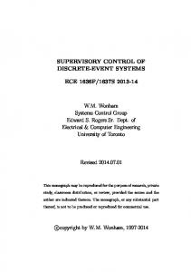
Max-min control systems have been used in [9,5] to model the dynamics of the start-up and completion times of machines connected in serial and/or parallel production lines. Figure 1 shows a serial production line of two machines and one buffer. Assume that the service/process times of the two machines are

u(k) −→

Machine M1 proc.time=m1

f1 (k) −→

Buffer capacity=b

x1 (k) −→

Machine M2 proc.time=m2

x2 (k) = y(k) −→

Fig. 1. A serial (assembly) production line.

constants m1 , m2 , the capacity of the buffer is an integer b ≥ 1, and the transition times to transport machined parts from machine to buffer or from buffer to machine are zero. Let us define by u(k) the arrival time of the materials needed for the kth performance cycle of machine M1 , by y(k) the exit (output) time of the kth product from machine M2 , by si (k) the start-up time of the ith machine, by fi (k) the completion time of the ith machine, and by xi (k) the output time from the ith machine for its kth performance cycle. Note that fi (k) = si (k) + mi , i = 1, 2. The first cycle starts at k = 0 and assume that u(k) = y(k) = si (k) = fi (k) = xi (k) = −∞ for all k < 0 and the buffer was initially empty. If the buffer has infinite capacity (b = ∞), then there is no blocking and x1 (k) = f1 (k) ∀k. But if b < ∞, there is blocking and x1 (k) ̸= f1 (k); i.e., b < ∞ =⇒ x1 (k) = max[f1 (k), x2 (k − b)]

(5)

Thus, M1 cannot output its machined part at cycle k before M2 has finished its task at cycle k − b. But the output time of M2 is identical with its completion time. Combining all the above leads to the following state equations for the output times of the two machines in Fig. 1 (valid for two extreme values of b: b = 1 or b = ∞): [ ] [ ] [ ] ([ ] ) x1 (k + 1) m1 θ x1 (k) m1 + = ∨ + u(k + 1) x2 (k + 1) m1 + m2 m2 x2 (k) m1 + m2 [ ] x1 (k) y(k) = [−∞, 0] + (6) x2 (k) where θ = 0 if b = 1 and θ = −∞ if b = ∞. 2.2

State-Space Models of Nonlinear Filters

A very large class of discrete linear time-invariant systems used in control and signal processing [2,8,13] can be described via the following class of linear


220

difference equations y(k) =

n ∑

ai y(k − i) +

i=1

p ∑

bj u(k − j)

(7)

j=0

Replacing sum with maximum and multiplication with addition gives us the following nonlinear max-sum difference equation [12]  (n )  p ∨ ∨ y(k) = ai + y(k − i) ∨  bj + u(k − j) (8) i=1

j=0

capable of modeling a large class of morphological systems used in nonlinear signal processing and image analysis [10,11,15]. The nonlinear state equations of (1) (or of (3)) can also model the dynamics of nonlinear discrete-time filters of the morphological type described by the above max-sum (or min-sum) difference equation. Specifically, if p = 0, setting x1 (k) = y(k − n), x2 (k) = y(k − n + 1), ..., xn (k) = y(k − 1) and choosing matrices     −∞ 0 −∞ . . . −∞ −∞  −∞ −∞ 0 . . . −∞   −∞       ..  . . T  .. ..  , B =  A= .  . . .  , C = [an . . . a1 ] , D = b0     −∞  −∞ −∞ −∞ . . . 0  b0 an an−1 an−2 . . . a1 models (8) as a special case of (1).

3

Representation of Matrix and Signal Operations by Lattice Dilations and Erosions

Our set of scalars will be R. The triple (R, ∨, ∧) is a complete distributive lattice with partial order the standard relation ≤ among extended real numbers. 3.1

Vector Lattice n

Consider now the vector space L = R , equipped with the following ‘supremum’ and ‘infimum’ operation. Given two vectors x, y ∈ L, their supremum is defined as the vector z = x ∨ y with2 zi = xi ∨ yi , i = 1, ..., n. Similarly we define the ‘infimum’ of vectors by replacing ∨ with ∧. Then, (L, ∨, ∧) is also a complete distributive lattice with an induced partial order 2

Notation: If M = [mij ] is a matrix, its (i, j)th element is also denoted as {M }ij = mij . Similarly, if x is a vector, its ith element is denoted as {x}i or simply xi .


221

defined componentwise; i.e., x ≤ y means xi ≤ yi ∀i. Of interest are operators ψ on L (i.e., vector transformations) that are increasing, i.e., x ≤ y implies ψ(x) ≤ ψ(y). Elementary increasing operators are the translations τv (x) = v + x, which add a scalar v to a vector x componentwise. Actually, the set T = {τv : v ∈ R} of translations forms a commutative group under composition τ v τ r (x) = τ v (τ r (x)) = τ v+r (x). If we define the elementary vectors ei ≡ [−∞, ..., −∞, 0, −∞, ..., −∞]T with a zero at the ith position and −∞ elsewhere, then each vector x = [x1 , ..., xn ]T can be represented as a max of translated elementary vectors: x=

n ∨

xi + ei =

i=1

n ∨

τ xi (ei )

(9)

i=1

Two very important types of increasing operators are the dilations δ and the erosions ε which are defined [16,6] as operators that distribute over sup and inf, respectively: ∨ ∨ ∧ ∧ δ ( xi ) = δ (xi ), ε( xi ) = ε(xi ) (10) i

i

i

i

Two special examples of dilation (δ M ) and erosion (εM ) are, respectively, the max-sum and min-sum ‘product’ of a matrix M with an input vector:

δ M (x) ≡ M + x, εM (x) ≡ M + ′ x

(11)

An operator ψ on L is called translation-invariant or simply a T-operator iff it commutes with any translation, i.e., iff τ ψ = ψ τ ∀τ ∈ T. The following theorem establishes a two-way correspondence between the max-sum and min-sum matrix-based vector transformations and the T-dilations and Terosions. n

Theorem 1. (a) Any translation-invariant dilation δ on L = R can be represented as a matrix-based dilation δ M where M = [mij ] with mij = {δ (ej )}i , and vice-versa. (b) Any translation-invariant erosion ε on L can be represented as a matrixbased erosion εM where M = [mij ] with mij = {ε(ej )}i , and vice-versa. T Proof: ∨n(a) Let δ be a T-dilation on L. For any x = [x1 , ..., xn ] ∈ L we have x = j=1 τ xj (ej ). Hence,   n n n n ∨ ∨ ∨ ∨ δ (x) = δ  τ xj (ej ) = δ (τ xj (ej )) = τ xj (δ (ej )) = δ (ej ) + xj j=1

j=1

j=1

j=1

Hence, by defining the matrix M = [mij ] = [δ (e1 ), ..., δ (en )] with mij = {δ (ej )}i , we obtain n ∨ {δ (x)}i = mij + xj j=1


222

which implies that δ (x) = M + x. Conversely: Consider an operator δ on L defined by δ (x) = M + x. Then, if xk = [xk1 , ..., xkn ]T is an indexed set of vectors, for each i = 1, ..., n we have n n ∨ ∨ ∨ ∨∨ ∨ {δ ( xk )}i = mij + ( xki ) = mij + xki = { δ (xk )}i k

j=1

k

k j=1

k

∨ ∨ Thus, δ ( k xk ) = k δ (xk ) and hence δ is a dilation. Further, for each translation τ v we have for each i = 1, ..., n:   n n ∨ ∨ {τ v (δ (x))}i =  mij + xj  + v = mij + xj + v = {δ (τ v (x))}i j=1

j=1

Thus, τ v (δ (x)) = δ (τ v (x)) and hence δ is also translation-invariant. (b) The proof is identical to that of (a) by replacing dilation with erosion and ∨ with ∧. Q.E.D. 3.2

Signal Lattice

Consider the set Fun(Z, R) of all discrete-time signals f : Z → R with values form R. Equipped with pointwise sup ∨ and inf ∧, this becomes a complete distributive lattice L with partial order the pointwise signal relation ≤. The signal translations are the operators τ i,v (f )(k) = v + f (k − i), where (i, v) ∈ Z × R and f (k) is an arbitrary input signal. An operator on L is called translation-invariant iff it commutes with any such translation. Consider now two elementary signals, called upper impulse (q∨ ) and lower impulse (q∧ ): { { 0, k=0 0, k=0 q∨ (k) ≡ , q∧ (k) ≡ −∞, k ̸= 0 +∞, k ̸= 0 then every signal f can be represented [12] as a sup of translated upper impulses or as inf of translated lower impulses: ∨ ∧ f (k) = f (i) + q∨ (k − i) = f (i) +′ q∧ (k − i) i

i

Consider now operators on L that are dilations (resp. erosions), i.e., systems that distribute over any sup (resp. inf) of input signals. Special cases of dilation and erosion systems are, respectively, the supremal convolution ⊕ and the infimal convolution ⊕′ of two signals f and g defined by ∨ ∧ (f ⊕g)(k) ≡ f (i) + g(k − i), (f ⊕′ g)(k) ≡ f (i) +′ g(k − i) i

i

These two nonlinear convolutions are known in optimization [1], convex analysis [14], and especially in morphological signal processing where they (under


223

the names of signal dilation and erosion) have found numerous applications in nonlinear filtering and computer vision [15,10,11]. The following theorem from [12] characterizes all translation-invariant dilation or erosion systems as nonlinear convolutions of the morphological type between the input signal and the system’s impulse response. Theorem 2. [12] (a) An operator ∆ on the signal lattice Fun(Z, R) is a translation-invariant dilation system iff it can be represented as the supremal convolution of the input signal with the system’s upper impulse response h∨ = ∆(q∨ ). (b) An operator E on the signal lattice Fun(Z, R) is a translation-invariant erosion system iff it can be represented as the infimal convolution of the input signal with the system’s lower impulse response h∧ = E(q∧ ).

4

State and Output Responses

Based on the above lattice representations of max-sum matrix operations, the basic state-space model of a max-sum control system can now be represented via matrix-based dilations: x(k + 1) = δ A [x(k)] ∨ δ B [u(k)] y(k) = δ C [x(k)] ∨ δ D [u(k)]

(12)

Solving the state-space equations by using induction on k yields the state response: (∨ ) k−1 (k) (k−1−i) + B + u(i) x(k) = A + x(0) ∨ A i=0 (∨ ) (13) k−1 k−1−i k = δ A [x(0)] ∨ δA δ B [u(i)] i=0

where A(k) denotes the k-fold max-sum matrix product of A with itself for k ≥ 1 and A(0) = I n where I n is the n × n identity matrix I in max algebra consisting of zeros on its diagonal and −∞ elsewhere. The above result yields in turn the output response: (∨ ) k−1 k k−1−i y(k) = δ C δ A [x(0)] ∨ δC δA δ B [u(i)] ∨ δ D [u(k)] (14) i=0 {z } | {z } | ‘zero’-input resp. y zs (k) ≡ ‘zero’-state resp. Thus, the output response is found to consist of two parts: (i) the ‘zero’-input response which is due only to the initial conditions x(0) and assumes an input equal to −∞, and (ii) the ‘zero’-state response which is due only to the input x(0) and assumes initial conditions equal to −∞. For single-input single-output systems the mapping u(k) 7→ yzs (k) can be viewed as translation-invariant dilation system ∆. Hence, the ‘zero’-state


224

response can be found as the supremal convolution of the input with the impulse response h = ∆(q∨ ) of ∆: ∨ yzs (k) = ∆(u)(k) = u(i) + h(k − i) (15) i

Assuming the system is initially at rest, its impulse response is found to be  k 0 The last two results can be easily extended to multi-input multi-output systems.

5

Elements from Max Algebra

In this section we summarize some results of minimax algebra, mainly from [4], which are useful for our subsequent analysis. m×n

Solving Max-Sum Equations: Let A ∈ R of solutions of A+x=b

m

and b ∈ R . The set (17)

over R is either empty or forms a commutative semigroup under vector ∨. In [4] necessary and sufficient conditions are given for the existence and uniqueness of such solutions. One such result important for our analysis is given next, by using the conjugate matrix A∗ where {A∗ }ij = −{A}ji for all i, j. Theorem 3. [4] Equation (17) has at least one solution iff x = A∗ + ′ b is a solution; and x = A∗ + ′ b is then the greatest solution. Vector Independence: Eq. (17) can also be written as n ∨

a(j) + xj = b

(18)

j=1 m

where a(j) ∈ R , j = 1, ..., n, are the n consecutive columns of A. If xj > −∞ ∀j, we say that b is max-sum dependent on all the a(j), ..., a(n). By negation of max-sum dependence, the vectors a(j), ..., a(n) are called maxsum independent iff none of them is max-sum dependent on the others. A more useful (for our analysis) type of independence is the following. The vectors a(j), ..., a(n) are called strongly max-sum independent (SMI) iff there m exists a finite b ∈ R that has a unique expression of the form (18) with all xj finite and the max of each row and column of A is a finite real. Theorem 4. [4] The vectors a(j), ..., a(n) are SMI iff there exists a finite m b ∈ R such that (17) is uniquely soluble.


225

Matrix Rank: If we can find r columns of A (1 ≤ r ≤ n), but no more, that are SMI, then A is said to have column-rank equal to r. n×n

Graph of a Matrix: Each square matrix A = [aij ] ∈ R can be represented by a directed weighted graph Gr(A) that has n nodes, is strongly complete, i.e., for each pair of nodes there is a corresponding directed graph branch (arc) joining them, and the weight of each arc joining a pair of nodes (i, j) is equal to aij . Consider a path on the graph, i.e., a sequence of nodes P = (i0 , i1 , ..., it ); its length L(P ) and weight W (P ) are defined, respectively, by: L(P ) ≡ # arcs on P = t, W (P ) ≡ ai0 i1 + ... + ait−1 it A path is called a circuit if i0 = it ; the circuit is elementary if the nodes i0 , ..., it−1 are pairwise distinct. For any circuit P we can define its average weight by W (P )/L(P ). Let λ(A) ≡

∨ all circuits P of A

W (P ) L(P )

(19)

be the maximum average circuit weight in Gr(A). Since Gr(A) has n nodes, only elementary circuits (with lenth ≤ n) need be considered in (19). There is also at least one circuit whose average weight coincides with the maximum value (19); such a circuit is called critical. Definite and Metric Matrices: A matrix A is called definite if every circuit in its graph has weight ≤ 0 and at least one such circuit has weight = 0. The metric matrix generated by a matrix A is defined by Γ (A) ≡ A ∨ A(2) ∨ ... ∨ A(n)

(20) n×n

Eigenvalues, Eigenvectors: Given a square matrix A = [aij ] ∈ R , n we say that x ∈ R is an eigenvector of A and λ ∈ R a corresponding eigenvalue of A if A + x=λ+x (21) If we can find finite λ and x satisfying (21), then we say that the eigenproblem is finitely soluble for A. If A is definite, its associated graph Gr(A) contains at least one circuit with zero weight. An eigennode is any node on such a circuit. Theorem 5. [4] Let A be definite. Then: (a) j is an eigennode of Gr(A) iff {Γ (A)}jj = 0. (b) If j is an eigennode of Gr(A), then the jth column of Γ (A) is an eigenvector of A whose corresponding eigenvalue is zero. Thus, columns of Γ (A) that correspond to eigennodes provide eigenvectors for A, which are called fundamental eigenvectors. Two such eigenvectors are called equivalent if their corresponding eigennodes belong to the same critical


226

circuit. Max-sum combinations of non-equivalent fundamental eigenvectors generate the eigenspace of A, whose elements are eigenvectors of A with corresponding eigenvalue = 0. Theorem 6. [4] (a) If the eigenproblem for A is finitely soluble, then every finite eigenvector has the same unique finite eigenvalue, called the principal eigenvalue, which is equal to the maximum average circuit weight of A defined in (19). All finite eigenvectors of A lie in the eigenspace of the definite matrix A − λ(A). The non-equivalent fundamental eigenvectors which generate this space are SMI. (b) The eigenproblem for A is finitely soluble iff λ(A) is finite and Φ(A − λ(A)) has rows and columns whose maxima are finite, where Φ(A − λ(A)) is any matrix whose columns form a maximal set of non-equivalent fundamental eigenvectors for the definite matrix A − λ(A). (c) If A is finite, then the eigenproblem for A is finitely soluble. Periodicity: A definite matrix A has zero principal eigenvalue. Such a matrix is called order-d-periodical if there is an integer k0 such that A(k+d) = A(k) ∀k ≥ k0 . Theorem 7. [3] If A has zero principal eigenvalue and the corresponding critical circuit is unique and has length d, then A is order-d-periodical.

6

Causality, Stability

A max control system initially at rest can be viewed as a translation-invariant dilation system ∆ mapping the input u to the output y. (Assume for brievity single-input single-output systems.) Let h = ∆(q∨ ) be the impulse response of ∆. A useful bound for signals f (k) processed by such systems is their max absolute value over their support: Bf ≡ sup{|f (k)| : f (k) > −∞} Such systems are called bounded-input bounded-output (BIBO) stable iff a bounded input yields a bounded output, i.e., if Bu < +∞ =⇒ By < +∞. The following theorem provides us with simple algebraic criteria for checking the causality and stability of max control systems based on their impulse response. Theorem 8. [12] Consider a max-sum control system ∆ initially at rest and let h = ∆(q∨ ) be its impulse response. (a) The system is causal iff h(k) = −∞ for all k < 0. (b) The system is BIBO stable iff Bh < +∞. In standard linear control the stability of the linear system can also be expressed via the eigenvalues of the matrix A. We have derived a conceptually similar result (stated next) that links the stability of a max-sum control system with the principal eigenvalue of A. (For simplicity, the theorem assumes a unique critical circuit, but it can extended to more general cases.)


227

Theorem 9. Consider a max-sum control system whose matrices A, B, C, D do not contain any +∞ elements. Assume that there is a unique critical circuit of length d corresponding to the finite principal eigenvalue λ(A) of A. Then: (a) If λ(A) = 0, the impulse response of the system is periodic with period equal to d. (b) The system is BIBO stable iff λ(A) = 0. Proof: (a) The zero principal eigenvalue makes the matrix A order-d-periodical. Hence, by (16), there exists k0 such that h(k + d) = h(k) for all k ≥ k0 . (b) If λ is the principal eigenvalue of A, then (a) implies that A(k+d) = dλ + A(k) for all k ≥ k0 . Hence, h(k + d) = dλ + h(k), ∀k ≥ k0

(22)

Further, the absence of +∞ values in the system’s matrices guarantees that h(k) does not have any such values. Now, if λ = 0, then h(k + d) = h(k) ∀k ≥ k0 and hence Bh < +∞. In contrast, if λ ̸= 0, then (22) will drive asymptotically (as k → ∞) the values of |h(k)| unbounded, and hence Bh = +∞. Q.E.D. Example 1 (DEDS): The DEDS with state-space equations (6) has principal eigenvalue λ(A) = max(m1 , m2 ) which is positive since m1 , m2 > 0. Thus, this system is BIBO unstable. Of course, if the impulse response of the system (as is the case with this example) becomes unbounded only asympotically, then our definition of BIBO stability only affects the system if we let it run for an infinite time. In contrast, if we run the system only for a finite time, then its impulse response and output signal remain finite. Example 2 (Recursive Nonlinear Filter): The max control system corresponding to the recursive filter described by (8) has a principal ∨nonlinear n eigenvalue equal to λ(A) = k=1 ak /k. Hence, for this system to be stable, all the coefficients ak must be nonpositive and at least one of them must be zero.

7

Controllability, Observability

A max-sum control system is controllable if the following system of nonlinear equations can be solved and provide the vector u = [u(0), u(1), ..., u(n − 1)]T of input values required to drive the system from the initial state x(0) to any desired state x(n) in n steps:    u(0)    .. x(n) = A(n) x(0) ∨ [A(n−1) + B, · · · , B] +  (23)  . {z } | u(n − 1) C


228

Assuming that the input is dominating the initial conditions, i.e., the second term is greater than the first term of the right hand side, we can rewrite the above as C +u=x (24) where x = x(n) is the desired state. This is a system of max-sum equations which may be solved using the methods of minimax algebra. A necessary condition to find a unique solution of (24), i.e., a unique input vector to drive the system to the state x in n steps is the rank of C to be equal to n, i.e., the columns of C must be SMI. However, in certain applications Eq. (24) may be too strong of a condition and it may be sufficient to solve an approximate controllability problem that has some optimality aspects. Specifically, consider the problem of finding an optimal input vector u as solution to the following optimization problem: Minimize ||x − C + u|| subject to C + u ≤ x

(25)

where the norm || · || is either the ℓ∞ or the ℓ1 norm. Namely, we wish to minimize a norm of the earliness subject to zero lateness. It follows [4] that the solution to the above optimization problem is u = C∗ + ′x

(26)

We note that the optimal controllability solution (26) is actually a lattice erosion, and its optimality can be proven simply by using properties of lattice dilations and erosions. Specifically, to the dilation δ (y) = C + y there corresponds a unique erosion ε(y) = C ∗ + ′ y such that the operator pair (ε, δ ) forms a lattice adjunction [6]. One property of such adjunctions is that the composition δε, known as the opening operator, is antiextensive. Thus, δ (ε(x)) ≤ x and u = ε(x) is the largest solution with δ (u) ≤ x. The above ideas on the controllability problem can also be applied to the observability problem. A max-sum control system is observable if we can estimate the initial state by observing a sequence of output values. This can be done if the following system of nonlinear equations can be solved:       C y(0) u(0)     +   .. .. .. x(0) ∨ [h(n−1), · · · , h(0)] +   =   . . . y(n − 1)

|

C + A(n−1) {z } O

u(n − 1)

(27) Assuming that the first term of the right hand side containing the initial state dominates the second term that contains the input, we can rewrite the above as (28) O + x(0) = y = [y(0), ..., y(n − 1)]T


229

This max-sum matrix equation can be solved either exactly or approximately by using the same methods as for the controllability equation. The general solution is then ˆ (0) = O∗ + ′ y x (29) + ˆ (0) ≤ y. and has the property that it is the largest solution with O x

8

Feedback

Consider a max control system described by the state space equations (12) and let its input signal u(k) be the max of a feedback of the state and a reference signal w(k). The state feedback law considered is u(k) = w(k) ∨ (F + x(k))

(30)

where F is the feedback matrix. Then the new state space equations will be x(k + 1) = [A ∨ (B + F )] + x(k) ∨ B + w(k) y(k) = [C ∨ (D + F )] + x(k) ∨ D + w(k)

(31)

Thus, the use of feedback can affect the principal eigenvalue of the system, as well as its controllability and observability. We illustrate a possible effect of feedback on the system’s eigenvalue via the example of the DEDS of Fig. 1. Suppose as in [9] that, we want to design this system to have cyclic behavior, i.e., x(k + 1) = λ + x(k)

(32)

where λ is a constant positive number (the cycle time). The original statespace equations (6) are x(k + 1) = [A + x(k)] ∨ [B + u(k + 1)]

(33)

If we use a state feedback of the form u(k + 1) = F + x(k) , F = [r1 , r2 ]

(34)

then from (33) and (34) we obtain λ + x(k) = [A ∨ (B + F )] + x(k)

(35)

Thus the problem reduces to finding the principal eigenvalue of [ ] [ ] m1 θ m1 + r 1 m1 + r 2 Q = A∨(B + F ) = ∨ (36) m1 + m2 m2 m1 + m2 + r1 m1 + m2 + r2 and the corresponding eigenvector x(0). Setting r1 = r2 = 0 yields the following matrix Q and its eigenvalue and eigenvector: [ ] [ ] m1 m1 m1 Q= =⇒ λ(Q) = m1 + m2 , x(0) = (37) m1 + m2 m1 + m2 m1 + m2 Since x1 (0) = m1 + u(0) and x2 (0) = m1 + m2 + u(0), it follows that the choice of feedback F = [0, 0] and initial input u(0) = 0 achieves the above cyclic behavior with cycle time λ = m1 + m2 .


230

References 1. R. Bellman and W. Karush, “On the Maximum Transform”, J. Math. Anal. Appl., 6, pp. 67–74, 1963. 2. W. L. Brogan, Modern Control Theory, Quantum Publ., New York, 1974. 3. G. Cohen, D. Dubois, J.P. Quadrat and M. Viot, “A Linear System Theoretic View of Discrete Event Processes and Its Use for Performance Evaluation in Manufacturing”, IEEE Trans. Autom. Control, vol. 30, pp. 210-220, 1985. 4. R. Cuninghame-Green, Minimax Algebra, Springer-Verlag, New York, 1979. 5. A. Doustmohammadi, “Modeling of Discrete Event Dynamic Systems based on Petri Nets and Minimax Algebra Approach”, PhD thesis proposal, Georgia Inst. Tech., Atlanta, 1993. 6. H.J.A.M. Heijmans, Morphological Image Operators, Acad. Press, Boston, 1994. 7. Y.-C. Ho, Ed., “Special Issue on Dynamics of Discrete Event Systems”, Proc. IEEE, vol. 77, Jan. 1989. 8. T. Kailath, Linear Systems, Prentice-Hall, N.J., 1980. 9. E. W. Kamen, “An Equation-Based Approach to the Control of Discrete Even Systems with Applications to Manufacturing”, Proc. Int’l Conf. on Control Theory & its Applications, Jerusalem, Israel, Oct. 1993. 10. P. Maragos and R. W. Schafer, “Morphological Filters - Parts I & II”, IEEE Trans. Acoust., Speech, Signal Processing, vol. 35, pp. 1153-1184, Aug. 1987. ibid, 37:597, Apr. 1989. 11. P. Maragos and R. W. Schafer, “Morphological Systems for Multidimensional Signal Processing”, Proc. IEEE, vol. 78, pp. 690-710, Apr. 1990. 12. P. Maragos, “Morphological Systems: Slope Transforms and Max–Min Difference and Differential Equations”, Signal Processing, vol. 38, pp. 57-77, 1994. 13. A. V. Oppenheim and R. W. Schafer, Discrete-time Signal Processing, PrenticeHall, N.J., 1988. 14. R. T. Rockafellar, Convex Analysis, Princeton Univ. Press, Princeton, 1972. 15. J. Serra, Image Analysis and Mathematical Morphology, NY: Acad. Press, 1982. 16. J. Serra, Ed., Image Analysis and Mathematical Morphology, Vol.2: Theoretical Advances, NY: Acad. Press, 1988.


Min-Max Control with Application to Discrete Event ... - CVSP - NTUA

Min-Max Control with Application to Discrete Event ... - CVSP - NTUA

Suggest Documents

Slope transforms - CVSP - NTUA

Differential Morphology - CVSP - NTUA

Slope transforms - CVSP - NTUA

Speech Event Detection using Multiband Modulation ... - CVSP - NTUA

discrete event simulation with application to computer

Tamil liquids and stops - CVSP - NTUA

Audio-Assisted Movie Dialogue Detection - CVSP - NTUA

Tamil liquids and stops - CVSP - NTUA

MOVIE SUMMARIZATION BASED ON AUDIOVISUAL ... - CVSP - NTUA

Control of Discrete-Event Systems with Partial

Discrete Event Simulation with Application to Computer - Springer Link

Discrete Event Simulation with Application to Computer - Springer Link

SUPERVISORY CONTROL OF DISCRETE-EVENT

Image Decomposition into Structure and Texture ... - CVSP - NTUA

Harmonic analysis and restoration of separation ... - CVSP - NTUA

Bayesian Inference on Multiscale Models for Poisson ... - CVSP - NTUA

Multi-room speech activity detection using a ... - CVSP - NTUA

Speech Analysis and Feature Extraction using Chaotic ... - CVSP - NTUA

Leveling cartoons, texture energy markers, and image ... - CVSP - NTUA

Adaptive and Constrained Algorithms for Inverse ... - CVSP - NTUA

Lattice Image Processing: A Unification of ... - CVSP - NTUA

spatial bayesian surprise for image saliency and ... - CVSP - NTUA

Robust Energy Demodulation Based on Continuous ... - CVSP - NTUA

analysis of kirlian images: feature extraction and ... - CVSP - NTUA