Minerva: Distributed Tracing and Debugging in Wireless Sensor Networks Philipp Sommer
Branislav Kusy
Autonomous Systems Lab, CSIRO Brisbane, QLD, Australia
Autonomous Systems Lab, CSIRO Brisbane, QLD, Australia
[email protected]
ABSTRACT Development of wireless sensor network applications remains a challenge, due to lack of visibility into the global network state. Debugging instrumentation using printf-like instructions affects the execution timing and non-intrusive approaches, such as JTAG, have not been used beyond a single node due to their high cost. This paper presents Minerva, a testbed architecture for distributed debugging of wireless sensor networks. At the core of our architecture is a flexible debug board installed at each node. The board design is driven by cost-efficiency of the testbed instrumentation and provides access to the onchip debug port of the sensor node’s processor. We focus on three main debugging modalities: (i) non-intrusive networkwide tracing of the internal state of individual nodes; (ii) synchronous stopping of the whole network on a breakpoint; and (iii) distributed assertion checking. We demonstrate the debugging capabilities of Minerva in use-cases based on well-known sensor network protocols in a 20-nodes indoor testbed. Our results indicate that Minerva provides non-intrusive, network-wide debugging of sensor network applications at a low cost.
Categories and Subject Descriptors D2.5 [Software Engineering]: Testing and Debugging
General Terms Algorithms, Design, Experimentation
Keywords Wireless Sensor Network, Tracing, Debugging, JTAG
1. INTRODUCTION Wireless sensor networks (WSNs) have become an invaluable tool for the observation of physical phenomena at large scale and with high fidelity. To allow for high data yield
Copyright is held by the owner/author(s). Publication rights licensed to ACM. SenSys’13, November 11–15, 2013, Rome, Italy. Copyright 2013 ACM 978-1-4503-2027-6/13/11 ...$15.00.
[email protected]
and continuous operation when deployed in challenging environments, hardware and software components need to be highly reliable and well tested. Debugging wireless sensor networks is known to be a notoriously hard task. Therefore, a typical development cycle of a sensor network application encompasses several iterations of simulations and experiments on the target hardware. Simulations provide a simple and scalable way to gain a rough approximation of the expected execution performance, but are often not capable of fully capturing the low-level behavior of the hardware platform. To bridge this gap, a number of wireless sensor network testbeds were built in the last decade that allow researchers to assess the performance of applications or sensor network protocols under realistic conditions [2, 3, 7, 15, 29]. Sensor network testbeds facilitate an easy access to sensor nodes through remote programming and monitoring of node output. However, testbeds provide only limited visibility in the state of individual sensor nodes, using techniques such as writing to the serial port or toggling output pins. Determining the state of a distributed application running across a number of sensor nodes or the state of an underlying network protocol is a challenge since it requires instantaneous knowledge about all nodes in the network. Most microcontrollers used in common sensor node platforms provide an integrated debugging module that can be accessed by the JTAG interface. Although initially designed for electrical testing of boards, JTAG evolved into a common debugging tool used for setting breakpoints, halting the microcontroller, or stepping through the program code. Due to the high cost of JTAG adapter hardware and often proprietary software necessary for JTAG-enabled debuggers, sensor network testbeds have not harnessed the powerful capabilities of debug modules at the network scale so far. In this paper, we introduce Minerva, a distributed tracing and debugging tool for wireless sensor networks. The key idea is to access the debugging port of sensor nodes from an observer node co-located with each sensor node in a testbed. Using the integrated debug hardware has several benefits over traditional software-based debug approaches. First, the debug port provides non-intrusive debugging that is independent of the operating system running on the sensor node. By accessing the debug port from an external device, the processor of the sensor node can be halted and resumed. Importance of non-intrusive access to source code execution was demonstrated by the Aveksha platform [27]. Aveksha provides tracing of events and breakpoints for a single node by co-locating a debug board with the sensor node under test and stores the trace data locally. Minerva extends this ap-
proach by connecting the debug board to a testbed observer, which is part of an out-of-band backbone network, e.g., Ethernet. By accessing the debug board from the observer, it becomes feasible to stop all nodes within the sensor network simultaneously. Additionally, read and write access to the internal memory bus of the processor allows for a detailed insight into the state of sensor nodes while they are running. By combining the trace information from individual nodes at a central instance, we get visibility into a network-wide state of sensor network applications. Minerva further expands this functionality by providing real-time assertions on the global state of applications or network protocols. When a global assertion fails, the network can be halted for closer inspection, or a memory snapshot can be taken for further analysis. This paper makes the following contributions towards debugging of sensor network applications in a testbed setting: • We present the hardware and software architecture of Minerva, a novel testbed architecture which allows network-wide tracing and debugging using the integrated debug port of sensor nodes. • We describe how Minerva can be used for debugging WSN applications at the network scale and study its performance under realistic conditions. • We introduce testbed support for non-intrusive networkwide assertion checking. The rest of this paper is organized as follows: we overview debugging modalities for WSNs in Section 2 and introduce the system architecture of Minerva in Section 3. We follow by an overview of the individual debugging modalities (Section 4) and introduce distributed assertions in Section 5. We present several case studies for debugging network protocols with TinyOS (Section 6). Finally, we outline related work in Section 7 and conclude in Section 8.
2. DEBUGGING METHODS In this section, we provide an overview of debugging methods available on embedded sensor network platforms, followed by a brief overview of the JTAG protocol used for debug access. Figure 1 compares the debugging modalities provided by Minerva and other hardware-based testbed architectures. Flocklab [15] employs a network of observer nodes to provide logging of serial output, and GPIO monitoring and actuation. Aveksha [27] provides access to the node’s debug port using JTAG from a debug board connected to the node. Both Flocklab and Aveksha support power profiling of applications as a complimentary debugging method.
2.1
Serial Output
The approach most commonly used in testbeds is to use the node’s serial communication interface (e.g., UART) for emitting debug packets or printf() output that can be observed and logged by the testbed. While this approach of code instrumentation provides a flexible method for observation of code execution flow, it comes with a significant overhead in terms of the execution time. Since serial ports of microcontrollers integrated on common node platforms operate at relatively slow speeds (e.g. 115 kBaud), the microcontroller spends a significant amount of clock cycles
preparing and transmitting characters for each printf() statement. Consequently, code instrumentation for debugging purposes might significantly change the timing of code execution, which can lead to a modified behavior of the application under test.
2.2
Output Pin Monitoring
An alternative approach uses digital output pins of the microcontroller to indicate certain events by changing the pin state accordingly. Pin monitoring enables fine-grained tracing of code execution and limits the overhead of code instrumentation to a few clock cycles. However, this approach requires special tools, such as an oscilloscope or logic analyzers [15], to trace execution at a fine-grained level. In addition, a single digital output line can only represent binary information, and thus the number of states that can be traced simultaneously with logic analyzers is limited.
2.3
Debug Port (JTAG)
The debug port available in many microcontrollers bridges the gap between external debug device and internal debug logic of the core. Typically, the debug port (slave) is connected via a debug access protocol (e.g., JTAG) to a debugging tool (master). The debugging process is usually controlled by a specialized software tool such as the GNU Debugger (GDB). Depending on the capabilities offered by the platform, several invasive (breakpoints/watchpoints) or non-invasive debugging techniques (memory access) are possible. Furthermore, the debug port may also be used for programming a new binary image to the microcontroller’s flash memory. The debug logic can insert breakpoints at a specific location in the code to halt the processor. Once the processor reaches a breakpoint, code execution stops and the core enters debug mode. While the core is halted, GDB can be used to single-step through the code and inspect registers or memory within the system. Breakpoints are an intrusive way of debugging since the core stops fetching and executing instructions. Consequently, interrupts signaled by peripherals (e.g., timer or radio interrupts) will not be handled, which might lead to undesired behavior. Tracing provides a non-intrusive approach to debugging where certain events or internal state is observed from outside without the need for stopping the processor. Depending on the frequency of events we are interested in, e.g., monitoring the value of the program counter (PC), a large amount of trace data is generated. Triggers can be used to filter for specific events of interest, for example when a certain memory address is read or written with a specific value. However, the bandwidth of the debug port limits the frequency of events that can be observed.
2.3.1 JTAG Protocol JTAG is a widely used IEEE standard for accessing debug ports of microcontrollers. JTAG specifies a four pin interface between the host (master) and the target (slave): test data out (TDO), test data in (TDI), test clock (TCK), test mode select (TMS). A device can expose multiple test access ports (TAP) which are connected in series in a scan chain. The clock line is driven by the host and data is shifted into the target (TDI) and shifted out of the target (TDO) with each clock cycle. The TMS/TCK pins are used to switch between the different states as defined by the JTAG specifi-
Target
Controller
Observer
Minerva
Cortex-M3 Atmega1281 MSP430
Aveksha
Cortex-M3
Flocklab
Backend Network
Debug Board + PandaBoard
SERIAL PORT JTAG
SERIAL PORT
Flocklab Board + Gumstix
POWER GPIO
Observing execution through printf Memory tracing
Server
Assertions + Halt/resume
Observing execution through printf Power tracing
Server
Pin tracing/actuation
POWER
MSP430
JTAG
Telos Debug Board (MSP430 + FPGA)
GPIO
Figure 1: Overview of debugging architectures for wireless sensor networks: Minerva and Flocklab use outof-band observers to monitor and control the nodes. Minerva’s testbed controller collects and processes trace data from observers and is able to synchronously halt/resume the sensor nodes in the testbed. Aveksha provides JTAG access for tracing and breakpoints but only stores data locally, thus has no consistent global view of the network at runtime. cation. Data can be shifted into two registers of the TAP: an instruction register (IR) and a data register (DR). On each clock cycle, a new bit is written into the register through the TDI line, while the existing content is shifted out of the TAP through the TDO line. While the JTAG protocol provides a standardized interface to access a TAP, the size and purpose of the instruction and data registers depend on the specific implementation of the TAP. Depending on the device vendor, the specifications how to access the internals of the debug port might not be publicly available.
3. SYSTEM ARCHITECTURE Minerva is a hardware-software architecture for distributed debugging of wireless embedded systems. It combines target sensor nodes that form the sensor network and a testbed architecture for control and monitoring. Minerva has been designed as a debugging tool for indoor or outdoor testbed deployments, where reliable out-of-band network connectivity (e.g. Ethernet) is available and power for the observer nodes is not constrained. The focus of this work is on the non-intrusive observation of execution of an application running on the sensor network through memory tracing. Therefore, we have not integrated power tracing as a debug method to our hardware architecture as this is complimentary to our approach. At the core of Minerva is an extension board for the sensor node, which provides access to the debug port of the node’s embedded processor. Observer nodes are connected to the extension board and continuously monitor sensor nodes. Observers are also connected with a testbed controller over a backbone out-of-band network. A high-level overview of Minerva’s architecture is shown in Figure 1. In the following, we provide a detailed discussion of the different Minerva components.
3.1
Node Platform
We use the Opal platform in this paper, although the general ideas proposed here apply to any standard microcontroller featuring a debug port accessible via a JTAG-like interface. A node platform needs to provide the following
hardware capabilities in order to be integrated within the Minerva debugging framework: • Debug port interface (JTAG/Serial Wire Debug/SpyBi-Wire) • Register/memory access through debug port • Breakpoints/watchpoints Most modern microcontroller architectures provide hardware debugging ports, e.g., ARM Cortex processors or the Enhanced Emulation Module (EEM) on the MSP430 series.
3.1.1 Opal Platform The sensor node platform that we used is the Opal platform [10]. It features an Atmel SAM3U microcontroller with integrated ARM Cortex-M3 core. The SAM3U4E is a powerful processor running at clock frequencies of up to 96 MHz and providing 256 KBytes of program flash, 50 KBytes of SRAM, and flexible I/O options (ADC, UART, SPI, I2C, and USB). Furthermore, Opal has two IEEE 802.15.4 compatible radio transceivers (Atmel AT86RF212/AT86RF231) for wireless communication in the 900 MHz and 2.4 GHz ISM bands.
3.1.2 Cortex-M3 Debug Interface The ARM Cortex-M3 core is a 32-bit RISC processor implementing the ARMv7-M architecture. The design of the processor core can be licensed from ARM by other manufacturers for integration in custom products. The debug port of the Cortex-M3 provides two different interfaces: JTAG and the Serial Wire interface. Serial Wire is a half-duplex alternative to JTAG which requires only two pins. The ARMv7 debug architecture allows us to determine and modify the state of the processor from the outside. To this end, the debug adapter connects to the JTAG test access port (TAP), which provides register access for reading and writing from/to the internal memory access ports. The Core Debug Access Port, provides a set of registers to control the debug operation of the processor. For example, the debugger can halt, single step or resume the processor by setting the
corresponding command bit in the debug control register. Furthermore, it can query the processor state to determine when the core reached a breakpoint. Another nice feature of the debug interface is the access to the Cortex-M3’s internal system bus that is provided through the Memory Access Port. It allows the debugger to access the internal SRAM and memory-mapped peripherals for read and write operations. Access to memory through the debug port has a lower priority than bus access initiated by the processor itself to avoid conflicts.
3.2
Target Debug Board
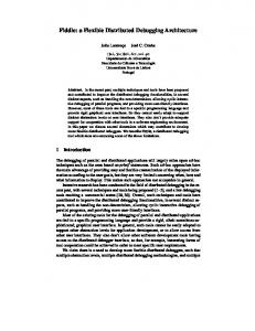
Target debug board is the only custom designed hardware in our testbed. In addition to the access to the debug port, the board also provides USB access to the serial port of sensor nodes. The cost of the board is almost the same as a good quality USB-serial converter that a testbed would have to use anyways. We designed the board to stack on top of the Opal sensor nodes using 2 x 60 pins expansion connectors. FTDI FT2232H. At the core of the debug board is the FTDI FT2232H integrated circuit, as illustrated in Figure 2. It provides two high-speed USB 2.0 endpoints which can be independently configured for different serial or parallel protocols. The chip is widely used as a serial to USB converter on embedded platforms. In our case, Channel B is connected to the debug port of the Cortex-M3 core, while Channel A is connected to the serial port (UART) of the Opal node. We also connected the ERASE and RESET lines of Opal to the FTDI chip to facilitate reprogramming of the processor. One special feature of FT2232H is its support of the MultiProtocol Synchronous Serial Engine (MPSSE). Special control commands sent over the USB endpoint of the device are converted into JTAG sequences on the output lines. The FTDI chip processes incoming command sequences in a FIFO manner and sends the response back to the USB host. While this approach provides great flexibility for different application scenarios, it relies on software on the host for driving the I/O operations. However, we are able to achieve clock frequencies of up to 12 MHz on the JTAG bus. Debug Board
Sensor Node Cortex-M3 (SAM3U)
FTDI FT2232H USB
Channel A: UART
Channel B: JTAG
TX RX TCK TDI TDO TMS
UART Debug Port
Core Peripheral Memory
Figure 2: Minerva debug board: FTDI chip converts JTAG instructions sent by the PandaBoard into physical JTAG signals for SAM3U.
3.3
Target Observer
The observer node communicates between the debug board attached to a sensor node and the testbed controller.
3.3.1 Hardware Architecture We use the PandaBoard embedded platform for our observer nodes, which is a low-cost embedded platform based on the Texas Instruments OMAP 4430 system on a chip. It features four USB ports, Ethernet, HDMI output and Wifi/Bluetooth support. We run Ubuntu with Linux kernel
Figure 3: Testbed observer with Opal node and debug board connected to the PandaBoard. 3.4.11 on the PandaBoards. All observer nodes are connected to our campus network infrastructure using Ethernet and are powered from a wall outlet. Figure 3 depicts the Opal sensor node connected to the observer node.
3.3.2 Software Architecture The software on the observer node is built around the Open On-Chip Debugger (OpenOCD)1 , which is an opensource library for debugging embedded devices that supports JTAG operations using the FT2232H chip on our debug board. OpenOCD complements a debugging toolchain by providing a remote debug target to which GDB can connect. GDB sends control messages to OpenOCD, which then talks to the debug port of the processor and sends the reply back to GDB. Although OpenOCD is specific to the ARM Cortex-M3 architecture, Minerva could use different debugging libraries (e.g., MSPDebug for MSP430 or AVaRICE for Atmel AVR architectures) for other platforms. Remote control interface. We implemented a remote control interface on top of OpenOCD to receive control commands from the testbed controller. The observer listens for UDP multicast packets addressed to a specific port. We opted for UDP multicast due to its efficiency and speedy connection setup. Replies from the observer nodes are sent back to the testbed controller using UDP unicast packets. Request for changes in the state of the observers (e.g., node halted or resumed) are confirmed using an acknowledgment UDP packet. Polling. The observer can be instructed to periodically poll the content of one or multiple addresses in the system memory of the sensor node to detect changes in the internal state of the application running on the node. This approach will be explained in more detail in Section 4. The testbed controller is notified using a UDP unicast packet when a change is detected.
3.4
Testbed Controller
Testbed operation is controlled by the testbed controller. It is responsible for setup, start, monitoring, and teardown of each testbed run. The testbed controller exposes a simple web based interface, implemented in Python, to upload a binary image to the nodes in the network. We use the symbol table of the image to map between global variables and corresponding addresses in the system memory of the sensor node. 1
http://openocd.sourceforge.net
Scripting of tests. In order to offer full flexibility for control and monitoring, we provide users with a Python scripting interface that allows users to reset, halt, and resume the nodes within the testbed and to enable or disable tracing of memory locations. In addition, users specify a callback method that is called whenever the state of the watched memory location changes. This allows users to implement flexible assertions on the state of the network (see Section 5) or log the timeline of events to a database or file for further analysis or visualization.
4. DEBUGGING WITH MINERVA In this section, we describe debugging complex sensor network applications using Minerva. Our approach complements the existing set of testbed debugging modalities (e.g., printf() output, pin monitoring, and power profiling) with: • Tracing: non-intrusive tracing of a node’s internal state; • Control: ability to synchronously halt and resume the whole testbed; • Checkpoints: ability to collect snapshots of selected memory areas of a node; and • Assertions: support for real-time assertions on the global network state. Existing testbeds let the user schedule a test run and offer the results for download afterwards. Since this approach allows to identify the occurrence of problems only after the test has been completed, another series of tests is usually necessary to narrow down the exact cause. Debugging a sensor network with Minerva is radically different from the way existing testbeds work. The realtime monitoring capabilities of Minerva provide a user (or a script) with interactive control of the testbed. Therefore, the cause of potential problems can be assessed immediately after they occurred. Furthermore, our approach is agnostic of the operating system (e.g., Contiki, TinyOS) running on the sensor nodes since debug operations operate at the machine level rather than being implemented in additional software modules or libraries. Therefore, no additional code instrumentation is needed for debugging. In contrast to invasive debugging methods such as printf() or logging to flash storage, Minerva does not introduce delays or alter the timings of code execution on the node, since the node state is only accessed through the debug port of the microcontroller. Thus, our approach avoids Heisenbugs, which are bugs that disappear when modifying the program for debugging [31]. In the following, we describe Minerva’s debugging capabilities in more detail.
4.1
Tracing
The debug port of the Cortex-M3 processor enables to read from the system memory regardless in what state the processor is. Therefore, in contrast to GDB, which only allows to inspect the memory when the processor is at a breakpoint, the observer can periodically poll for changes, even when the processor is currently running. Thus, tracing is the least intrusive debugging method offered by Minerva, since it does not require to stop the processor. The
observer uses address information from the symbol tables of currently executed binary image to poll for memory changes. Tracing is initiated using a subscription mechanism where the testbed controller sends a polling request for a specific memory address and data length to an observer. Until the subscription for this address is revoked by the controller, the observer periodically polls the address for changes. To minimize the amount of network traffic caused by polling, the observer only sends a packet for the start value and a notification whenever the value has changed. The system clocks of all observers and the testbed controller are synchronized using NTP [18]. An update notification to the testbed controller is sent as a UDP packet, which includes the current timestamp, sequence number, memory address, and the corresponding variable value. Memory Access. Read access to the memory for tracing requires the memory access port of the debug port to be configured with the corresponding memory address location. Afterwards, the memory access port reads from the system memory over the internal high-speed bus and writes the result into the data register of the memory access port (see Section 3). Consequently, each memory access requires a certain sequence of JTAG state transitions being initiated by the FTDI chip connected to the JTAG port. Hardware support for tracing. The Cortex-M3 debug architecture offers dedicated hardware support for memory watchpoints and tracing through the integrated Data Watchpoint and Trace Unit (DWT). Data watchpoints in the DWT can be configured using four registers which define address and data masks. The DWT monitors the system bus for memory read and write instructions. Upon match, it sets a flag in the DWT status register and it generates a trigger as configured: a memory watchpoint exception to halt the processor, or it generates a packet on the trace output line. However, the trace output on the SAM3U microcontroller is shared with the TDO pin used by the JTAG protocol. Therefore, the serial trace output is not available while JTAG is active. Concurrency of memory access. Instruction fetches, data, and debug access to the system memory space are performed over the same internal 32-bit bus. However, data access and instruction fetches by the core have higher priority than the debug access. Therefore, debugging will not interfere with regular operation of the core as debug access has to wait until the higher priority operations are completed.
4.1.1 Software Support Memory tracing with Minerva requires information about the address and data type (e.g., uint8 t, int16 t, uint32 t) of global variables. This information can be extracted from the symbol table of the binary image and is independent of the operating system used. nesC annotations. We leverage variable attributes provided by the nesC language [5] as a simple mechanism to annotate variables of interest in the application source code. Global variables of a nesc module which are annotated with the trace attribute will be automatically added to the list of watched memory locations. module MyComponentP { ... } implementation { uint16_t myState @trace(); }
When compiling a nesc/TinyOS application with the debug make option, the nesc compiler will dump a list of variables annotated with the trace attribute to a XML file in the build directory. This file will be read by the tracing application running on the testbed controller to setup variables to watch for changes. The exact memory location and size of the corresponding variables can be determined by inspecting the symbol table in the binary image. Python interface. Alternatively, Minerva’s Python interface allows to setup watched variables if more flexibility is required, e.g., when the set of watched variables needs to be changed dynamically.
printf()
from minerva import model, monitor
Printf output. As we discussed before, code instrumentation using printf() statements has a significant overhead for processing and communication. Figure 6 shows a timeline of events during a single printf() command that is outputting 4 bytes. Invocation of the printf() method triggers the underlying C library to process the input parameters and store the corresponding output string in memory. Next, characters will be written to the serial line one by one. The UART peripheral module of the MCU generates an interrupt after each character transfer has been completed. This will wake up the MCU and it will write the next character in the buffer to the UART.
UART
# load symbol from binary symbols = model.load_symbols(binary) myState = symbols["MyComponentP$myState"]
MCU
# add watchpoint monitor.add_watchpoint(myState)
0.0
0.1
0.3
0.2
0.4
0.5
Time [ms]
4.1.2 Benchmark Results
Figure 6: Overhead of printf() output on Opal.
TCK
We compare the performance of memory tracing with other code instrumentation methods, namely printf() and GPIO instrumentation. JTAG performance. Figure 4 shows a sequence of bus transfers on the JTAG interface during memory tracing. We initiate JTAG access from PandaBoard as fast as possible. A single JTAG access to read 4 bytes from the system memory takes roughly 26 µs. However, access to the system memory is initiated by the debug port hardware component and not through software instructions executed by the processor. Therefore, the timings of the application code are not changed by the JTAG access. It takes the monitoring application on the PandaBoard around 500 µs to setup a read access, transfer the command to the FTDI using USB, and process the result. We measured the time interval between consecutive read operations on the JTAG interface using a logic analyzer for 26,000 samples. On average, a read access is initiated every 610.14 µs with a standard deviation of 78.37 µs. Depending on the scheduling of the monitoring process by the Linux scheduler, the interval may vary, as shown in Figure 5.
0
1
3
2
5
4
6
7
Time [ms]
Figure 4: Timeline of JTAG access to the CortexM3 debug port for memory tracing.
GPIO instrumentation. The output level of general purpose digital input/output (GPIO) pins of the MCU can be changed with only a few processor instructions. In fact, the SAM3U microcontroller requires 2 instructions with a total of 5 clock cycles to set a GPIO pin. Therefore, it allows code instrumentation with minimal overhead in terms of execution time and at a high frequency of events of interest. However, it only allows to differentiate between two different states, or otherwise, the state of the pin might become ambiguous. Comparison and limitations. We summarize our findings in Table 1. Minerva provides high expressiveness without incurring any overhead on the microcontroller as no additional code needs to be executed. The latency of memory tracing determines the maximal frequency of changes to the monitored variables that can still be detected. For example, pin tracing is better suited to detect changes which occur at a very high rate, for example, when instrumenting a local variable within a for loop of a device driver. However, we argue that in the case of testbed experiments the focus is on capturing the node state at a higher level of abstraction, such as at the network protocol or application layers. Examples of such variables of interest include routing tables (e.g., parent node in CTP) or hop counts for network flooding. Therefore, the maximum number of incoming packets within a time interval gives an upper bound on the rate at which such variables can change.
0.025 0.020
Minerva GPIO printf
0.015 0.010 0.005 0.000
0
200
400
600
800
1000
Overhead (µs per bit) 0.05 182
Latency (ms) 0.61 0.001 1.0
Expressive Capability High (Data) Low (Bits) Extended High (Data+Comments)
1200
JTAG Tracing Interval [us]
Figure 5: Distribution of the interval between subsequent JTAG access operations to the Cortex-M3 debug port for memory tracing.
Table 1: Memory tracing performance using different techniques on Opal platform.
4.2
Start/Stop Debugging
Stopping a sensor node by setting the processor into debug mode is an intrusive operation that might have a significant impact on the execution of the application code. For example, halting the processor core will prevent execution of interrupt handlers signaled by internal or external peripherals (e.g., timers, radio transceiver, sensor interrupts). The process of resuming the application after it was stopped at a breakpoint, therefore, is a challenge. Minerva provides techniques and operating system hooks to prevent the system from entering an undefined state, which has not been anticipated when the software logic has been developed.
4.2.1 Debug Mode Description Node-level debug mode. Cortex-M3 processor might enter debug mode for two reasons: (i) when a breakpoint or memory watchpoint is hit during code execution and (ii) when the C_HALT bit in the control register of the debug access port is written. Furthermore, it is also possible that the application running on the node triggers the processor to enter debug mode. The control register of the debug access port is also visible from the system memory space. Therefore, a node can enter the debug mode from the program code. However, the debug module has to be enabled beforehand by writing the C_DEBUGEN bit, which can only be done through the external debug port. Network-wide debug mode. Minerva provides a simple method to synchronously stop a sensor network under test. Using the backbone network, we employ UDP packets sent to an IP multicast address in the same subnet to quickly propagate a stop request from the testbed controller to all observers. IP Multicast enables one-to-many communication without the need to replicate packets for each subscriber. Therefore, the jitter between the time of arrival of a stop request at different observers can be kept as small as possible. Since UDP communication provides no automatic retransmission, we send another UDP packet from the observers to the testbed controller as an acknowledgment when the node has been stopped. Our experiments show almost no lost UDP packets, if a local area network is used to connect observers with the controller. Minerva cannot execute network-wide start/stop debugging in a completely synchronous manner due to the time of arrival jitter of UDP packets. Specifically, Minerva is not suitable to debug events that interact with the application on a microsecond level. However, it is useful for debugging higher level application functionality where millisecond accuracy is sufficient. Even for the higher level application code, Minerva needs to ensure that the whole network stopped in a consistent state and we discuss this in relation to distributed assertions later in Section 5.
4.2.2 Timer Consistency Entering the debug mode immediately stops the processor clock. However, the master clock which is used as a clock source for peripherals of the SAM3U microcontroller is kept running. The SAM3U features a power management controller (PMC), which provides individual control over the clocks of different peripherals such as timers, UART, SPI, and others. Therefore, the observer node can disable selected peripherals when the processors enters debug mode and restore the state of the PMC before the processor is resumed. Since this allows to effectively freeze the hardware
timers of the MCU, the software timer modules in TinyOS or Contiki will resume their operation afterwards without missing timer events.
4.2.3 Application Consistency through OS Hooks Although Minerva is operating system agnostic, adding additional code components might help to avoid potential problems when stopping the application running on every node within the testbed. As a possible future extension, Minerva could politely ask the application to enter a debug mode rather than forcing the processor to enter debug mode immediately and thus potentially compromising the running application. This can be implemented by indicating a pending debug request from the testbed by setting a status flag in the TinyOS or Contiki scheduler. The scheduler will then execute a special method to transfer the system and peripherals into a safe state before entering debug mode, for example by setting the radio or serial port into idle mode.
4.2.4 Benchmark Results We evaluate the latency of synchronously stopping a network from the testbed controller. The experiment setup includes three PandaBoards, one taking the role as the controller and the other two are observers. The controller periodically sets an output pin and sends the stop command to the observers. We record the time interval between the controller sending the command and the exact time when the processor of the sensor node has been stopped by setting an output pin of the Cortex-M3 MCU through the debug port. The measurement results for a total of 52,772 control packets are shown in Figures 7 and 8. The results show that the sensor node has been stopped by the observer roughly 1.55 milliseconds after the command has been transferred by the testbed controller. The jitter between different nodes is smaller than 0.141 ms with a probability of 95%. Comparison with network flooding. Using an efficient network flooding protocol, the node stop command will propagate through the sensor network within a few milliseconds for reasonable network diameters (e.g., flooding using Glossy [4] takes around 2.4 ms on the 8-hop MoteLab testbed). However, the performance of existing approaches employing radio packets forwarded within the sensor network might be affected by interference and the radio dutycycle of intermediate nodes (e.g., when using low-power listening). Minerva is leveraging the out-of band network connection between the controller and observers to send commands to halt/resume sensor nodes, which offers high reliability, low latency and allows to stop the network any time regardless of the low-power state of the node’s radio.
4.3
Memory Checkpoints
Sensornet checkpointing takes a snapshot of the node state ¨ which can then be replayed in a simulation tool. Osterlind et al. [20] implement checkpointing for the Tmote Sky platform using Contiki. For checkpointing to work, the application has to be compiled with an additional process that handles checkpointing requests from the serial port. The state of the radio, LEDs, timers and RAM is written to the serial port and can then be transferred into the COOJA simulator. Minerva supports non-intrusive memory checkpoints without the need for software support in the application. A snapshot of the Cortex-M3’s internal SRAM can be taken when the processor is halted due to a debug request or while it
0.12 0.10 0.08 0.06 0.04 0.02 0.00 0.0
0.5
1.0
1.5
2.0
3.0
2.5
Latency [ms]
Figure 7: Latency for halting the Cortex-M3 processor by sending a stop command from the testbed controller. The measurements include both the latency of the UDP packet and the JTAG access operation to halt the processor. 1.0
CDF
0.8 0.6 0.4 0.2 0.0 0.0
0.1
0.3
0.2
0.5
0.4
Jitter [ms]
Figure 8: Jitter between the stopping times of different nodes. The value of the 95th percentile is 0.141 ms as indicated by the dashed line. is running. Since peripherals are mapped into the system address space, the state of peripherals can be stored in a similar way.
4.3.1 Benchmark Results Reading large blocks of data from the internal SRAM is fast since the memory access port has to be setup with the start address only at the beginning. Reading consecutive bytes can be done without additional overhead for setup, which can take several hundred microseconds (see Section 4.1.2). Table 2 shows the JTAG transfer times for different block sizes. Using the debug port for direct read access to the node’s internal memory is considerably faster than writing the content of memory to the serial port (see Figure 6). Size Time [ms]
4 0.02
16 0.10
64 0.35
128 0.68
256 1.34
512 2.66
Table 2: Duration of a read access to the internal SRAM for different block sizes.
4.4
Limitations
In this section, we discuss the limitations of our approach and present how they can be mitigated. JTAG speed. The polling interval is limited by the roundtrip time required to transfer data and control messages between the OMAP processor and the FTDI FT2232H chip. Shifting the JTAG logic from the OMAP processor closer to the JTAG interface of the Cortex-M3, for example by using a dedicated FPGA or MCU for control of JTAG operations will decrease latency and result in a significant increase in the polling frequency. However, this comes at an increased complexity and cost.
Cortex-M3 sleep mode. The Cortex-M3 used on the Opal platform disables the system bus clock when it enters sleep mode using a WFI (wait for interrupt) or WFE (wait for event) instruction. Therefore, access to the debug controller through the JTAG interface is not possible, although the JTAG port itself is still working. A workaround is to prevent the node from entering sleep mode. Although simple, this solution is operating-system specific. In TinyOS, we added a compile flag to the McuSleepC component. When an application is compiled using the debug make extra, the TinyOS scheduler stays in idle mode rather than sleep mode.
5. DISTRIBUTED ASSERTIONS When developing algorithms or protocols for WSNs, it is often useful to add sanity checks to the code to verify that certain conditions hold at that time. Code assertions are a debugging technique for checking source code properties at runtime. The goal of using assertions is to detect anomalies in the code execution by checking specific properties (e.g., program variables) of the system. Inserting assertions into the code is often a manual process which requires in-depth knowledge about the implementation details. Minerva supports traditional code assertions by the virtue of having an access to the debug port of all sensor nodes. In addition, Minerva enables distributed assertion checking on a network-wide scale. In this section, we describe the semantics of both local and distributed assertions and introduce mechanisms that allow developers to stop the whole network in a consistent way.
5.1
Local Assertions
Code assertions are a well known technique for reasoning about program correctness. They indicate the programmer’s belief that a certain predicate is always true at a specific line of code. Local code assertions are only valid on a node local scope and are checked by the processor as the corresponding line of code is being executed. Failure of a local assertion can be used to stop the node, so that developers can inspect conditions that led to the predicate being violated. The following example of an assertion within the send method for a time synchronization protocol checks that the node’s clock is synchronized before transmitting synchronization beacons: void sendTimeSyncBeacon() { LOCAL_ASSERT(isSynchronized == TRUE); ... }
5.1.1 Local Assertion in Minerva Minerva supports local code assertion on the Cortex-M3 processor in two different ways. First, the assertion handler can trigger the processor to enter debug mode and halt execution immediately by writing to the Debug Halting Control and Status register (DHCSR). #define LOCAL_ASSERT(COND) assert(COND, __FILE__, __LINE__) // stop network on failed assertion void assert(COND, __FILE__, __LINE__) { if (COND != TRUE) { DHCSR = 0xA05F000B; // enable debug + halt core } }
Second, the program execution continues but the assertion handler sets a flag for this specific assertion in the memory. The observer can periodically poll the value of that memory address and is able to detect the occurrence of an assertion. uint32_t failed @trace() = 0; #define LOCAL_ASSERT(COND) assert(COND, __FILE__, __LINE__) // write variable on failed assertion void assert(COND, __FILE__, __LINE__) { if (COND != TRUE) { failed = __LINE__; } }
5.2
Network-wide Distributed Assertions
Local code assertions are predicates associated with a specific node and a line of code. In contrast, global distributed assertions are predicates that should always be true amongst all nodes within the network [14, 16, 23, 24]. Distributed assertions can be specified using values of globally shared variables in the network and they need to be evaluated when one of the variables changes. Typical candidates for networkwide assertions are ad-hoc protocols for time synchronization, routing, collection, or dissemination. Predicates for assertion checking often arise immediately from the design goals of these protocols. For example, a data collection protocol should not have routing loops at any time. Evaluation of distributed assertions in distributed networks is a challenge due to the possibility of the state of the shared variables being inconsistent. If the variables are changing too frequently, the timestamping accuracy of the platform may not be sufficient to determine the true order of these events. Rather than attempting to resolve the inconsistency, Minerva collects statistics when a conflicted state is detected. We build on ideas from the passive distributed assertions (PDA) for sensor networks [23], but unlike PDA, Minerva evaluates distributed assertions in real time and allows developers to inspect the network state when an assertion fails, provided the network can be stopped in a consistent state. Our evaluation in Section 6 shows that Minerva infrastructure is fast enough to evaluate distributed assertions at a granularity of radio packet transmissions.
5.2.1 Distributed Assertion Support in Minerva The main mechanism that we use is Minerva’s memory tracing capability introduced in Section 4.1. Distributed assertions are specified over a set of variables that nodes share with the testbed controller and they are periodically evaluated at the testbed controller. Minerva supports automated tracing of shared variables through in-line source code annotations as described in Section 5.1. Unlike prior work in this area (e.g., PDA [23]), we do not employ a special preprocessor to allow the definition of distributed assertions intermixed with the source code. According to our definition, distributed assertions are not associated with a specific line of code, but have to be valid at any point in time. Developers implement a boolean assertion evaluation function in Python and include it alongside the tested application or system protocol source code. This function can use any variables annotated in the sensor node source code and is automatically evaluated by the testbed controller when a monitored variable changes in the network. This approach provides full flexibility in implementing assertion checking in a familiar scripting language.
Adding support for declarative languages to specify what the application should do, rather than how a problem is detected, would unburden users from writing their own assertions. While our architecture allows to include additional software modules in the controller, we consider this a possible future extension of the system. Minerva also supports stopping the whole network when a distributed assertion fails. This is implemented using the start and stop debugging introduced in Section 4.2. When a distributed assertion fails, the testbed controller sends a UDP multicast stop-packet to all observer nodes in the network. The controller verifies that all nodes stopped in a consistent state and signals the user that the network is ready for inspection. We next illustrate distributed assertions through examples. Declaring Distributed Assertions. Assertions are declared similarly to memory tracing using nesC language annotations (see Section 5.1). The developer specifies all global assertions using the @GLOBAL_ASSERT() annotation and implements the assertion evaluation as a Python function. The testbed controller parses these annotations, traces the relevant variables, and calls the Python annotation function when a variable changes in the network. An example of annotating a time synchronization module might look like: module TimeSyncP() @GLOBAL_ASSERT("root_unique") { ... } implementation { uint8_t synced @trace(); uint16_t rootId @trace(); }
The user must implement the Python function to evaluate the assertion (root_unique) and the controller autogenerates the necessary glue code that automatically traces variables and evaluates relevant assertions. The assertion callback function written in Python is invoked when the value of a variable changed on any node. Furthermore, the model.get() method provides access to the most recent value of a monitored variable for any node in the network. Synchronization Example. We show an example of assertion checking for a centralized time synchronization protocol. At any time, there should only be a single root node acting as a reference for clock synchronization. In this scenario, the assertion method in Python looks as follows: from minerva import model def root_unique(node, symbol, value): root_nodes = set() for node in model.nodes(): if model.get(node, "TimeSyncP$synced"): root_nodes.add(model.get(node, "TimeSyncP$rootId")) if len(root_nodes)>1: fail("multiple root nodes")
Collection Example. Data collection is a basic network service required in many WSN applications, e.g., to forward sensor data to a network sink. In order to deliver packets with high yield and low latency, data packets are forwarded along a routing topology towards the sink node. For ad-hoc collection protocols such as CTP [6], intermediate nodes determine the next hop based on link state information using a path metric (e.g., based on the expected number of transmissions required to deliver the packet to the sink). Minerva can be used to detect cycles in the routing topology, which might happen when a node fails or is congested. To this end,
we trace the parent variable in the CollectionP module and implement the graph_has_cycles() Python callback function to check for cycles in the network graph. module CollectionP() @GLOBAL_ASSERT("graph_has_cycles") { ... } implementation { uint16_t parent @trace(); } import graph # graph library def graph_has_cycles(node, symbol, value): # update network graph parentNode = value if not graph.has_edge(node, parentNode): # remove old edge for oldParent in graph.successors(node): graph.remove_edge(node, oldParent) # add a new edge graph.add_edge(node, parentNode) # detect cycles if graph.has_cycles(): error("cycles found")
5.2.2 Sources of Error As mentioned before, the intrinsic timing delays and timestamping synchronization errors introduce uncertainty in the network state at the controller. As a result, the controller might not be able to determine the sequence of events if they happen too close to each other or ensure state consistency of nodes when the whole network stops. For example, the nodes may change their state while a command to stop the network is propagated in the communication medium. There are two main sources of error in Minerva. First, there is uncertainty associated with the timestamp of the value change of a shared variable. As discussed in Section 4.1, the change is detected through a polling mechanism at an observer node and is timestamped using NTP synchronization protocol. Figure 9 shows an example where the value of a monitored variable changed on two nodes within a short period. The observer detects the change the next time the variable is polled and sends the new value xi and its current timestamp ti to the controller. However, this timestamp is affected by the accuracy of the NTP time synchronization protocol used by the observer nodes. The timestamp has an error of up to TPOLL + TSYNC , where TPOLL is the length of the polling interval and TSYNC is the maximum time synchronization error of NTP. Thus, it might be possible that the controller detects the change in variable in the reverse order than it actually happened on the nodes. Second, we use UDP packets for communicatation between observers and the testbed controller. The packets might be lost and there is a jitter associated with the propagation time of the packet. We use unicast acknowledgements to recover from the packet loss and denote the longest time that a UDP packet can travel between an observer and the controller with TUDP MAX .
5.2.3 Consistency of Distributed Assertions We first define distributed assertions more formally. The network state is defined on a set of tracked global variables xi shared by the nodes. We denote the value of a global variable at time t as xi (t) = xi . Assertion is a booleanvalued function defined over a finite set of global variables values X = {xi } and timestamps T = {ti }: A : (X, T ) → {true, false},
Variable polled
Variable changed
Polling delay
Timesync error
tA
Node A
tB
Node B
Figure 9: Example of assertion inconsistency. The central controller received notifications about shared variables on Nodes A and B in reverse order, due to the variable polling and timestamp errors. where xi is the most recent value of the variable xi and ti is the timestamp associated with the the most recent value change of xi (i.e., ∀t ≥ ti : xi (t) = xi ). Timestamping errors. As discussed before, the maximum error associated with the timestamp ti is TPOLL + TSYNC . Thus, we can only be sure that an assertion is in a consistent state if the difference between the two timestamps is larger than the maximum possible error due to timestamping. The state of an assertion A(X, T ) is said to be consistent if ∀i, j : |ti − tj | > TPOLL + TSYNC .
(1)
Communication delays. Notifications about a change of variable xi will not arrive at the same time at the controller due to varying delays of UDP packets. Therefore, consistency of assertion A(X, T ) can only be evaluated at time t, such that ∀i : (t − ti ) > (TASSERT = TPOLL + TUDP MAX ).
(2)
Thus, Minerva monitors the system for TASSERT after having received the first notification and then evaluates all assertions associated with xi using Eq. (1). Upon detecting a failed assertion, the controller sends a UDP packet to stop all nodes immediately to allow for further inspection. However, there is a small interval within that any tracked variable might still change before all nodes have received the stopping command, as shown in Figure 10. The state of a stopped network is said to be consistent with global variables X and T at time t, if ∀i : (t − ti ) > (TSTOP = 2 · TUDP MAX ).
(3)
If any variables change during the wait period, Minerva records this as a failure to stop the network in a consis-
Node A
stop
Controller
Node B stop
Stop Network on Failed Assertion
TASSERT
TSTOP Assertion Consistent
Network Stop Inconsistent
Figure 10: Despite the assertion being consistent, the network stopped in an inconsistent state since Node B detected a variable change after the controller issued the stop command.
Yield Packet/s
32 16 0 1
0
Cycles
ETX
600 400 200 0 4 3 2 1 0
0
200
400
600
800
1000
1200
1400
1600
1800
Experiment time [s]
Figure 11: ETX and cycles in the routing graph detected by Minerva when running CTP on an indoor testbed of 20 Opal nodes. The testbed controller periodically modifies the rate at which packets are generated by every node. Both the ETX and the number of detected routing loops increases under heavy load. tent state. Note that we ignore the time for packet retransmissions in case an acknowledgement is not received in the above analysis. However, this is not a problem in practice as we have seen very few dropped UDP packets in all our experiments.
6. CASE STUDIES In this section, we demonstrate the debugging capabilities of Minerva using two well-known sensor network protocols: Collection Tree Protocol (CTP) and Flooding Time Synchronization Protocol (FTSP). We built an indoor testbed with 20 Opal sensor nodes connected to 20 PandaBoard observer nodes spanning two office buildings and 5 hops. The deployment area is approximately 50 m by 100 m, covering two different wings in an office building separated by an outdoor area. All observer nodes are connected to our office network via Ethernet and the testbed controller is a workstation machine in one of our labs.
6.1
Detecting Routing Loops in CTP
We run the TinyOS 2.1.2 implementation of CTP [6] in our testbed and use the RF231 radio transceiver in the 2.4 GHz band on channel 26. After the startup phase, packets are generated periodically by each node according to the specified inter-packet interval and forwarded towards the single sink node using CTP. Debugging with Minerva. We annotate a number of variables with @trace in the application layer and in CTP: the inter-packet interval for the application layer traffic, the current parent in the collection tree, the ETX routing metric, and the number of generated packets, forwarded packets and received packets (at the sink). We also implement a global assertion to detect routing loops in the data collection tree (see collection example in Section 5.2.1). With these few simple source code annotations, we get access to powerful debugging capabilities. Minerva traces the state of the annotated variables and notifies us when they change. Furthermore, Minerva also detects routing loops in CTP and stops the network in a synchronous manner if a loop is detected. We can also inspect and modify values of the traced variables in runtime through direct memory access from the testbed controller. All these features are non-intrusive and have minimal impact on the execution of the application code on sensor nodes. No additional radio
packets need to be sent when collecting memory traces as all debugging operations are using the debug port of the microcontroller only. Thus, debugging with Minerva does not change the behavior of CTP by increasing the traffic load. Setup. We run a number of experiments to evaluate Minerva and CTP in different scenarios. Specifically, we vary the network traffic by periodically changing the send interval at each node every 60 seconds. We achieve this by directly modifying the corresponding timer variable in the node’s memory. The number of packets generated at each node is doubled in every round from 1 packet per second (pps) up to 32 pps. We log all data that the testbed controller receives and collect statistics on its performance. CTP performance. We report packets transmitted per second, data yield at the sink node, the ETX path metric, and the number of cycles detected by Minerva’s global assertion check in Figure 11. Increasing the packet transmission rate above 4 pps per node results in the occurrence of routing cycles and an increase in the ETX values. At the same time, the data yield, i.e., the number of received packets vs. the number of generated packets, drops significantly. Decreasing the number of generated packets will allow CTP’s yield to recover to the original state. Interestingly, it takes considerably longer for the ETX values to decrease and the ETX remains at a higher level compared to the values when the routing topology has been stabilized after startup (t < 100 s). Minerva detects a significant number of cycles in the collection tree through distributed assertions during the high packet transmission intervals. Note that the cycles are only detected for consistent assertions. We provide statistics on the number of inconsistent assertions and Minerva’s performance in more general later in this section. Furthermore, we measure the performance of CTP with different settings for hysteresis in path selection (PARENT_SWITCH_THRESHOLD) and packet forwarding time (FORWARD_PACKET_TIME) and report results in Table 3. We observe that increasing the packet forward time leads to fewer dropped packets and significantly higher packet yield. As expected, increasing the hysteresis results in more stable routes with fewer parent switches. Comparison with other methods. In contrast to traditional code instrumentation using printf() and/or GPIO pins, the memory tracing (node state) and memory update (packet transmission interval) capabilities of Minerva allow
CTP Settings H T [ms]
Packet Yield [%]
CTP Pkts. Dropped [%]
Num. Parent Switches
15 15 15
7 16 32
0.645 0.740 0.822
0.313 0.278 0.230
1478.2 389.2 133.2
30 30 30
7 16 32
0.610 0.773 0.873
0.316 0.262 0.199
962.6 189.6 83.0
Table 3: Performance of CTP with different settings for hysteresis (H) and packet forward time (T). us to monitor and control the experiment without changing the code running on the nodes. Instrumenting the binary image running on the nodes to generate debug output at a comparable rate and quality would only be feasible at the cost of adding more debug methods to the code. However, this would have an effect on the timings of code execution and could introduce heisenbugs.
6.2
Optimizing Time Synchronization Performance
FTSP [17] is a popular time synchronization protocol implemented in TinyOS. The protocol selects one node to maintain the global time and all other nodes synchronize with this node by tracking the offset and skew of their local times and the global time. The protocol works over multiple hops by periodically flooding time synchronization packets in a network-wide manner and is robust to nodes leaving and entering the network. We demonstrate two debugging capabilities of Minerva using FTSP.
6.2.1 Stop and Start of the Network Time synchronization protocols are amongst the most challenging protocols to stop, as their internal consistency depends on a free-running clock. We have configured FTSP to use a clock source with 1 ms resolution. We periodically stopped the network for 30 seconds and then restarted it for 90 seconds. FTSP continued working properly in the synchronized state as shown in Figure 12.
FTSP time [s]
1000
750
500
250
0
0
200
400
600
800
1000
Experiment time [s]
Figure 12: Start/stop behavior in a FTSP network. Vertical bars indicate when the network has been stopped by Minerva.
6.2.2 Memory Snapshot FTSP has a number of parameters that impact time synchronization accuracy, convergence time, and the communication overhead. Often times, parameters are tuned using a few nodes on a desk and then are left unchanged if the
performance in larger testbeds is satisfactory. For example, each node in FTSP stores a table with recent (local, global) time pairs to estimate its local clock skew to the global time. The regression table size was optimized based on the performance of two nodes in a table-top experiment [17]. We instruct Minerva to take a snapshot of the regression table on all nodes when a new entry is added in the table and log regression tables from 20 nodes over approximately 1 hour. We then replayed FTSP on the recorded snapshots using a different threshold for the regression table size. In ideal conditions, 2 entries should be enough to estimate both the skew and the offset of the local time. FTSP uses a more conservative value of 8 entries, to compensate for clock fluctuations and timestamping errors. Our analysis shows that increasing the size from two to eight improves synchronization error by up to 20%, but the benefits of table size above 6 are minor. The data contained in regression tables of all nodes provides developers with a snapshot of the recent behavior of FTSP. Minerva can stop the whole network when a distributed assertion fails (e.g., the network has more than one root) and allow developers to trace the error down to an individual node level. Implementation of similar functionality using logging or in-band signaling approaches would require data transfer of 100B per node per regression table change, incurring significant overheads on the code execution and/or in-band communication.
6.3
Debugging Performance
In the above experiments, we collected statistics on Minerva-related UDP communication and on consistency of the distributed assertions. Reliability. We recorded statistics on all transmitted and received UDP packets between observers and the testbed controller. In one of our 60 minute experiments, the controller collected almost 2 million update notifications from the observers. UDP reliability was impressive, we lost only 16 packets over the whole experiment, which gives us a 99.999% packet reliability. Consistency. We evaluate the consistency of distributed assertions in the CTP use case. Specifically, the assertion fails if a loop is found in the data collection tree. As discussed in Section 5.2.3, Minerva evaluates assertions only when they are consistent. Specifically, the timestamps associated with the state variable change need to be at least TASSERT time apart to prevent timestamping errors from impacting the network state consistency. TASSERT time is calculated as a sum of TPOLL time and TSYNC time. Based on our experiments in Section 4.1.2, the polling delay can be as high as 1 ms and the NTP was recently shown to achieve an accuracy of 255 µs in a similar setup [15]. Therefore, we take 1.3 ms as the value for TASSERT . Given the TASSERT error bound, Minerva failed to evaluate 476 assertions over all CTP experiments due to the state inconsistency, or about 2% of the total number of assertions. This shows that Minerva is capable of evaluating distributed assertions in applications where events are observed at rates as high as radio packet transmission times. Clearly, timestamping and polling errors have an impact on the number of assertions that can be evaluated. Thus, we vary the value of TASSERT between 0 and 100 ms and collect statistics on the number of inconsistent, consistent failed, and consistent successful assertions. The results are
1.0 Inconsistent Assertions Failed Assertions
0.8 0.6 0.4 0.2 0.0
0
20
40
60
80
100
Threshold [ms] Figure 13: Consistency of global assertion detecting routing loops in CTP for different values of TASSERT . shown in Figure 13. As expected, higher time synchronization uncertainty increases the likelihood of network state inconsistencies which results in more inconsistent assertions. Despite the hysteresis of the parent change that is built into the CTP protocol [6], the data collection tree is changing fast enough that the increase of timestamping errors to 100 ms would result in 70% probability of the network state being inconsistent. If the observed phenomenon is changing at a lower rate, however, looser polling and synchronization error bounds would be sufficient. Another interesting aspect that we can observe in Figure 13 is the high rate of collection tree loops that Minerva detects. Specifically, CTP introduces a loop 80% of the time when it changes its parent. This is related to the high packet transmission rate periods that happen several times during our experiment (see Figure 11). However, the ratio of the failed assertions decreases as we increase the TASSERT interval. This is expected, as most routing loops only exists for a short period until other nodes have updated their routes as well.
7. RELATED WORK As wireless sensor networks have gained a lot of attention during the last few years, the research community developed various tools tailored towards the resource-constrained nature of network embedded systems. Standard debugging tools available on PCs (e.g. breakpoints and profiling) are not available on embedded systems due to lack of resources (memory, bandwidth). We first give a brief overview of network simulators and model checkers, which are designed to detect bugs before the application is deployed in a real sensor network. Testbeds are a common tool to verify the correct operation of an application or network protocol under realistic conditions. Finally, in-network debugging tools allow for limited inspection into a node’s state when a network has already been deployed. Network Simulators. Various simulation tools have been proposed in the literature, which focus on modeling specific aspects of sensor networks such as the wireless channels or the energy consumption. TOSSIM [13] is a simulator for TinyOS which compiles application code into a binary image which runs on a PC. Since it replaces low-level components of TinyOS such as hardware timers, radio chips and the wireless channel with its own components, it is not suitable to study low-level hardware interactions such as interrupts. However, a major advantage of TOSSIM is its scalability, which make it a useful tool to simulate the behavior of a sensor network at the protocol level with a large number of
nodes. Castalia [1] is built on top of OMNET++ with an emphasis on the accurate modeling of the wireless channel and the behavior of the radio transceiver. Instruction-level simulators such as Avrora [28] for the Atmel AVR platform and MSPSim/COOJA [19] for the TI MSP430 platform both allow for cycle-accurate emulation of machine code. A major advantage of these simulators is their ability to run exactly the same binary image as the target hardware platform. Simulators have the ability to provide a global view on the state of the sensor network. The simulated memory space of each node within the simulation framework can be accessed and monitored for debugging purposes. YETI [9] integrates several parallel GDB instances within COOJA to allow network-wide breakpoints and memory inspection. Discrete event based simulators facilitate to stop a network simultaneously as only the simulator’s event scheduler has to be stopped, thus effectively stopping the all nodes simultaneously. Minerva applies the same concept to a network of real sensor nodes, rather than instances within a simulator. Model checking. Model checking systems are often based on simulation tools to explore the state space of sensor network applications and verify that certain properties are met. T-Check [14] uses TinyOS with TOSSIM for random walks within the state space, while KleeNet [24] integrates Contiki with the KLEE symbolic execution framework for model checking. Testbeds. Since simulators are often built around simplistic models for low-level hardware events and the wireless channel, testbeds are indispensable as a final step of testing before the actual deployment. They feature multiple nodes of one or several platforms spatially distributed to assess the changing characteristics of the wireless channel. Popular examples of WSN testbeds are: MoteLab [29], TWIST [7], Kansei [3], DSN [2], Flocklab [15]. These testbeds have in common that they use an out-of-band channel (e.g., USB, Bluetooth, Ethernet or WiFi) to upload new application code onto the nodes and to monitor the node’s serial output lines. In addition to the serial output, PowerBench [8] and Flocklab are able to measure power consumption of the nodes in the testbed. Flocklab also has the ability to monitor certain GPIO pins of the node for activity and toggle input pins. In-band debugging tools. Debugging sensor network is most challenging when nodes are already deployed in the field and any external instrumentation tools have been removed. While it is often still possible to connect a cable to the serial output of a single node, radio packets remain the only practical way to monitor and interact with the network. Analysis of performance metrics or routing information can be used to detect irregularities in the network operation, e.g., Sympathy [21] or multi-hop network tomography [11]. Passive inspection is using sniffer nodes to overhear radio traffic [22] and allow for global state analysis [16] and distributed assertion checking [23]. Trace-based Debugging. Diagnostic tools such as Dustminer [12] collect execution traces for offline analysis. Since network bandwidth is limited and interference with the existing application’s network traffic should be avoided, compression of traces is necessary [25, 26]. Marionette [30] embeds additional remote procedure calls within TinyOS binaries to allow developers to call methods and read/write variables on the heap from a PC. Clairvoyant [31] is source-
level debugger for sensor networks. It enables standard debugging operations such as memory inspection, watchpoints and breakpoints. When the code execution on a single node reaches a breakpoint, the control logic on that node transmits a flooding command to stop all other nodes in the network. Our approach provides similar functionality to stop a whole network, however, Minerva is non-intrusive since no debugging components have to be added to the binary running on the node. Furthermore, all control traffic required for debugging uses an out-of-band channel in Minerva. On-chip debugging support. Aveksha [27], similarly to our solution, builds a stand-alone debug board for the TelosB platform. It uses a debug extension board consisting of dedicated FPGA and MCU to interface with the debug port of the MSP430 microcontroller family. Aveshka is able to trace memory read/write accesses and periodically poll the program counter, however, it cannot write or read to the system memory while the processor is running. In contrast to Minerva, traces are only stored locally at each debug board. Consequently, Aveksha cannot provide insight into the global network state as with Minerva and, therefore, is not able to check global assertions at runtime.
8. CONCLUSIONS We presented the design and implementation of Minerva, a novel debugging tool for wireless sensor network testbeds. Minerva utilizes capabilities of debug ports integrated in the microcontroller of sensor node platforms for debugging at a sensor network level rather than a node level. We propose a system architecture built around low-cost hardware components and open source software tools that provides basic debugging capabilities at a network-wide scale. Users can read and write the memory of the sensor node at runtime non-intrusively and halt/resume the network synchronously. Building upon these novel debugging modalities, we provide tools to specify distributed assertions, evaluate consistency of the network state, and take periodic snapshots of the system state. By scripting these functionalities together, the developers can stop the whole network in a consistent state, when a violation of a distributed assertion is detected. While the Minerva architecture is not targeted at debugging time-critical, low-level code, it gives useful insight into the global network state of sensor network applications.
9. ACKNOWLEDGMENTS This work was supported by CSIRO’s Sensor and Sensor Networks Transformation Capability Platform. The authors thank the paper shepherd Luca Mottola and the anonymous reviewers for their valuable comments.
10.
REFERENCES
[1] A. Boulis. Castalia: Revealing Pitfalls in Designing Distributed Algorithms in WSN. In ACM SenSys, 2007. [2] M. Dyer, J. Beutel, T. Kalt, P. Oehen, L. Thiele, K. Martin, and P. Blum. Deployment Support Network - A Toolkit for the Development of WSNs. In EWSN, 2007. [3] E. Ertin, M. Nesterenko, A. Arora, R. Ramnath, V. Naik, S. Bapat, V. Kulathumani, M. Sridharan, H. Zhang, and H. Cao. Kansei: A Testbed for Sensing at Scale. In ACM/IEEE IPSN, 2006. [4] F. Ferrari, M. Zimmerling, L. Thiele, and O. Saukh. Efficient Network Flooding and Time Synchronization with Glossy. In ACM/IEEE IPSN, 2011.
[5] D. Gay, P. Levis, R. von Behren, M. Welsh, E. Brewer, and D. Culler. The nesC language: A holistic approach to networked embedded systems. In PLDI, 2003. [6] O. Gnawali, R. Fonseca, K. Jamieson, D. Moss, and P. Levis. Collection Tree Protocol. In ACM SenSys, 2009. [7] V. Handziski, A. K¨ opke, A. Willig, and A. Wolisz. TWIST: A Scalable and Reconfigurable Testbed for Wireless Indoor Experiments with Sensor Networks. In REALMAN, 2006. [8] I. Haratcherev, G. Halkes, and T. Parker. PowerBench: A Scalable Testbed Infrastructure for Benchmarking Power Consumption. In IWSNE, 2008. [9] R. Huber, P. Sommer, and R. Wattenhofer. Demo Abstract: Debugging wireless sensor network simulations with YETI and COOJA. In ACM/IEEE IPSN, 2011. [10] R. Jurdak, K. Klues, B. Kusy, C. Richter, K. Langendoen, and M. Brunig. Opal: A Multiradio Platform for High Throughput Wireless Sensor Networks. IEEE Embedded Syst. Lett, 3(4), 2011. [11] M. Keller, J. Beutel, and L. Thiele. How Was Your Journey? Uncovering Routing Dynamics in Deployed Sensor Networks with Multi-hop Network Tomography. In ACM SenSys, 2012. [12] M. M. H. Khan, H. K. Le, H. Ahmadi, T. F. Abdelzaher, and J. Han. Dustminer: Troubleshooting Interactive Complexity Bugs in Sensor Networks. In ACM SenSys, 2008. [13] P. Levis, N. Lee, M. Welsh, and D. Culler. TOSSIM: Accurate and Scalable Simulation of Entire TinyOS Applications. In ACM SenSys, 2003. [14] P. Li and J. Regehr. T-Check: Bug Finding for Sensor Networks. In ACM/IEEE IPSN, 2010. [15] R. Lim, F. Ferrari, M. Zimmerling, C. Walser, P. Sommer, and J. Beutel. FlockLab: A Testbed for Distributed, Synchronized Tracing and Profiling of Wireless Embedded Systems. In ACM/IEEE IPSN, 2013. [16] M. Lodder, G. P. Halkes, and K. Langendoen. A Global-State Perspective on Sensor Network Debugging. In HotEmNets, 2008. [17] M. Mar´ oti, B. Kus´ y, G. Simon, and A. L´ edeczi. The Flooding Time Synchronization Protocol. In ACM SenSys, 2004. [18] D. L. Mills. Internet Time Synchronization: the Network Time Protocol. IEEE Trans. Commun., 39(10), 1991. [19] F. Osterlind, A. Dunkels, J. Eriksson, N. Finne, and T. Voigt. Cross-Level Sensor Network Simulation with COOJA. In IEEE LCN, 2006. [20] F. Osterlind, N. Tsiftes, J. Eriksson, and N. Finne. Sensornet Checkpointing: Enabling Repeatability in Testbeds and Realism in Simulations. In EWSN, 2009. [21] N. Ramanathan, K. Chang, R. Kapur, L. Girod, E. Kohler, and D. Estrin. Sympathy for the Sensor Network Debugger. In ACM SenSys, 2005. [22] M. Ringwald, K. R¨ omer, and A. Vitaletti. Passive Inspection of Sensor Networks. In IEEE DCOSS, 2007. [23] K. R¨ omer and J. Ma. PDA: Passive Distributed Assertions for Sensor Networks. In ACM/IEEE IPSN, 2009. [24] R. Sasnauskas, O. Landsiedel, M. H. Alizai, C. Weise, S. Kowalewski, and K. Wehrle. KleeNet: Discovering Insidious Interaction Bugs in Wireless Sensor Networks Before Deployment. In ACM/IEEE IPSN, 2010. [25] V. Sundaram, P. Eugster, and X. Zhang. Efficient Diagnostic Tracing for Wireless Sensor Networks. In ACM SenSys, 2010. [26] V. Sundaram, P. Eugster, and X. Zhang. Prius: Generic Hybrid Trace Compression for Wireless Sensor Networks. In ACM SenSys, 2012. [27] M. Tancreti, M. S. Hossain, S. Bagchi, and V. Raghunathan. Aveksha: A Hardware-Software Approach for Non-intrusive Tracing and Profiling of Wireless Embedded Systems. In ACM SenSys, 2011. [28] B. Titzer, D. Lee, and J. Palsberg. Avrora: Scalable Sensor Network Simulation with Precise Timing. In ACM/IEEE IPSN, 2005. [29] G. Werner-Allen, P. Swieskowski, and M. Welsh. MoteLab: A Wireless Sensor Network Testbed. In ACM/IEEE IPSN, 2005. [30] K. Whitehouse, G. Tolle, J. Taneja, C. Sharp, S. Kim, J. Jeong, J. Hui, P. Dutta, and D. Culler. Marionette: Using RPC for Interactive Development and Debugging of Wireless Embedded Networks. In ACM/IEEE IPSN, 2006. [31] J. Yang, M. L. Soffa, L. Selavo, and K. Whitehouse. Clairvoyant: A Comprehensive Source-Level Debugger for Wireless Sensor Networks. In ACM SenSys, 2007.