MIT Computer Science and ... Discriminative training of speech recognizers, using either Min- ... dard Maximum Likelihood (ML) training in a number of stud-.
➠
➡ MINIMUM CLASSIFICATION ERROR TRAINING OF LANDMARK MODELS FOR REAL-TIME CONTINUOUS SPEECH RECOGNITION Erik McDermott
Timothy J. Hazen
NTT Communication Science Laboratories NTT Corporation Kyoto 619-0237, Japan
MIT Computer Science and Artificial Intelligence Laboratory Cambridge, MA 02139, USA
ABSTRACT Though many studies have shown the effectiveness of the Minimum Classification Error (MCE) approach to discriminative training of HMMs for speech recognition, few if any have reported MCE results for large (> 100 hours) training sets in the context of real-world, continuous speech recognition. Here we report large gains in performance for the MIT JUPITER weather information task as a result of MCE-based batch optimization of acoustic models. Investigation of word error rate vs. computation time showed that small MCE models significantly outperform the Maximum Likelihood (ML) baseline at all points of equal computation time, resulting in up to 20% word error rate reduction for in-vocabulary utterances. The overall MCE loss function was minimized using Quickprop, a simple but effective second-order optimization method suited to parallelization over large training sets. 1. INTRODUCTION Discriminative training of speech recognizers, using either Minimum Classification Error (MCE) or Maximum Mutual Information (MMI), has been shown to improve performance over standard Maximum Likelihood (ML) training in a number of studies [1, 2, 3]. The benefit of discriminative training over ML-based training is that model parameters can be designed specifically so as to improve recognition accuracy. In particular, the MCE framework uses a smooth estimate of the classification risk as the criterion function to be minimized by the model optimization process. This approach to model design allows for a more efficient use of model parameters, typically resulting in better performance and smaller model sizes – important concerns for any recognition task, and in particular for applications that require real-time performance such as conversational dialogue systems. Previous work has shown that MMI-based training can yield significant improvements on challenging spontaneous speech recognition tasks using up to 265 hours of training data [3]. However, no MCE studies to our knowledge have reported results for largescale speech recognition tasks, characterized by both large training sets and challenging language modeling requirements. Among many studies, MCE has been evaluated on the Resource Management, TIMIT, TI digits and SieTill datasets, which are all very small by today’s standards [1, 4, 5]. The largest MCE training task reported so far may be the preliminary study presented in [6], which evaluated a novel MCE-derived training method on the DARPA Communicator travel reservation task, with a training set of 46 hours. The task we examine here is the JUPITER weather information system, designed using a training set of more than 100
0-7803-8484-9/04/$20.00 ©2004 IEEE
hours of speech data. One important issue in the application of MCE to large training sets is the availability of an effective batch-oriented optimization method suitable to parallelization over many computers. Most MCE studies use either the online, token-by-token Probabilistic Descent method [4], or the batch version of this method [5, 6]. Both approaches only use the (first-order) gradient of the loss function. Here we use Quickprop, a simple second-order batch-oriented optimization method previously found effective for MCE minimization [4]. Though we do not detail this here, Quickprop yielded much better results than simple first-order batch gradient descent on the JUPITER task. Another issue is the use or non-use of lattices to define the set of competitor string categories against which to compare the score of the correct string in the definition of loss. Lattices are standard in most MMI implementations [3], but not common in MCE studies (though see [5]), which typically use the single best incorrect category or the top N incorrect categories. One important effect of using lattices in the context of MMI is that learning will occur for utterances that are correctly, but not confidently, recognized [5]. This may lead to better generalization to unseen data. This “learning when correct” effect does not occur with the Corrective Training approximation of MMI, using the single best recognition output instead of the lattice. With MCE, since the correct category is by definition removed from the set of competitors, this effect can be obtained by suitable choice of loss function shape, and is independent of whether a lattice or just the single best incorrect category is used. The MCE approach adopted here uses only the single best incorrect category as the competitor. This is of course much simpler to implement than using a lattice. 2. SYSTEM DESCRIPTION 2.1. The JUPITER System The data used in our experiments was primarily derived from calls made to the JUPITER weather information system [7]. J UPITER is a conversational system that can understand and respond to queries related to weather forecasts for roughly 500 cities around the world. It utilizes a mixed-initiative dialogue strategy which allows callers the freedom to express their queries in whatever form they wish. Because of this approach, JUPITER’s recognizer is forced to handle highly spontaneous, continuous speech. Difficult artifacts such as background and foreground noises, out-of-vocabulary words, false starts, partial words, filled pauses, and strong accents are common, making the recognition task challenging.
I - 937
ICASSP 2004
➡
➡ 2.2. The SUMMIT Recognizer The experiments in this study were conducted using the SUM MIT speech recognizer [8]. S UMMIT ’s standard real-time recognition configuration performs acoustic modelling using a set of 1388 context-dependent landmark models. Each hypothesized landmark is modeled with a set of Mel Scale Cepstral Coefficient (MFCC) averages collected from regions, up to 75ms away, surrounding the landmark. The acoustic information surrounding each landmark is represented by a 112-dimension feature vector which is reduced to 50 dimensions using a principal component analysis (PCA) rotation matrix. These 50-dimension vectors form the input to the recognizer’s acoustic model classifier, which assigns context-dependent acoustic scores for each landmark using mixture Gaussian models. The landmark scores are combined with segment duration scores and class trigram language model scores during the search to produce the full score. For our baseline system, the parameters of the mixture Gaussian models used by the landmark models are estimated with standard Maximum Likelihood (ML) training using the EM algorithm. The system uses Viterbi-style training where a single segmentation of each training utterance is generated using forced path recognition from a manually transcribed orthography. 3. MCE TRAINING IN BATCH MODE 3.1. MCE Overview The MCE criterion is defined using discriminant functions gj (x, Λ) for each string Sj , where x represents the utterance and Λ represents a set of model parameters. For string recognition from speech, gj (x, Λ) represents the full recognizer log-likelihood score, including both language and acoustic model scores. A misclassification measure, dk (x, Λ), is used to compare the match between an utterance’s correct string Sk and the best incorrect string: dk (x, Λ) = −gk (x, Λ) + max gi (x, Λ). i�=k
(1)
This expression is positive when the best incorrect string Si has a larger score than that of the correct string Sk , and negative otherwise. This is a special case of the general MCE definition of misclassification measure using a weighted sum over all incorrect strings [1, 4]. A loss function then maps the misclassification measure to a 0-1 continuum. The loss function is typically a sigmoid, �(dk (x, Λ)) =
1
1 + e−αdk (x,Λ)
.
Chopped linear loss function : A function that is 0 for dk () < 0 and Equ. (2) with a small setting of α otherwise. The standard sigmoid embodies the MCE principle of using a criterion function that approximates recognition error. When the derivative of the loss function is taken, the sigmoid function assigns more weight to training utterances with a misclassification measure near zero, and less weight to utterances whose recognition is either strongly correct or strongly incorrect, i.e., those with large misclassification magnitudes. In contrast, the linear loss function is equivalent to not using a loss function at all beyond the misclassification measure. Using such a loss function focuses on increasing the separation between the correct and best incorrect hypotheses, with no consideration of the binary cost of misclassification. All training tokens are weighted equally during the MCE update step. Increasing separation might help generalization to unseen data. This setting corresponds to the MMI-derived approach proposed in [10], in which only correct and best incorrect categories are used. Both the sigmoid loss function and the linear loss function can be described as approaches to rival training [10]. With these loss functions, depending on α, there will always be at least some of the “learning when correct” effect mentioned earlier. In contrast, the chopped linear loss function corresponds to a corrective training strategy, which only performs parameter modifications for incorrectly recognized utterances. The philosophy in this approach is that training should be focused on the errors the systems makes, and that expending effort to improve the performance on utterances that are already recognized correctly may be inefficient and ineffective. This choice of loss function corresponds to the MMIderived Corrective Training approach described in [5] and elsewhere. 3.3. MCE-based Quickprop optimization for SUMMIT In this study, the mean vectors, variances, and Gaussian mixing weights of SUMMIT ’s landmark-based acoustic models were all modified via MCE-based training. The MCE derivative functions previously derived for fixed-frame rate models [4] were applied directly to SUMMIT ’s landmark models with little modification. Each iteration of MCE-based Quickprop optimization [4] for SUM MIT was implemented in four steps: 1. for all training utterances, generation of total score and Viterbi state sequence for the best incorrect string; 2. for all training utterances, generation of total score and Viterbi state sequence for the correct string;
(2)
The core component of batch-mode MCE training is the computation of the derivative of the loss function (Equ. (2)) with respect to each of the model parameters to be trained, summed over the training set. The Quickprop method then uses those derivatives to update the model parameters [9]. 3.2. The MCE Loss Function In the following work, three basic loss functions were used: Standard sigmoid : Equ. (2) with steepness α set so that the function tapers off for a substantial number of training set utterances that are very strongly correct or incorrect. Linear loss function : Equ. (2) with a small setting of α such that all training tokens fall in the linear region of the sigmoid.
3. for all training utterances, calculation and accumulation of MCE gradient; 4. given the new MCE gradient just computed, generation of a new set of landmark models using the Quickprop algorithm. This is a modular approach to MCE implementation. In the first step, the existing recognizer is used in recognition mode, followed by a filtering step to remove the correct string should it occur in the recognition output (in order to guarantee possession of the best incorrect string). In the second step, the recognizer is run in forced alignment mode on the correct training data transcriptions; language model scores for the correct transcriptions are generated and incorporated into the total score. The third and fourth step implement the MCE/Quickprop optimization process for that iteration. Note that it is the first step that is the most computationally intensive in implementing MCE-based training. However, the
I - 938
➡
➡ 20
approach adopted means that any software used to parallelize the recognition and/or forced alignment process can be used in the service of the MCE procedure. As the Quickprop algorithm uses a simple numerical approximation of the second-order derivative using the new gradient, the gradient at the previous iteration, as well as the model update step taken at the previous iteration, must also be available and updated after each iteration [4].
Word Error Rate (%)
4. EXPERIMENTS 4.1. Training The baseline acoustic models used in our experiments were trained using 140,769 utterances, amounting to 120 hours of audio. This data only includes utterances that are completely within a 7767 word training vocabulary that was used during forced path transcription of the data. A subset of 101,965 utterances from the JUPITER system was used for MCE training. These utterances only contained spoken words within the 1924 word vocabulary used by the recognizer of the JUPITER system. The in-vocabulary constraint on this data was necessary to ensure that a path through the recognition network could be found for the correct answer. To optimally tune the MCE training parameters, and to test convergence of the training, a development set of 4894 held-out JUPITER utterances was also available. The baseline set of models (which we refer to as the “ML-75” model set) was trained using standard ML Viterbi-style EM training. The number of mixtures per model was heuristically set to be 1 mixture component for every 50 training samples with a maximum of 75 mixture components per model. (Previous experiments showed that using more than a maximum of 75 components per model does not improve recognition performance after ML training). This produced a model set with 41,677 total Gaussian components, for an average of 30 Gaussians per model over the full set of 1388 different models. In order to evaluate the ability of MCE training to produce accurate models using fewer parameters, a second set of ML trained models was also produced. These models (which we refer to as the “ML-15” models) were trained with at most 15 Gaussian components per model, producing a model set using 15,325 total components, for an average of 11 Gaussians per model. Thus, the ML-15 model set has 63% fewer parameters than the ML-75 model set. The ML trained models are used to initialize the MCE procedure. Using the standard sigmoid loss function, the MCE training algorithm was used to produce an “MCE-75” model set from the ML-75 models, and an “MCE-15” model set from the ML-15 models. For each condition examined, MCE training was carried out for 10-12 iterations. Word error rates on both the training and development test sets were tracked; both show a rapid reduction in error rate over the first few iterations, followed by more gradual reduction for subsequent iterations. Over-training was not observed. 4.2. Results For our experiments, a held-out set of 2905 JUPITER utterances was used for all evaluations. Within this set, 80% of the utterances are spoken entirely with words contained in the 1924-word vocabulary of the JUPITER recognizer. The remaining 20% of the data contains at least one out-of-vocabulary (OOV) word or incomplete partial word in each utterance. For our evaluations we have focused on the in-vocabulary portion of our evaluation set (which
ML−75 ML−15 MCE−75 MCE−15
19 18 17 16 15 14 13 12
0.8
1 1.2 1.4 Computation − Real Time Factor
1.6
Fig. 1. Comparison of ML and MCE training for two different model set sizes. represents 80% of the full evaluation set). We are specifically concerned with the in-vocabulary portion of the evaluation data for two reasons. First, this is the data that matches the same training conditions in which the MCE training algorithm was used. Second, this is the data which we are most concerned with recognizing as accurately as possible. Because errors caused specifically by OOV words can not be recovered by improvements to the recognizer itself, our conversational systems rely on a combination of OOV word detection, recognition confidence scoring, and errorrecovery dialogue techniques to recover from recognition errors introduced by the presence of out-of-vocabulary words [11, 12]. We do report results on the full evaluation set (including the OOV utterances) at the end of this section but all other experiments reported in this section are on the in-vocabulary evaluation set. Figure 1 shows the performance of two sets of ML trained models and two sets of MCE trained models. The plot shows the trade-off between accuracy and computation time as the pruning threshold governing the maximum number of hypotheses in the hypotheses stack is varied. It can be observed that the smaller ML15 model set performs significantly worse than the larger ML-75 model set, indicating that the additional parameters in ML-75 are required to accurately model the probability density functions of the individual classes. However, when using MCE training there is little difference in performance between the MCE-15 model set and the MCE-75 model set, with the smaller model set in fact performing slightly better. This demonstrates the significant reduction in parameters that MCE training enables. Figure 2 shows the performance of models derived from the three different MCE loss functions, using the smaller ML-15 model set as the starting point. The models trained with the standard sigmoid loss function show slightly better performance than those from the linear loss function. This may indicate that an equal weighting of the training tokens is not as effective as a loss function which assigns greater weight to the training tokens closest to the classification decision boundary. The relatively small difference between these two models shows that the training is not hyper-sensitive to the α gain parameter of the sigmoidal loss function. Both loss functions resulted in significantly better performance than the chopped linear loss function used for pure corrective training, clearly suggesting the benefit of increasing the sepa-
I - 939
➡
➠ 17
Sigmoid Loss, Rival Training Linear Loss, Rival Training Linear Loss, Corrective Training
Word Error Rate (%)
16
Test Set In Vocab. Out of Vocab. All Data
15
Relative Error Rate Reduction 19.7% -1.7% 8.9%
Table 1. Word error rate comparison of ML trained models and MCE trained models, evaluated over all utterances at a real-time computation setting.
14
accuracy in the context of difficult spontaneous telephone-based recognition tasks and large training sets.
13
12
Word Error Rate ML-75 MCE-15 16.3% 13.1% 54.6% 56.7% 23.9% 21.8%
0.8
1 1.2 1.4 Computation − Real Time Factor
6. REFERENCES
1.6
[1] W. Chou, C.-H. Lee, and B.-H. Juang, “Minimum error rate training based on N-best string models,” in Proc. of ICASSP, 1993, vol. 2, pp. 652–655.
Fig. 2. Comparison of three different MCE loss functions.
[2] E. McDermott, A. Biem, S. Tenpaku, and S. Katagiri, “Discriminative training for large vocabulary telephone-based name recognition,” in Proc. of ICASSP, 2000, vol. 6, pp. 3739–3742.
ration between correct and best incorrect strings even for correctly recognized utterances. Table 1 shows the performance of MCE-15 models versus the baseline ML-75 models when examining both the in-vocabulary and out-of-vocabulary (OOV) portions of the evaluation data. These results were obtained using a pruning threshold that achieves real time performance for each respective model set. It can be observed that MCE training did not improve the performance of the recognizer on the out-of-vocabulary portion of the data. In fact, a small relative degradation of 1.7% occurs on the OOV data. This is not unexpected, as the OOV utterances are mismatched with the MCE training condition which only uses in-vocabulary utterances. Overall, MCE training produced a relative word error rate reduction of 8.9% over the full evaluation set. In future work we may investigate methods for incorporating the OOV data into the training procedure as a means of increasing our MCE training set size and, potentially, to improve the performance on data containing OOVs.
[3] P.C. Woodland and D. Povey, “Large scale discriminative training of hidden Markov models for speech recognition,” Computer Speech and Language, vol. 16, pp. 25–47, 2002. [4] E. McDermott, Discriminative Training for Speech Recognition, Ph.D. thesis, Waseda University, School of Engineering, March 1997. [5] R. Schluter, W. Macherey, B. Muller, and H. Ney, “Comparison of discriminative training criteria and optimization methods for speech recognition,” Speech Communication, vol. 34, pp. 287–310, 2001. [6] H. Jiang, O. Siohan, F.-K. Soong, and C-.H-. Lee, “A dynamic in-search discriminative training approach for large vocabulary speech recognition,” in Proc. ICASSP 2002, 2002, vol. 1, pp. 113–116.
5. CONCLUSION Optimization of SUMMIT acoustic models using the MCE criterion and the simple Quickprop method yielded a 20% relative reduction in word error rate compared to the standard SUMMIT models trained using ML, when tested on the matched condition of invocabulary utterance recognition. This result was obtained with an MCE-trained model that is 63% smaller in size than the standard ML SUMMIT models, at the point of real-time computation for both models. Word error rate vs. computation time was examined for a number of different MCE-trained systems, all of which performed significantly better than the ML baseline. The models trained using the “rival training” approaches (using either the standard sigmoid MCE loss function or a linear loss function focusing only on separation between the correct and best incorrect strings) significantly outperformed the models trained with the “corrective training” approach that performs training only for incorrectly classified utterances. The sigmoid function slightly outperformed the linear loss function, suggesting that there is a benefit to focusing on utterances that are near the boundary between correct and incorrect classification. These results, obtained without the use of lattices to form sets of competing strings, show the strong potential for MCE-based discriminative training to improve speech recognition
[7] V. Zue et al., “JUPITER: A telephone-based conversational interface for weather information,” IEEE Trans. on Speech and Audio Processing, vol. 8, no. 1, pp. 85–96, January 2000. [8] J. Glass, “A probabilistic framework for segment-based speech recognition,” Computer Speech and Language, vol. 17, no. 2-3, pp. 137–152, April-July 2003. [9] S. E. Fahlman, “An empirical study of learning speed in back-propagation networks,” Tech. Rep., Carnegie Mellon University, 1988. [10] C. Meyer and G. Rose, “Improved noise robustness by corrective and rival training,” in Proc. ICASSP 2001, 2001, vol. 1, pp. 293–296. [11] T. Hazen, S. Seneff, and J. Polifroni, “Recognition confidence scoring for use in speech understanding systems,” Computer Speech and Language, vol. 16, no. 1, pp. 49–67, January 2002. [12] I. Bazzi and J. Glass, “A multi-class approach for modelling out-of-vocabulary words,” in Proc. of ICSLP, Denver, Colorado, September 2002, pp. 1613–1616.
I - 940