Henry Packard Moreton. Doctor of Philosophy in Computer Science. University of California at Berkeley. Professor Carlo H. Séquin, Chair. Traditionally methods ...
Minimum Curvature Variation Curves, Networks, and Surfaces for Fair Free-Form Shape Design by Henry Packard Moreton B.S. (University of New Hampshire) 1979 M.S. (University of New Hampshire) 1983
A dissertation submitted in partial satisfaction of the requirements for the degree of Doctor of Philosophy in Computer Science in the GRADUATE DIVISION of the UNIVERSITY of CALIFORNIA at BERKELEY
Committee in charge: Professor Carlo H. Séquin Professor Beresford Parlett Professor Forest Baskett Professor Lawrence A. Rowe
The dissertation of Henry Packard Moreton is approved:
Chair
Date
Date
Date
Date
University of California at Berkeley
1992
Minimum Curvature Variation Curves, Networks, and Surfaces for Fair Free-Form Shape Design
Copyright © 1992 by Henry Packard Moreton
Abstract Minimum Curvature Variation Curves, Networks, and Surfaces for Fair Free-Form Shape Design by Henry Packard Moreton Doctor of Philosophy in Computer Science University of California at Berkeley Professor Carlo H. Séquin, Chair
Traditionally methods for the design of free-form curves and surfaces focus on achieving a specific level of inter-element continuity. These methods use a combination of heuristics and constructions to achieve an ultimate shape. Though shapes constructed using these methods are technically continuous, they have been shown to lack fairness, possessing undesirable blemishes such as bulges and wrinkles. Fairness is closely related to the smooth and minimal variation of curvature. In this work we present a new technique for curve and surface design that combines a geometrically based specification with constrained optimization (minimization) of a fairness functional. The difficult problem of achieving inter-element continuity is solved simply by incorporating it into the minimization via appropriate penalty functions. Where traditional fairness measures are based on strain energy, we have developed a better measure of fairness; the variation of curvature. In addition to producing objects of clearly superior quality, minimizing the variation of curvature makes it trivial to model regular 1
shapes such as, circles and cyclides, a class of surface including: spheres, cylinders, cones, and tori. In this thesis we introduce: curvature variation as a fairness metric, the minimum variation curve (MVC), the minimum variation network (MVN), and the minimum variation surface (MVS). MVC minimize the arc length integral of the square of the arc length derivative of curvature while interpolating a set of geometric constraints consisting of position, and optionally tangent direction and curvature. MVN minimize the same functional while interpolating a network of geometric constraints consisting of surface position, tangent plane, and surface curvatures. Finally, MVS are obtained by spanning the openings of the MVN while minimizing a surface functional that measures the variation of surface curvature. We present the details of the techniques outlined above and describe the trade-offs between some alternative approaches. Solutions to difficult interpolation problems and comparisons with traditional methods are provided. Both demonstrate the superiority of curvature variation as a fairness metric and efficacy of optimization as a tool in shape design, albeit at significant computational cost.
2
Table of Contents
Table of Contents . . . . . . . . . . . . . . . . . . . . . . . . . . . . . . . . .iii List of Figures . . . . . . . . . . . . . . . . . . . . . . . . . . . . . . . . . . . vii List of Symbols . . . . . . . . . . . . . . . . . . . . . . . . . . . . . . . . . . xi Acknowledgments . . . . . . . . . . . . . . . . . . . . . . . . . . . . . . . .xiii 1 Introduction . . . . . . . . . . . . . . . . . . . . . . . . . . . . . . . . . . . . 1 1.1 Overview . . . . . . . . . . . . . . . . . . . . . . . . . . . . . . . . . . . . . . . . . 1.2 Minimum Variation Curves . . . . . . . . . . . . . . . . . . . . . . . . . . . 1.3 Minimum Variation Networks. . . . . . . . . . . . . . . . . . . . . . . . . . 1.4 Minimum Variation Surfaces . . . . . . . . . . . . . . . . . . . . . . . . . .
2 3 4 4
2 Curve and Surface Terms and Properties . . . . . . . . . . . . . 7 2.1 Geometric Characterization of Curves . . . . . . . . . . . . . . . . . . 8 2.2 Geometric Characterization of Surfaces . . . . . . . . . . . . . . . . 12 2.3 Specification . . . . . . . . . . . . . . . . . . . . . . . . . . . . . . . . . . . . . 13 2.4 Computational Form . . . . . . . . . . . . . . . . . . . . . . . . . . . . . . . 14 2.5 Continuity . . . . . . . . . . . . . . . . . . . . . . . . . . . . . . . . . . . . . . . 16 2.6 Order . . . . . . . . . . . . . . . . . . . . . . . . . . . . . . . . . . . . . . . . . . . 20 2.7 Existence. . . . . . . . . . . . . . . . . . . . . . . . . . . . . . . . . . . . . . . . 20 2.8 Uniqueness . . . . . . . . . . . . . . . . . . . . . . . . . . . . . . . . . . . . . . 22 2.9 Sensitivity . . . . . . . . . . . . . . . . . . . . . . . . . . . . . . . . . . . . . . . 22 2.10 Shape Preservation. . . . . . . . . . . . . . . . . . . . . . . . . . . . . . . 23 2.11 Convex Hull Property . . . . . . . . . . . . . . . . . . . . . . . . . . . . . 25 2.12 Linearity. . . . . . . . . . . . . . . . . . . . . . . . . . . . . . . . . . . . . . . . 25 2.13 Symmetry (w.r.t. ordering) . . . . . . . . . . . . . . . . . . . . . . . . . . 26 iii
2.14 Invariance Under Transformation . . . . . . . . . . . . . . . . . . . . . 26 2.15 Locality . . . . . . . . . . . . . . . . . . . . . . . . . . . . . . . . . . . . . . . . . 27 2.16 Consistency . . . . . . . . . . . . . . . . . . . . . . . . . . . . . . . . . . . . . 28 2.17 Versatility . . . . . . . . . . . . . . . . . . . . . . . . . . . . . . . . . . . . . . . 29 2.18 Visual Appearance - Fairness . . . . . . . . . . . . . . . . . . . . . . . 30
3 An Abridged History of Curve, Network, and Surface Design . . . . . . . . . . . . . . . . . . . . . . . . . .33 3.1 Curves and Curve Design . . . . . . . . . . . . . . . . . . . . . . . . . . . 33 3.1.1 Nonlinear Splines: Elastica, MEC, Physically Based Curves, MVC . .35 3.1.2 Interpolating Splines: The Cubic Spline and its Descendants . . . . . .37 3.1.3 Local Interpolation Methods . . . . . . . . . . . . . . . . . . . . . . . . . . . . . . . .40 3.1.4 Bézier Curves and Composition Constructions . . . . . . . . . . . . . . . . .44 3.1.5 Shape Preserving Splines . . . . . . . . . . . . . . . . . . . . . . . . . . . . . . . . .46 3.1.6 Intrinsic Splines. . . . . . . . . . . . . . . . . . . . . . . . . . . . . . . . . . . . . . . . . .46 3.1.7 Local Approximating Splines: The B-spline and its Descendants. . . .48 3.1.8 Variable Locality . . . . . . . . . . . . . . . . . . . . . . . . . . . . . . . . . . . . . . . . .50 3.1.9 Surveys. . . . . . . . . . . . . . . . . . . . . . . . . . . . . . . . . . . . . . . . . . . . . . . .50
3.2 Network Computation. . . . . . . . . . . . . . . . . . . . . . . . . . . . . . . 51 3.3 Surfaces and Surface Design. . . . . . . . . . . . . . . . . . . . . . . . . 55 3.3.1 Patches. . . . . . . . . . . . . . . . . . . . . . . . . . . . . . . . . . . . . . . . . . . . . . . .55 3.3.1.1 Coons Patches. . . . . . . . . . . . . . . . . . . . . . . . . . . . . . . . . . . . . . . . . . . . .55 3.3.1.2 Bézier Patches . . . . . . . . . . . . . . . . . . . . . . . . . . . . . . . . . . . . . . . . . . . . .56 3.3.1.3 B-spline Surfaces . . . . . . . . . . . . . . . . . . . . . . . . . . . . . . . . . . . . . . . . . . .57 3.3.1.4 Transfinite Interpolants. . . . . . . . . . . . . . . . . . . . . . . . . . . . . . . . . . . . . . .58 3.3.1.5 Gregory Patches . . . . . . . . . . . . . . . . . . . . . . . . . . . . . . . . . . . . . . . . . . .59 3.3.1.6 Triangular and n-Sided Patches. . . . . . . . . . . . . . . . . . . . . . . . . . . . . . . .59 3.3.1.7 Subdivision Surfaces and Splines on Arbitrary Networks . . . . . . . . . . . .61 3.3.1.8 Principal Patches and Cyclides . . . . . . . . . . . . . . . . . . . . . . . . . . . . . . . .63
3.3.2 Continuity . . . . . . . . . . . . . . . . . . . . . . . . . . . . . . . . . . . . . . . . . . . . . .64 3.3.2.1 Continuity Conditions and Constructions . . . . . . . . . . . . . . . . . . . . . . . . .64 3.3.2.2 Vertex Enclosure . . . . . . . . . . . . . . . . . . . . . . . . . . . . . . . . . . . . . . . . . . .66
3.3.3 Finite Element Analysis, Minimization, Optimization, and Fairing . . .67 3.3.4 Surveys. . . . . . . . . . . . . . . . . . . . . . . . . . . . . . . . . . . . . . . . . . . . . . . .68
4 Minimum Variation Curves . . . . . . . . . . . . . . . . . . . . . . . .69 4.1 Curve Specification Through Constraints. . . . . . . . . . . . . . . . 69 4.2 Functionals for Minimization. . . . . . . . . . . . . . . . . . . . . . . . . . 70 4.2.1 Functionals for Space Curves. . . . . . . . . . . . . . . . . . . . . . . . . . . . . . .72 iv
4.3 Scale-Invariant MVC . . . . . . . . . . . . . . . . . . . . . . . . . . . . . . . 4.4 Local Control and Smoothing . . . . . . . . . . . . . . . . . . . . . . . . 4.5 Representation . . . . . . . . . . . . . . . . . . . . . . . . . . . . . . . . . . . 4.6 Multi-element Segments . . . . . . . . . . . . . . . . . . . . . . . . . . . . 4.7 Parametric Functionals . . . . . . . . . . . . . . . . . . . . . . . . . . . . . 4.8 Computing Partial Derivatives. . . . . . . . . . . . . . . . . . . . . . . .
72 73 75 77 78 79
4.8.1 Numerical Integration. . . . . . . . . . . . . . . . . . . . . . . . . . . . . . . . . . . . . 80 4.8.2 Gradient Descent . . . . . . . . . . . . . . . . . . . . . . . . . . . . . . . . . . . . . . . . 81
4.9 Initialization . . . . . . . . . . . . . . . . . . . . . . . . . . . . . . . . . . . . . . 82 4.10 Existence, Uniqueness, and Sensitivity . . . . . . . . . . . . . . . 84 4.11 Results: Test Cases, Curve Quality, and Applications. . . . . 85 4.11.1 A Sample Problem: Corner Blending . . . . . . . . . . . . . . . . . . . . . . . . 86 4.11.2 A Comparison of MVC, MEC and Natural Splines . . . . . . . . . . . . . . 87 4.11.3 Scale-Independent MVC . . . . . . . . . . . . . . . . . . . . . . . . . . . . . . . . . 88 4.11.4 MVC vs. MEC Space Curves . . . . . . . . . . . . . . . . . . . . . . . . . . . . . . 92 4.11.5 Coving Design . . . . . . . . . . . . . . . . . . . . . . . . . . . . . . . . . . . . . . . . . 92
4.12 Efficiency. . . . . . . . . . . . . . . . . . . . . . . . . . . . . . . . . . . . . . . 93
5 Minimum Variation Networks . . . . . . . . . . . . . . . . . . . . . 103 5.1 MVN Representation and Continuity. . . . . . . . . . . . . . . . . . 103 5.2 Network Initialization . . . . . . . . . . . . . . . . . . . . . . . . . . . . . . 104 5.3 Optional Network Constraints . . . . . . . . . . . . . . . . . . . . . . . .110 5.4 Comparisons . . . . . . . . . . . . . . . . . . . . . . . . . . . . . . . . . . . . .113
6 Minimum Variation Surfaces . . . . . . . . . . . . . . . . . . . . . 123 6.1 MV-Surface Construction . . . . . . . . . . . . . . . . . . . . . . . . . . 124 6.2 Representation and Computation . . . . . . . . . . . . . . . . . . . . 127 6.2.1 Bézier Patches. . . . . . . . . . . . . . . . . . . . . . . . . . . . . . . . . . . . . . . . . 127 6.2.2 Parametric Functionals . . . . . . . . . . . . . . . . . . . . . . . . . . . . . . . . . . 128 6.2.3 Numerical Integration. . . . . . . . . . . . . . . . . . . . . . . . . . . . . . . . . . . . 129 6.2.4 Differentiation . . . . . . . . . . . . . . . . . . . . . . . . . . . . . . . . . . . . . . . . . . 130 6.2.5 Continuity by Penalty . . . . . . . . . . . . . . . . . . . . . . . . . . . . . . . . . . . . 132 6.2.5.1 Tangent Continuity . . . . . . . . . . . . . . . . . . . . . . . . . . . . . . . . . . . . . . . . 132 6.2.5.2 Curvature Continuity. . . . . . . . . . . . . . . . . . . . . . . . . . . . . . . . . . . . . . . 135 6.2.5.3 Continuum Methods . . . . . . . . . . . . . . . . . . . . . . . . . . . . . . . . . . . . . . . 135
6.2.6 G2 Vertices . . . . . . . . . . . . . . . . . . . . . . . . . . . . . . . . . . . . . . . . . . . 137 6.2.7 Symmetry—a time saving constraint . . . . . . . . . . . . . . . . . . . . . . . . 137 v
6.3 Initialization. . . . . . . . . . . . . . . . . . . . . . . . . . . . . . . . . . . . . . 140 6.4 Surface Analysis Methods . . . . . . . . . . . . . . . . . . . . . . . . . . 144 6.5 Examples & a Comparison of Functionals . . . . . . . . . . . . . . 150 6.5.1 Spheres . . . . . . . . . . . . . . . . . . . . . . . . . . . . . . . . . . . . . . . . . . . . . .150 6.5.2 University of Washington Data Sets . . . . . . . . . . . . . . . . . . . . . . . . .150 6.5.3 Three Handles . . . . . . . . . . . . . . . . . . . . . . . . . . . . . . . . . . . . . . . . .151 6.5.4 Flexible MVN . . . . . . . . . . . . . . . . . . . . . . . . . . . . . . . . . . . . . . . . . .152 6.5.5 Minimum Topological Shapes . . . . . . . . . . . . . . . . . . . . . . . . . . . . . .152 6.5.6 Expressive Power and Aesthetics . . . . . . . . . . . . . . . . . . . . . . . . . .159
6.6 Efficiency . . . . . . . . . . . . . . . . . . . . . . . . . . . . . . . . . . . . . . . 163 6.7 Summary . . . . . . . . . . . . . . . . . . . . . . . . . . . . . . . . . . . . . . . 167
7 Conclusions . . . . . . . . . . . . . . . . . . . . . . . . . . . . . . . . . .169 Bibliography. . . . . . . . . . . . . . . . . . . . . . . . . . . . . . . . . . . .171 Appendix A Test Curve Definitions and Results . . . . . . . . 185 Appendix B Test Network and Surface Definitions and Results . . . . . . . . . . . . . . . . . . . . . . . . . . . . . . .205
vi
List of Figures
Figure 1.1. A suitcase corner. ..............................................................................................3 Figure 1.2. The blend of two pipes. .....................................................................................5 Figure 2.1. The Frenet Frame. .............................................................................................9 Figure 2.2. Surface Geometry. ..........................................................................................11 Figure 2.3. Interpolating and Approximating Curve. ........................................................13 Figure 2.4. An Interpolating Curve....................................................................................14 Figure 2.5. Increasing Tension in a Curve. ........................................................................15 Figure 2.6. Multi- and single-valued curves. .....................................................................16 Figure 2.7. A C1 Piecewise Parametric Curve. .................................................................17 Figure 2.8. A G1 Piecewise Parametric Curve. .................................................................18 Figure 2.9. A Minimum Energy Curve..............................................................................21 Figure 2.10. Monotonicity Preservation. ...........................................................................23 Figure 2.11. Convexity Preservation..................................................................................24 Figure 2.12. Variation Diminishing Curve.........................................................................24 Figure 2.13. The Convex Hull Property.............................................................................25 Figure 2.14. The Effect of Affine Invariance.....................................................................27 Figure 2.15. Local vs. Global control. ...............................................................................28 Figure 2.16. Consistency....................................................................................................29 Figure 3.1. Draftman’s Spline and Ducks..........................................................................34 Figure 3.2. A Spring Curve................................................................................................35 Figure 3.3. The Wilson-Fowler Spline...............................................................................38 Figure 3.4. Uniform vs. Chord Length Parameterization. .................................................40 Figure 3.5. Osculatory Interpolation..................................................................................41 Figure 3.6. Akima’s Local Method for Determining Function Slope................................42 Figure 3.7. Catmull-Rom Spline Interpolation. .................................................................43 Figure 3.8. Quartic Bézier Subdivision. ............................................................................44 vii
Figure 3.9. Curves from Curvature Integration. ................................................................47 Figure 3.10. Biarc Interpolation.........................................................................................48 Figure 3.11. A Quadratic B-spline. ....................................................................................48 Figure 3.12. A Curve Network ..........................................................................................52 Figure 3.13. Piper’s First Derivative Computation............................................................53 Figure 3.14. Opposite Edge Method. .................................................................................54 Figure 3.15. Linear Coons Patch Construction..................................................................56 Figure 3.16. Quadratic Tensor Product Bézier Patch Construction ...................................57 Figure 3.17. Quadratic Triangular Bézier Patch Construction...........................................58 Figure 3.18. A Gregory Patch ............................................................................................60 Figure 3.19. Two Generations of a Subdivision Surface. ..................................................61 Figure 3.20. Four Steps in the Isolation of Singular Points...............................................62 Figure 3.21. Patch-patch Continuity ..................................................................................65 Figure 3.22. Rectangulation...............................................................................................66 Figure 4.1. Specification Through Geometric Constraints. ...............................................70 Figure 4.2. The Wicket. .....................................................................................................71 Figure 4.3. Curve Deformation and Smoothing. ...............................................................74 Figure 4.4. Schematic View of Curve Representation.......................................................77 Figure 4.5. Parabolic Line Minimization...........................................................................81 Figure 4.6. Tangent Initialization.......................................................................................82 Figure 4.7. Curvature Initialization....................................................................................83 Figure 4.8. End Point Tangent Construction......................................................................84 Figure 4.9. Multiple MVC Curves from One Specification. .............................................85 Figure 4.10. Blending the Corners of a Box. .....................................................................86 Figure 4.11. MVC vs. MEC and Natural Splines. .............................................................87 Figure 4.12. Curvature Plot—MVC and Scale-Independent MVC...................................88 Figure 4.13. Planar S-shaped Curves, MVC vs. SI-MVC .................................................89 Figure 4.14. A Curve from Antipodal Tangent Constraints...............................................90 Figure 4.15. An SI-MVC Figure-8. ...................................................................................91 Figure 4.16. A simple space curve for comparing MVC with MEC. ................................92 Figure 4.17. Space Curve Curvature and Torsion Plots.....................................................93 Figure 4.18. Curvature Profiles of the Simple Space Curve (Fig. 4.16). ...........................94 Figure 4.19. Jörg Peters’ Helical Data — The Initial Curve .............................................95 Figure 4.20. Jörg Peters’ Helix — The MEC Curve..........................................................96 Figure 4.21. Jörg Peters’ Helix — The MVC Curve .........................................................97 Figure 4.22. Coving Design ...............................................................................................98 viii
Figure 4.23. Log Plots of MVC Convergence .................................................................100 Figure 4.24. Log Plots of MVC Convergence (cont.)......................................................101 Figure 5.1. Tangent initialization. ....................................................................................106 Figure 5.2. An Approximate Radius of Curvature...........................................................107 Figure 5.3. A Set of Tangent Directions and Approximate Normal Curvatures..............108 Figure 5.4. A Least Squares Curvature Solution. ............................................................111 Figure 5.5. Normal Curvature vs. Tangent Direction. .....................................................112 Figure 5.6. Optional Network Continuity Constraints, G0 versus G2.............................112 Figure 5.7. Optional Network Continuity Constraints, G1 versus G2.............................113 Figure 5.8. University of Washington Data Sets..............................................................114 Figure 5.9. Octahedron. ...................................................................................................115 Figure 5.10. Sphere6. ......................................................................................................116 Figure 5.11. Capsule. .......................................................................................................117 Figure 5.12. Franke4. ......................................................................................................118 Figure 5.13. Torus. ..........................................................................................................119 Figure 5.14. TetraThing. .................................................................................................120 Figure 5.15. Cylinder Blending. ......................................................................................121 Figure 6.1. A Klein bottle. ...............................................................................................125 Figure 6.2. The Blend of Two Pipes. ...............................................................................126 Figure 6.3. Difference vectors. ........................................................................................133 Figure 6.4. A Curvature Continuous Suitcase Corner .....................................................136 Figure 6.5. Construction of a G2 Vertex ..........................................................................138 Figure 6.6. The Construction of a tetraThing ..................................................................139 Figure 6.7. Unique Patches Composing tetraThing.........................................................140 Figure 6.8. Symmetry—Convergence vs. Iterations/Time ..............................................141 Figure 6.9. Examples of Interpatch Symmetries..............................................................142 Figure 6.10. Examples of Intrapatch Symmetries............................................................142 Figure 6.11. The Control Points of a Bézier Patch. ........................................................143 Figure 6.12. Terminators Exposing Discontinuities. .......................................................145 Figure 6.13. Cross Section of Half Cylinders of Differing Radii ....................................146 Figure 6.14. Surface Analysis—First Order. ...................................................................148 Figure 6.15. Surface Analysis—Second Order. ...............................................................149 Figure 6.16. Surfaces Interpolating The 8 Corners of a Cube. ........................................151 Figure 6.17. Octahedron. .................................................................................................153 Figure 6.18. Sphere6 ........................................................................................................154 Figure 6.19. Franke4. .......................................................................................................155 ix
Figure 6.20. Torus. ...........................................................................................................156 Figure 6.21. Capsule. .......................................................................................................157 Figure 6.22. Three Handles..............................................................................................158 Figure 6.23. Flexible Frame Comparison ........................................................................159 Figure 6.24. Flexible Frame Comparison (cont.).............................................................160 Figure 6.25. MVS Sculptures. .........................................................................................161 Figure 6.26. One Constraint — One Patch — One Surface ............................................162 Figure 6.27. TetraThing. ..................................................................................................163 Figure 6.28. Optimization Overview ...............................................................................164 Figure 6.29. Sphere—# Iterations vs. Log(functional) ....................................................166 Figure 6.30. OnePatch—#iterations vs. Log(functional).................................................167
x
List of Symbols
eˆ 1
principle direction, maximum curvature
eˆ 2
principle direction, minimum curvature
κ1
principle curvature, maximum
κ2
principle curvature, minimum
κn
normal curvature
κ
curvature vector
ˆl
unit vector pointing toward light source
nˆ
unit normal vector
bˆ
unit binormal vector
ˆt
unit tangent vector
ds
arc length differential
dA
area differential
∫
MVC functional
2
dκ ds ds dκ 1
∫ deˆ 1
2
+
dκ 2 deˆ 2
MVS fucntional
2
dA
S u(u, v)
partial derivative of
S(u, v) with respect to u
Su
partial derivative of
S(u, v) with respect to u
f '(t), f ''(t), f '''(t), f a×b
( 4)
(t)
the first four derivatives of cross product of
xi
a and b
f(t)
Gn
nth order geometric continuity
C
nth order parametric continuity
f(t)
a scalar valued function
C(s)
an arc length parameterized, vector valued function
C(u)
a vector valued function of arbitrary regular parameterization
S(u, v)
a bivariate vector valued function
n
xii
Acknowledgments
The work presented in this thesis was supported and contributed to by many people in many ways, often unknowingly. I would like to recognize some of these people here. My thesis advisor, Carlo Séquin has provided much of the inspiration for this work through his infectious fascination with geometry. His always thorough review of my writings have been a great aid. I would also like to thank the other readers of my thesis. They have contributed greatly to both its english and its technical content. Beresford Parlett caught one major error, noting in red ink, “...this is why people ask for proofs!” Both Forest Baskett and Larry Rowe impressed me with their ability to catch errors many preceding eyes had missed. In his role as my manager, Forest has also been very generous with his support of my project. This support was initiated, at least in part, by several forward thinking people at Silicon Graphics Inc., Jim Clark, Ed McCracken, and Glen Mueller. In addition to my readers, I had the advice of several valuable consultants. Jim Demmel provided advice concerning the nature of finite precision arithmetic. John Canny patiently helped me work through some of the problems I encountered in differential geometry. Jim Winget was generous with his time and his extensive knowledge of finite element analysis. Finally, Tony DeRose’s interest in my work helped me through that “nobody cares” period. His students, Stephen Mann and Mike Lounsbery continue to be valuable colleagues. My friends and colleagues have been a great source of support and fun throughout the years. Unfortunately, it is impossible to name each and every person. Ziv Gigus played Mutt to my Jeff, or was it the other way ‘round? Always interested in listening over coffee at Roma. Garth Gibson, first squash partner, then Mystery host, and now CMU professor has been a good friend. Nina Amenta has been a great dinner partner, and even greater party host. Kathryn Crabtree, CS Division resident archeologist and pleasant lunch conversationalist, has been a lot of help with “the process”. Terry Lessard-Smith, Bob Miller and Liza Gabato have ready smiles and have always been willing to help with whatever problem was at hand. At Silicon Graphics, Melissa Anderson has helped keep xiii
me in contact with folks there and simply taken good care of me, finding office space, machines, and helping me deal with a company grown 6-fold in my absence. The Sydeman clan has shown interest and caring: Bill Sydeman and Catherine Madonia, Jay Sydeman, Hope Millholland, Michelle Sydeman, and Ann Sydeman. It is Ann in particular, that I would like to thank for supporting me and staying by me on the roller coaster ride that is a thesis in the making. Finally, my parents have given me everything, the foundation to work from and unwavering support.
xiv
1 Introduction
The field of computer aided geometric design (CAGD) has formed out of the need to design and model curved forms. Shapes are typically represented in a piecewise fashion, composed of primitive elements smoothly joined together to form a larger, more complex whole. Traditionally methods for the design of free-form curves and surfaces focus on achieving a specific level of inter-element continuity. These methods use a combination of heuristics and constructions to achieve an ultimate shape. Though shapes constructed using these methodologies are technically continuous, they have been shown to be of poor quality (lacking fairness), possessing undesirable blemishes such as bulges and undulations. In this work we present a new technique for curve and surface design that combines a geometrically based specification with constrained optimization (minimization) of a fairness functional. The difficult problem of achieving inter-element continuity is solved simply by incorporating it into the minimization via appropriate penalty functions. Where traditional fairness measures are based on strain energy, we have developed an alternative measure of fairness: the variation of curvature. In addition to producing objects of superior quality, minimizing the variation of curvature makes it trivial to model regular shapes such as, circles and cyclides, a class of surface including: spheres, cylinders, cones, and tori. In this thesis we introduce: curvature variation as a fairness metric, the minimum variation curve (MVC), the minimum variation network (MVN), and the minimum variation surface (MVS). These three forms are computed to satisfy a set of geometric interpolation conditions while minimizing a fairness functional that measures the variation of curvature.
1
While interpolating an ordered set of curve specifications, MVC minimize the arc length integral of the square of the arc length derivative of curvature:
∫
2
dκ ds . ds
the MVC functional
(1.1)
MVC specifications consist of curve position, and optionally, curve tangent and curvature. Similarly, MVN interpolate a network of surface specifications while minimizing the MVC functional along the arcs of the network. These surface specifications consist of position, and optionally, surface tangent and principle curvatures. Finally, MVS interpolate the same network of specifications while minimizing the area integral of the sum of the square of the derivatives of the principle curvatures: dκ 1
∫ deˆ 1
2
+
dκ 2 deˆ 2
2
dA .
the MVS functional
(1.2)
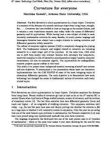
The resulting models accurately reflect their specifications and are free of unwanted wrinkles, bulges, and ripples. When the given constraints indicate and/or permit, the resulting surfaces take on the desirable shapes of spheres, cylinders, cones, and tori. Specification of a desired shape is straightforward, allowing simple or complex shapes to be described easily and compactly. For example, a “suitcase corner,” the blend of three quarter cylinders of differing radii, is formed by specifying just six sets of constraints (Fig. 1.1) plus three sets of floating vertices ( ). This work presents in detail new techniques to compute minimum variation curves, networks, and surfaces. Numerous examples demonstrating the efficacy of curvature variation as a fairness metric are provided.
1.1 Overview In this thesis, we begin with a brief outline of the techniques used to compute the various minimum variation forms. In Chapter 2, we define the terms and properties used in discussing the CAGD of curves and surfaces. In Chapter 3, we present an overview of previous work on curve, network, and surface design and computation. We describe the bulk of our work in Chapters 4, 5, and 6. These chapters are devoted to the details of the computation of minimum variation curves, networks, and surfaces respectively. Though these chapters may be read individually, each chapter builds on its predecessors. The techniques used in the computation of MVC are reapplied in the computation of MVN, and MVN themselves are used in the computation of MVS. In each of these chapters we evaluate minimum variation shapes and compare them with their contemporary 2
①
② Figure 1.1. A suitcase corner.
① specification with surface normal and curvature constraints. ② the resulting blend.
counterparts. We conclude the thesis with comments about the utility of minimization techniques, the value of curvature variation as a fairness metric, and directions for further research.
1.2 Minimum Variation Curves In CAD applications, curve design has a potentially conflicting set of requirements. Some applications demand free-form curves, along with regular curves such as circular arcs. In some instances curves must meet a set of exact positional, tangent, and/or curvature constraints. Also in general, a high degree of “fairness” is demanded of all curves. The concept of fairness is typically associated with the curvature characteristics of a curve; a fair curve has smoothly varying curvature, with as few inflections and curvature extrema as possible. The minimum variation curve (MVC) satisfies all these needs. We cast the problem of computing the MVC as a nonlinear optimization / finite element problem. The curve is broken into a series of quintic polynomial elements constructed to satisfy the given geometric constraints and join with G2 continuity. The MVC functional is minimized using a gradient descent optimization procedure. A heuristically chosen starting curve greatly accelerates convergence towards minimum variation. 3
1.3 Minimum Variation Networks Many surface modeling and data interpolation schemes use a mesh or network of curves as a key component in the construction of a smooth surface [126]. The minimum variation network (MVN) is a G2 network composed of fair curves (MVCs) that provides an excellent frame on which to build a smoothly curved surface. In fact the MVN is used in the computation of a minimum variation surface (MVS). The MVN acts either as a fixed framework on which to build an MVS or as part of the initialization step in the construction of an MVS. The MVN is computed using the MVC functional (1.1) and MVC optimization techniques with the G2 curve continuity constructions replaced by G2 surface continuity constructions. Also, the curve-based specifications are replaced by a network of surface specifications. Heuristics based on the geometry of the constraint network are used to establish a starting point for the optimization.
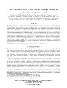
1.4 Minimum Variation Surfaces In the computer aided design of curved surfaces there is a wide range of requirements. While it is necessary to model regular shapes such as cylinders, cones, tori, and spheres, it is also important that free-form shapes can be modeled with ease. Often, it is also necessary that surfaces meet a set of exact positional, tangent, and/or curvature constraints. In all cases, surface fairness is of great importance. Like the fairness of curves, surface fairness is related to the variation of curvature across a surface; a fair surface has smoothly varying curvature. These requirements are met by MVS. As with the computation of the MVC, we compute MVS using optimization techniques to minimize the MVS functional while using constructive methods to satisfy a set of geometric interpolatory constraints. Unlike the MVC computation, MVS inter-element continuity is imposed via penalty functions. We have developed penalty functions for imposing both G1 and G2 continuity. We treat the problem of creating an MVS interpolating a collection of geometric constraints as one of scattered data interpolation. The interpolation problem is broken into three steps (Fig. 1.2); 1) connectivity definition, 2) curve network computation, 3) patch blending. In accordance with the topological type of the desired surface, the geometric constraints are first connected into a network of straight edges. Next, an MVN is calculated for the network of constraints. Finally, an MVS is computed, interpolating the MVN with at least G1 continuity. In a first approach, the boundaries of the MVS patches are fixed, interpolating the previously constructed curve network. Alternatively, the surface calculation may use the MVN as a starting point and modify its geometry during surface calculation. The latter approach yields even smoother surfaces, but at a 4
➨ ①
➨ ②
➨ ③
Figure 1.2. The blend of two pipes. Pipes are blended in three steps: ① The connectivity of the constraints is established. ② Smooth curves are fit to the constraints. ③ Surface patches are fit to the curve network.
substantially higher computational expense. The higher quality surfaces result because the curves of an MVN resulting from a given constraint set do not always lie in the MVS resulting from the same set of constraints. During the modeling process, the connectivity of the geometrical constraints is typically established as a natural outgrowth of the design process. The techniques described here are also amenable to true scattered data interpolation, in which case connectivity must first be derived with some other method, possibly based on some minimal triangulation on the data points. Our system is based on triangular and quadrilateral patches. All constraints are located at corners of these patches. Additional vertices and edges may be added to a network of constraints so that it has only three- and four-sided openings. These additional vertices are not constraints and are appropriately positioned by the curve network computation and patch blending phases of the construction. Before proceeding with a detailed discussion of these techniques, we must establish a common set of properties and terms, and review previous attempts at solving these difficult design problems.
5
6
2 Curve and Surface Terms and Properties
Minimum variation curves, networks, and surfaces are designed to solve many of the problems in CAGD. In this chapter we introduce terms and identify properties necessary for an understanding of these problems and necessary to differentiate and evaluate the many solutions found in the literature. Curves and surfaces for both design and approximation are characterized by those properties and attributes that affect their utility when applied to a particular problem. We will focus on the properties of curves and will include a discussion of surfaces only when necessary to make important distinctions between the properties of curves and surfaces. In the sections that follow we identify and define the terms associated with these characteristics: 2.1 Geometric Characterization of Curves 2.2 Geometric Characterization of Surfaces 2.4 Computational Form 2.5 Continuity 2.6 Order 2.7 Existence 2.8 Uniqueness 2.9 Sensitivity 2.10 Shape Preservation 2.11 Convex Hull Property 2.12 Linearity 2.13 Symmetry (w.r.t. ordering) 2.14 Invariance Under Transformation
7
2.15 Locality 2.16 Consistency 2.17 Versatility 2.18 Visual Appearance - Fairness
2.1 Geometric Characterization of Curves In describing the geometric character of a curve we consider four quantities: position, tangent ˆt , curvature κ , and torsion τ . For the purposes of this discussion, we will assume that our curve is described using a differentiable vector valued function, C(u) = { x(u), y(u), z(u) }
u ∈ [ a, b ] ,
(2.1)
where u is an arbitrary curve parameter with the restriction that C'(u) ≠ 0 for all u, this is called a regular parameterization. We will also assume an alternate parameterization resulting from the inversion of s(u) in equation (2.2). This results in what is called an arc length parameterization. u
s(u) =
∫
C'(u) du
(2.2)
a
Under this parameterization C'(s) = 1 everywhere. We will refer to C(u) when discussing a curve with arbitrary regular parameterization, and refer to C(s) when discussing an arc length parameterized curve. Finally, we refer to a curve that is actually the graph of a function as y = f(x) . To simplify the following discussion, we describe a sliding orthonormal coordinate system defined at each point on the curve. This trihedral frame is named the Frenet frame [52, p19]. The frame is composed of the curve’s tangent ˆt , normal nˆ , and binormal bˆ , each of which is defined as follows. The tangent ˆt(u) at a point C(u) is the direction of the curve at C(u) (Fig. 2.1). In terms of a parametric curve, the tangent is in the direction of the first derivative of the curve, ˆt(s) = C'(s) ˆt(u) =
C'(u) C'(u)
.
(2.3)
8
Figure 2.1. The Frenet Frame. The frame is made up of the curve tangent, normal, and binormal vectors. These vectors, in turn, define a set of three planes: the osculating plane, the normal plane, and the rectifying plane.
The binormal to the curve at a point C(u) is the perpendicular to the plane the curve lies in at C(u) (Fig. 2.1). The binormal is perpendicular to the first and second derivatives, bˆ (s) = C'(s) × C'' (s) bˆ (u) =
C'(u) × C'' (u) C'(u) × C'' (u)
.
(2.4)
9
The normal to the curve is perpendicular to the tangent and binormal, nˆ (s) = bˆ (s) × ˆt(s) nˆ (u) = bˆ (u) × ˆt(u) .
(2.5)
The coordinate frame we have defined spans three planes: the osculating, normal, and rectifying planes. The osculating plane is spanned by the tangent and normal, and is named for the circle it contains that “kisses” the curve (Fig. 2.1). The normal plane is spanned by the normal and binormal. The rectifying plane is spanned by the tangent and binormal, and is named for the fact that as it moves along a curve it sweeps out a rectifying developable surface. When this surface is “rolled out” flat on a plane, the curve that was used to generate it forms a straight line. The definitions of curvature and torsion are central to a discussion of a curve’s shape. Given the functions κ(s) and τ(s) a unique curve shape is defined. With respect to the coordinate frame we just defined, curvature and torsion describe the rate at which the trihedral frame rotates. These quantities are thus measures of how quickly the curve is turning or bending. Curvature is an instantaneous measure of how much the curve is bending in the osculating plane away from the tangent direction. Torsion is an instantaneous measure of how much the curve is bending away from or out of the osculating plane, n.b. a curve with τ(s) = 0 is planar. The Frenet-Serret formulas are a direct result of these definitions [52, p.19]: ˆt'(s) = κ(s)nˆ (s) ˆ (s) = τ(s)nˆ (s) b' ˆ (s) = − κ(s) ˆt(s) − τ(s)bˆ (s) . n'
(2.6)
Curvature is equal to the reciprocal of the radius of curvature. The radius of curvature is the radius of the osculating circle (Fig. 2.1). The center of the circle may also be established by finding the intersection of curve normal directions as they converge on the point C(u) . The formulas for curvature are: κ(s)nˆ (s) = C'' (s) κ(u)nˆ (u) =
( C'(u) × C'' (u) ) × C'(u) C'(u)
4
.
(2.7) 10
Note that when a curve is arc length parameterized, the second derivative is equal to curvature, because of this, the second derivative C'' (u) is often used as an approximation to curvature. Similarly, the formulas for torsion are τ(s) = − C'(s) × C''' (s) τ(u) = −
det [ C'(u), C'' (u), C''' (u) ] C'(u) × C'' (u)
2
.
(2.8)
①
② Figure 2.2. Surface Geometry.
A surface is locally characterized by directions and principal curvatures.
①
position, surface normal, and
11
②
principal
2.2 Geometric Characterization of Surfaces In describing the geometric character of a surface we consider three quantities: position, surface normal nˆ (a vector perpendicular to the tangent plane of the surface), and the principal directions eˆ 1, eˆ 2 and principal curvatures eˆ 1, eˆ 2 , (Fig. 2.2). We assume that our surface is described using a differentiable vector valued function of two variables, S(u, v) = { x(u, v), y(u, v), z(u, v) }
{ u, v } ∈ [ a, b ] ,
(2.9)
where u and v are arbitrary surface parameters with the restriction that S u(u, v) × S v(u, v) ≠ 0 for all u and v. In other words, the partial derivatives of S(u, v) must neither become colinear nor vanish. As in the discussion of curves, this is called a regular parameterization. Surfaces have no simple canonical parameterization analogous to a curve’s arc length parameterization. The normal to a surface is computed from the cross product of the first partial derivatives of the surface, nˆ =
S u(u, v) × S v(u, v) S u(u, v) × S v(u, v)
.
In order to describe the principal directions and principal curvatures of a surface, we must first define normal curvature. The normal curvature at a point on a surface in a direction specified by a surface tangent vector is determined from the intersection curve of the surface with the plane spanned by the surface normal and the given tangent vector. The principal directions, eˆ 1 and eˆ 2, and the principal curvatures, κ 1 and κ 2, at a point on a surface are the directions and magnitudes of the minimum and maximum of all possible normal curvatures at that point. The principal directions and curvatures are computed from the first and second fundamental forms from differential geometry [52], E = Su ⋅ Su F = Su ⋅ Sv G = Sv ⋅ Sv . and e = nˆ ⋅ S uuf = nˆ ⋅ S uvg = nˆ ⋅ S vv . respectively. Specifically, the principal curvatures are the eigenvalues of the curvature tensor. The expression for the curvature tensor is a 11 a 21 , a 12 a 22
(2.10) 12
where a 11 = a 12 =
fF − eG 2
a 21 =
2
a 22 =
EG − F gF − fG EG − F
eF − fE 2
EG − F . fF − gE 2
EG − F
The principal directions are the eigenvectors of (2.10) relative to the basis { S u, S v } .
2.3 Specification A key aspect of a curve is how it is defined, i.e., what information the designer must provide to fully define the curve’s shape. Two major classes of curves are interpolating curves and approximating curves. Interpolating curves are defined by a sequence of positions that the curve must pass through (Fig. 2.3①). Approximating curves do not necessarily pass through their defining points, however, the curves do reflect the shape formed by the sequence of defining control points (Fig. 2.3②).
①
interpolation point control point
control polygon
②
Figure 2.3. Interpolating and Approximating Curve. An interpolating curve passes through its defining points. An approximating curve passes near or through its defining control points. The collection of line segments connecting the control points is referred to as the control polygon.
Curves shapes based on user provided positions represent the simplest form of specification. Implicit in the specification of a sequence of points is their ordering; a curve designer may also be required to specify the parametric spacing of the points along the curve, their parameterization. In addition to interpolated points, curve definitions may 13
Figure 2.4. An Interpolating Curve. A curve specified by its end positions, tangent directions, and one curvature value.
include higher order geometric specifications such as tangent direction, curvature, and torsion (Fig. 2.4). Curves may also be defined by positions augmented with parametric derivatives, with respect to the independent curve parameter. Such specifications concern the method used to represent the curve rather than the intrinsic geometry of the curve. Finally, curves may have associated shape handles, parameters which are neither geometric nor parametric in nature, but control the shape of the curve in a predictable fashion. Tension [193] is a typical shape handle, an increase in tension causes the curve to decrease in fullness, as though the curve were being pulled more tightly to its defining control polygon (Fig. 2.5).
2.4 Computational Form Curves may be represented and computed using a variety of techniques and forms. The three basic forms are implicit, parametric, and explicit. For example, a unit circle centered at the origin may be defined in each of these forms. 1.
Implicit: 2
2
x +y −1 = 0 2.
The implicit form is particularly useful for point classification (determining whether a point is inside, on, or outside a closed curve). In general, there is no direct method for computing a sequence of points that lie on an implicit curve.
3.
Explicit:
y = 1−x
2 2
y = − 1−x −1 ≤ x ≤ 1 4.
The explicit form, the simplest of curve forms, is useful for curves representing functions. In the case of the circle, two separate equations are required because it is multi-valued. The explicit form is commonly used in the approximation of functional data.
14
①
② ③
④
Figure 2.5. Increasing Tension in a Curve. Tension is varied from a low value (①, ③) to a high value (②, ④) causing the curve to follow its defining control polygon more closely. (①,②) interpolating curve, (③, ④) approximating curve.
5.
Parametric:
x = sin u y = cos u −π ≤ u ≤ π
6.
x= or
y=
2
1−u
2
1+u 2u
2
1+u −∞ ≤ u ≤ ∞
Finally, the parametric form, sometimes referred to as vector-valued, provides a simple mechanism for the representation of curves. Points on the curve are computed as a vector valued function of an independent parameter. Because of their flexibility and the ease with which sequences of points on a curve may be calculated, the parametric form has emerged as the favored approach for CAD applications.
Curves may be further classified by the type of functions which they employ. Parametric curves are defined using polynomial, rational polynomial, trigonometric, and exponential functions. Polynomial and rational polynomial functions are preferred because of the ease with which they may be computed, only requiring the elementary operations on real numbers, addition and multiplication for plain polynomials, and division for rational polynomials. Further, polynomials are easily differentiated, and at least theoretically, may always be symbolically integrated. 15
Finally, curve generation techniques may be classified based on their ability to interpolate or approximate multi-valued data. A curve that only supports function interpolation and approximation is referred to as single-valued (Fig. 2.6). Function interpolants are single-valued, while curve interpolants can be multi-valued.
C(u)
f(t)
f(t)
multi-valued curve
single-valued curve
t
Figure 2.6. Multi- and single-valued curves.
2.5 Continuity Because of the limited descriptive power of a single parametric polynomial, multiple parametric polynomials may have to be pieced together to form a more complicated curve. The resulting curve is referred to as piecewise polynomial. In order to provide guarantees concerning the smoothness of such a composite curve, the notion of continuity has been introduced. Continuity refers to the smoothness of the joints between adjacent polynomial pieces. Consider the piecewise polynomial curve that is globally parameterized from 0 to 3 (Fig. 2.7). The curve is made up of three polynomial pieces or segments. In order for the curve to be considered to be first order parameter continuous (C1), the first derivatives of the segments must be equal at the joints: c' 0(1) = c' 1(0)
and
c' 1(1) = c' 2(0) .
(2.11)
In order for the curve to be second order parameter continuous (C2), both the first and second derivatives have to be equal: c' 0(1) = c' 1(0) c'' 0(1) = c'' 1(0)
c' 1(1) = c' 2(0) c'' 1(1) = c'' 2(0) .
(2.12) 16
c 0(u) = C(u) 0 ≤ u ≤ 1
C(2)
c' 0(1) = c' 1(0) C(1)
C(3) c 1(u − 1) = C(u) 1 ≤ u ≤ 2 c' 1(1) = c' 2(0)
C(0)
c 2(u − 2) = C(u) 2 ≤ u ≤ 3
C(u) 0 ≤ u ≤ 3
Figure 2.7. A C1 Piecewise Parametric Curve. Curve segments join so that the first derivatives are equal at the segment-segment joints.
Similarly, to achieve nth order parameter continuity (Cn), the first n derivatives of the curve segments must be continuous at the segment-segment joints. For a complete discussion of curve and surface continuity see [47]. A less restrictive form of continuity is that of geometric continuity, denoted Gn for nth order geometric continuity. It stipulates that curve segments can be made to meet with parametric continuity under some suitably chosen parameterization, i.e., it must be possible to reparameterize adjacent segments such that they meet with parametric continuity. Examining the case of G1 continuity, unit tangent vector continuity is necessary and sufficient for first order geometric continuity to be achieved. For G2 continuity, the curve segments must have the same curvature at the junction in addition to tangent continuity. A result of geometric continuity is the availability of extra degrees of freedom which are useful for controlling curve shape. Consider a curve made up of cubic Hermite segments. A cubic Hermite segment [59] is specified by the positions and first parametric derivatives at its end points, c i(0), c i(1), c' i(0), c' i(1) . To form a C1 continuous curve, the positions and first derivatives must be explicitly shared at segment-segment joints. To form a G1 continuous curve it is only necessary that the segments share tangent direction, ˆt i(u) , at these joints (Fig. 2.8). To accomplish this and to take advantage of all the available degrees of freedom, we redefine the cubic Hermite segment to be defined by the positions, tangent directions, and first derivative magnitudes at its end points, c i(0), c i(1), ˆt i(0), ˆt i(1), m i(0), m i(1) .
(2.13)
17
C(2) C(1)
C(3) C(u) 0 ≤ u ≤ 3
C(0)
ˆt i(u) =
c' i(u) c' i(u)
c 0(u) = C(u) 0 ≤ u ≤ 1 ˆt 0(1) = ˆt 1(0) c 1(u − 1) = C(u) 1 ≤ u ≤ 2 ˆt 1(1) = ˆt 2(0) c 2(u − 2) = C(u) 2 ≤ u ≤ 3
Figure 2.8. A G1 Piecewise Parametric Curve. Curve segments join such that the tangent directions are equal at the segment-segment joints.
To map to the traditional Hermite form, we scale the tangent direction by the associated magnitude producing the appropriate derivative, c' i(0) = m i(0)tˆi(0)
c' i(1) = m i(1)tˆi(1) .
(2.14)
The use of geometric continuity has produced two extra degrees of freedom per curve segment, m i(0), m i(1) . These degrees of freedom may be used as shape handles to further control the shape of the curve without losing geometric continuity. As a more concrete measure of the descriptive power of curves exhibiting geometric versus parametric continuity, we examined the relative degree of the parametrically continuous curve required to exactly reproduce a geometrically continuous curve. We found that a degree dk, Ck curve is required to reproduce the shape of a degree d, Gk curve. Consider a Gk curve composed of curve segments C 0…n(u) , we may assume without loss of generality that each segment is parameterized with u ∈ [ 0, 1 ] . Starting at the first
18
joint, between C 0(u) and C 1(u) , we fix the parameterization of the first segment and reparameterize the second (producing C' 1(u) ) such that their derivatives match at the joint where they meet: ( 1)
( 1)
( 2)
( 2)
C 0 (1) = C' 1 (0) C 0 (1) = C' 1 (0) … ( k)
( k)
C 0 (1) = C' 1 (0) The required reparameterization is of the form k
u =
∑ βi u' i ;
(2.15)
i=1
u is replaced by a degree k polynomial in u' , the parameter of the reparameterized curve. Since C 1(u) is a degree d polynomial, replacing u with a degree k polynomial, creates a degree dk polynomial, C' 1(u') . The coefficients of (2.15) are calculated by making the substitution and differentiating C 1(u') ; ( 1)
( 1)
( 2)
( 2)
( 3)
( 3)
C 0 (1) = β 1 C 1 (0) ( 1)
C 0 (1) = β 21 C 1 (0) + 2β 2 C 1 (0) ( 1)
( 2)
C 0 (1) = β 31 C 1 (0) + 6β 1 β 2 C 1 (0) + 6β 3 C 1 (0)
(2.16)
… Using this system of equations, the β i are easily found. Since C' 1(u') is reparameterized, k i β i x . Continuity between segments C' 1(u') the range of u' is now 0…x, where 1 = i=1 and C 2(u) is similarly established
∑
( 1)
( 1)
( 2)
( 2)
( 3)
( 3)
C' 1 (x) = β 1 C 2 (0) ( 1)
C' 1 (x) = β 21 C 2 (0) + 2β 2 C 2 (0) ( 1)
( 2)
C' 1 (x) = β 31 C 2 (0) + 6β 1 β 2 C 2 (0) + 6β 3 C 2 (0) … 19
(2.17)
Continuing this process creates a series of curve segments that meet with Ck parametric continuity and which are each parameterized from 0…x i . A single unified parameterization can be established by further substitution without affecting the degree of the result. Schoenberg [191] introduces a specific instance of a piecewise polynomial function, the spline. While his definition is of a scalar spline function used for approximation, we consider a vector valued spline curve: U = ( u o, u 1, …, u n )
u i ∈ ℜ, u i ≤ u i + 1, i = 0, …, n − 1
(2.18)
U is called a knot vector and is composed of knot values u i . A vector valued function C(u) of degree d is a spline function if it satisfies two conditions. First, the segments C i(u) of which it is composed, are each parameterized u ∈ [ u i, u i + 1 ] , and are polynomials of degree d. Second, C(u) and its derivatives C'(u), C'' (u), …, C
( d − 1)
(u) are continuous,
d−1
. The notion of a spline curve is used extensively in curve design and has C(u) ∈ C become somewhat less strictly defined as a curve composed of C∞ segments meeting with specified continuity, either parametric or geometric.
2.6 Order Order refers to two distinct characteristics of a curve. First, when referring to a polynomial or rational polynomial representation, the order of a curve refers to the order of the polynomials employed. When speaking about rational polynomials, the orders of the numerator and denominator need not be equal and thus both are stated. Order is the number of degrees of freedom in a scalar-valued polynomial, thus it is one greater than degree; a quintic polynomial is sixth order. Second, order also refers to the accuracy of an interpolation technique. The order of interpolation is the maximum order of a polynomial that is exactly recreated from sampled data. The order of convergence refers to the rate at which an approximating curve converges on an analytic curve as the number of samples is increased.
2.7 Existence The question of existence of a solution to a problem is widely studied. In the context of curve design, the question of existence is whether or not a curve generation technique or algorithm produces a desired result for all input specifications, for only some inputs, or for no inputs at all. Alternatively, the question may be whether the curve generated is useful, e.g. is the solution curve of finite length? Most work on formal proof of existence is in the 20
area of solving differential equations. For most constructive curve generation techniques existence is easily proved, or it is possible to characterize the necessary and sufficient restrictions on inputs for solutions to exist. In some cases existence may be conditional on the representation used; a differentiable curve may exist that meets the curve specification, but that curve may not be in the space of curves covered by the representation used. Existence proofs for curve generation techniques using iterative methods such as functional minimization require the derivation of characteristic differential equations and their subsequent analysis. Correctly characterizing a system based on functional minimization with all its associated constraints is extremely complex, and proof of existence is difficult or even impossible. In the absence of an existence proof, it may still be possible to heuristically identify configurations that lead to unusable solutions, e.g. a solution curve of infinite length. For example, a minimum energy curve (MEC, (3.1.1)) will run off to infinite length if the angular difference between supports is greater than π (Fig. 2.9). In order to guarantee that an MEC exists for a given interpolation problem, the arc length of the curve must be limited. The necessity of this restriction is pointed out by Birkhoff and deBoor [13] who observe that a “satisfactory” interpolant composed of circles of infinite radius may be constructed to solve any interpolation problem while consuming zero energy. Jerome [104] established the sufficiency of limiting the arc length of the solution curve.
∞
∞
1.
0.5
-1.
-0.5
0.5
1.
①
② Figure 2.9. A Minimum Energy Curve.
① the curve resulting from clamping end points with tangent directions ② the curve where the difference in tangent directions is ε greater than π.
21
differing by π.
2.8 Uniqueness Once the existence of a solution to a curve generation problem has been established (empirically or otherwise), it may be desirable to find out if there is more than one solution to the problem as stated. Again, constructive curve generation techniques normally result in the calculation of a single curve. Curves based on functional minimization often have multiple solutions which represent multiple local minima in the energy landscape. It is often insufficient to characterize the unique solution as that curve for which the functional is globally minimized. Because in fact, in many cases, the global minimum is not the desired minimum, e.g. the global minimum of an MEC is a curve of infinite length. If a unique solution does not exist, it is normally necessary to modify the functional, to add extra conditions, to change the approach used in calculating the curve, or some combination of these. In the case of the MEC, the continuum method (described below) can be used to compute a locally unique solution. The continuum method is a technique where a continuous family of solutions is found and the desired solution is normally found at one end of the continuum. We start our continuum with an MEC limited in arc length to the accumulated chord length of the sequence of points connected one to the next. The continuum is formed by gradually relaxing the arc length constraint until a stable configuration or an upper arc length bound is reached. A stable configuration is a curve shape that is a local minimum of the original MEC functional, free of arc length constraints.
2.9 Sensitivity The sensitivity of a curve generation technique refers to how a curve’s shape varies with its defining data and even the algorithm used to compute its shape. First, is the derived solution sensitive to the starting point? This applies primarily to curves computed using iterative techniques such as minimization and is closely related to the issue of uniqueness. Second, if the specification of a curve is modified continuously, does the solution vary continuously? Figure 2.9 is an example of high sensitivity to small change, the specification of curve ① is modified by ε and curve ② results, a curve of infinite length. Finally, does a small change in specification lead to a small change in solution? During interactive design, it is important that a curve’s shape respond in a reasonable and controllable fashion to a user’s actions. A minor modification to a curve’s specification should not result in a gross change in shape.
22
2.10Shape Preservation Shape preservation is that aspect of a curve technique which determines how faithfully it reproduces the shape of its defining data. For example, consider a curve defined by interpolation points that vary monotonically in some direction, e.g. non-decreasing x and y. If the curve resulting from monotonically varying points is also monotonic then the curve is said to preserve monotonicity (Fig. 2.10). Similarly, convexity preservation states that if the points defining a curve form a convex path then a convexity preserving curve must also remain convex (Fig. 2.11). Restated, a convexity preserving curve may have no more inflection points than its defining control polygon.
not monotonicity preserving
monotonic data
monotonicity preserving Figure 2.10. Monotonicity Preservation. Two curves are fit to monotonically varying data points. The upper curve does not preserve monotonicity. The lower curve is non-decreasing preserving the monotonicity of the data.
An even stronger property than convexity preservation and monotonicity preservation is the variation diminishing property[191]. It states that a curve does not oscillate more often about any straight line than the piecewise linear interpolation of the data points. An 23
①
②
③
Figure 2.11. Convexity Preservation. Two curves are fit to data points which are convex ①, i.e. the control polygon has no inflections. Curve ② has inflection points and thus is not convexity preserving. Curve ③ has no inflections, accurately reflecting the data and thus is convexity preserving.
alternative statement of the property is that no straight line should intersect the generated curve a greater number of times than it intersects the curve’s control polygon. A variation diminishing curve is always smoother than the data used to define it (Fig. 2.12).
①
② Figure 2.12. Variation Diminishing Curve.
Curve ① smooths the associated defining data, where curve ② does not. There is no line which intersects curve ① a larger number of times than it intersects the control polygon.
24
2.11 Convex Hull Property The convex hull property states that a curve remains within the convex hull of its defining points (Fig. 2.13①). Note that this property also only applies to approximating curves because interpolating curves must go outside the control hull. In Figure 2.13② we see the broader definition of the convex hull property. Here a piecewise quadratic curve remains within the union of the convex hulls of the points taken three at a time. Similarly, if the curve were composed of cubic segments the curve would remain within the union of the convex hulls of the points taken four at a time.
①
② Figure 2.13. The Convex Hull Property.
①
the curve remains within the convex hull of its defining control points. ② a piecewise quadratic curve remains within the union of the convex hulls computed three points at a time.
2.12Linearity Consider a technique for creating curves that takes as input a series of points p i and produces a curve C p(u) that is swept out by varying the curve parameter u. The technique used to create C pi(u) is considered to be linear if the following identity holds for all inputs: C pi + qi(u) = C p(u) + C qi(u) .
25
2.13Symmetry (w.r.t. ordering) Curves defined by sequences of points may be sensitive to the order in which the points are processed. A curve fitting technique is symmetric if the order in which the points are processed has no effect on the shape of the resulting curve, i.e. a curved shape defined by points p 0 …p n should be equivalent to the shape defined by points p n …p 0 [24].
2.14Invariance Under Transformation Invariance under transformation means that a curve should not change shape under a change of the coordinate system in which the data is described. Furthermore, under certain transformations of the data, the resulting shape may change in a simple predictable manner. Considering a transformation T applied to the data defining a curve and to the curve itself if these produce the same curve: T ⋅ C(p i, t) = C(T ⋅ p i, t) ,
(2.19)
then the curve is said to be invariant under that transformation. There are three types of transformational invariance of particular interest: invariance under similarity transformations, invariance under affine transformations, and invariance under affine parameter transformations. First, let us describe a hierarchy of transformations in terms of the geometric measures they preserve. Rigid body motions preserve both angular and length measures. Similarity transformations augment rigid body motions with uniform changes of scale; angular measures and ratios of lengths are preserved. Finally, affine transformations preserve parallel lines, and the ratios of lengths of parallel lines. We start by considering function interpolation and approximation. The curve fit to data from a function should not change shape if the units of measure are changed, i.e. it should not change shape if scaling is performed along the axes (nonuniform scaling.) It is generally not required that function interpolators exhibit transformational invariance under anything more than nonuniform scaling. Curve modeling techniques used in CAD applications should exhibit invariance under similarity transformations. It should be possible to apply modeling transformations (e.g. rotation, scaling, etc.) to a curve without the curve changing shape. There are curve methods that are invariant under affine transformations, such invariance is not a prerequisite for CAD utility, in fact it is not always desirable behavior (Fig. 2.14). In Figure 2.14① affine invariance and a nonuniform scaling results in exaggerated overshoot. In Figure 2.14② a similar nonuniform scaling results in an oval curve where a circular curve is appropriate. 26
①
original
not affine invariant
affine invariant
②
original
not affine invariant
affine invariant
Figure 2.14. The Effect of Affine Invariance.
①
demonstrates overshoot as a result of affine invariance. ② demonstrates compression as a consequence of affine invariance.
2.15Locality Consider a curve defined to interpolate a series of points, if the movement of a single point changes the shape of the entire curve then the technique used to generate the curve exhibits no locality whatsoever and is considered global. Locality refers to the extent that one part of a specification is limited to affect only a small, well defined portion of a curve. For example, if a single point to be interpolated is moved, how does the resulting curve change shape? If a curve’s shape only changes in the neighborhood of the relocated point, then the technique exhibits local behavior (Fig. 2.15). For an interactive design process it is very important to have control over the locality of modification. A designer may become frustrated if a modification at one end of a curve resulted in an unexpected change 27
①
②
③ Figure 2.15. Local vs. Global control. The central point of a curve ① is moved. The curve resulting from the technique exhibiting local control ② only changes shape in those spans adjacent to the relocated point. The curve resulting from a global technique ③ changes throughout in response to the modification.
at the other end of the curve. Pseudo-local control is exhibited by techniques where relocation of a control point causes a formally global change in the curve definition, but the apparent change is quickly attenuated as the curve leaves the neighborhood of the modification. On the other hand, it is also desirable to allow larger scale modifications to a curve’s shape; e.g. a curve with fine detail might require global bending. We refer to those techniques which provide explicit control over the locality of changes as having variable locality.
2.16Consistency The concept of consistency refers to a characteristic of interpolation techniques. In both function and curve interpolation a consistent technique is one that preserves the shape of a curve when an interpolation problem is augmented with additional constraints or data points that match the geometry of the curve. In Figure 2.16① we see an original curve, defined by six positional constraints. In Figure 2.16②,③ we see two possible results of adding an additional positional constraint, i.e., a point lying exactly on the curve. In ②, an 28
add a point already on the curve ②
①
inconsistent
③
consistent Figure 2.16. Consistency. Consistency is the property that a curve’s shape remains unchanged when a compatible constraint is added to an interpolation problem.
inconsistent technique produces a curve of modified shape. In ③, precisely the same curve is produced. The concept of consistency is most often achieved by techniques which, by some measure, produce the best curve possible under the given constraints. If a new best curve were produced by the addition of a new point on the curve then the previous “best” curve was apparently not the best—a contradiction!
2.17Versatility In section 2.4 we described the various computational forms that are used to describe curves. Another aspect of curves and the techniques used to generate them is their inherent versatility. As we have seen, some curve techniques are only capable of modeling single-valued curves, while others may be multi-valued. In addition, some techniques may only be applicable to planar curves, while others may model space curves with piecewise planar segments, while still others may be true space curves. For example, a quadratic 29
curve is by definition a planar curve. The versatility of a curve technique is also determined by what types of curves can be represented exactly. For example, circular and elliptical arcs can only be approximated by polynomial curves, whereas rational polynomial curves may exactly model conic sections.
2.18Visual Appearance - Fairness The inherent subjectivity of assessing the appearance of a curve makes the definition of pleasing appearance and fairness difficult. The difficulty of arriving at a definition is compounded by the fact that it is application specific. Despite, or perhaps because of this, a number of definitions have been put forth. A curve’s shape is completely described by the curve’s curvature and torsion as they vary along its length. For plane curves this may be reduced to curvature because torsion is zero. From this observation it should not be surprising that most quantitative measures of curve quality are stated in terms of curvature and sometimes torsion. The earliest discussion of fairness this author has found predates CAD and curve design by many years. In Aesthetic Measure [15], George Birkhoff provides quantitative analysis of various art forms: polygonal forms, ornaments and tilings, vases, music and poetry. It is in the section concerning vases that he describes the “Requirements for Regularity of Contour”. This discussion of the curvature of the outline of a vase remains a preeminent definition of fairness: “The following further consideration of the requirements for regularity of contour is to be regarded as tentative. It is clear that such requirements can never be given any very satisfactory formulation. Consider a convex curve made up of arcs of circles of different radii, tangent to one another at their common end points. Evidently the impression produced is not that of a single unified curve, especially if the radii are alternately larger and smaller. A first obvious requirement, therefore, is that the curvature varies gradually (that is, continuously) along the curve and oscillates as few times as possible in view of the prescribed characteristic points and tangents. In particular the curvature should not oscillate more than once on any arc of the contour not containing a point of inflection. By inspection of various vase forms like those shown later, it is found that this condition is satisfied in practice. A second requirement is that the maximum rate of change of curvature be as small as possible along the contour. This condition eliminates both unnecessarily large curvatures along the contour and unnecessarily rapid changes in curvature. Although the strict application of these two conditions would be very difficult, still they may be regarded as substantially satisfied when it is not feasible to modify the curve so as to diminish either the greatest curvature or the rapidity of change of curvature. The curves of contour actually employed will be found not to permit of such modification.
30
The eye can follow with ease curves meeting these two requirements, just because of the small curvature and its small rate of change.”
As mentioned above there are many definitions of fairness; some other definitions of fairness are paraphrased below: A curve is fair if its curvature plot is continuous and consists of only a few monotone pieces [59]. 2. “A frequency analysis of the radius of curvature plotted against arc length might give some measure of fairness, the lower the dominant frequency, the fairer the curve [M. Sabin from 70]. 3. A fair curve has minimum strain energy [180]. 4. A curve is “fair” if it can be drawn with a small number of french curve segments [56]. 5. A curve’s curvature plot must be almost piecewise linear, with only a small number of segments. Continuity of curvature is an obvious additional requirement [56]. 6. The curve should be convexity preserving [202]. 7. A curve is characterized as fair if its curvature plot is continuous, has the appropriate sign (if the convexity of the curve is prescribed), and it is as close as possible to a piecewise monotone function with as few monotone pieces as possible [187]. 8. Fairness is measured as the integral of the square of the second derivative of the curve [146]. 9. In many design applications a gentle, gradual development of curvature along a curve is much desired and is often used as a subjective measure of curve fairness [135]. 10. A curve is fair if its curvature plot consists of relatively few monotone pieces [57]. 11. The properties desired of a fair curve are smoothness, shape preservation, absence of extraneous inflection points and the like, but a curve which satisfies all of these criteria as well as the original constrains may still fail to be fair.... Fairness measures must depend only on the geometric invariants of the curve and be independent of the curve’s parametrization. A curve’s shape should minimize either the variation of the radius of curvature or the variation of curvature [182]. 12. A plane curve is called fair if the following three conditions are satisfied: (1) The curve is G2; (2) There are no unwanted inflection points on the curve; (3) The curvature of the curve varies in an even manner. Expanding on (3): (i) The number of extreme points of the curvature should be as small as possible. (ii) The curvature of the curve between two adjacent extreme points should vary almost linearly [27]. 1.
These definitions, in particular Birkhoff’s, point to the approaches we have taken. Birkhoff suggests minimizing the maximum curvature, and minimizing the variation of curvature overall.
31
32
3 An Abridged History of Curve, Network, and Surface Design
To better understand the problems encountered in free-form shape design, we review the approaches that have been developed for curve, network, and surface design.
3.1 Curves and Curve Design Much of the work on curve design has been to develop methods that behave naturally in response to user specifications. A great deal of work has been devoted to the mathematical modeling of the draftman’s spline. A draftman’s spline is a thin, smoothly bending strip of wood held in place by weights called ducks (Fig. 3.1). The first recorded work related to physical splines dates to the 18th century, to a study of elastica by James and Daniel Bernoulli, and Leonhard Euler. Elastica are idealized thin beams. The Bernoulli brothers postulated that the work required to bend a thin beam was proportional to the square of the curvature. In a letter to Euler, Daniel Bernoulli suggested that the shape of the elastica was such that its squared curvature was minimized. Acting on this suggestion Euler derived the differential equation of the curve and classified its forms [124].
33
Figure 3.1. Draftman’s Spline and Ducks.
In 1946, Schoenberg introduced the polynomial spline function, a piecewise polynomial function of degree n whose segments meet with Cn-1 parametric continuity. In 1957, Holladay introduced the cubic spline for function interpolation and integration. The curve he developed minimized
∫
2
2
d f(x) dx . 2 dx
(3.1)
He noted that for curves with modest slopes, f '(t) « 1 the cubic spline provided a good approximation to the bending of a thin rod. It is at this point that the development of curves and curve design techniques branches, with one vein of work building on the cubic spline and the other continuing to pursue improved approximations of elastica and other physical approaches. Since the latter branch is more closely related to MVC, we will first review that work, and return to the cubic spline and its descendants in section 3.1.2. The remainder of this section is broken down topically as follows: 3.1.1Nonlinear Splines: Elastica, MEC, Physically Based Curves, MVC 3.1.2Interpolating Splines: The Cubic Spline and its Descendants 3.1.3Local Interpolation Methods 3.1.4Bézier Curves and Composition Constructions 3.1.5Shape Preserving Splines 3.1.6Intrinsic Splines 3.1.7Local Approximating Splines: The B-spline and its Descendants 3.1.8Variable Locality 3.1.9Surveys
34
These subsections represent a survey of work on curve design and we provide them to illuminate the prevalent problems in CAGD.
3.1.1 Nonlinear Splines: Elastica, MEC, Physically Based Curves, MVC Minimum energy curves, minimum variation curves, and other members of this family require the solution of systems of nonlinear equations in order to compute their shape, thus their classification as nonlinear splines. Even Mehlum [132] developed a technique for generating an approximating curve based on a spring model using the calculus of variations. In this model, the curve was suspended by springs attaching the curve to its control points (Fig. 3.2).
Figure 3.2. A Spring Curve. An approximating curve is calculated by simulating the effect of springs attaching a rod to a series of anchors or control points.
Birkhoff et al. [14] presented a theoretical comparison of nonlinear mechanical splines, elastica, and Wilson-Fowler splines (Fig. 3.3), discussing possible methods for the computation of mechanical splines and elastica. The mechanical spline is a model of a thin beam passing through frictionless, swiveling supports; it is a special case of the elastica in which no tangential forces act on the beam or curve. Glass [78] presents the first algorithm to compute mechanical splines or minimum energy curves (MEC) as they have become widely known. His algorithm uses numerical techniques to compute discrete points on the 35
curve. Mehlum [133] developed techniques for the computation of MEC, producing a piecewise circular arc approximation of arbitrary precision. Mehlum uses these methods in the Autokon system for curve and surface design [131]. Woodford [211] improved on Glass’s algorithm for computing discrete MEC. Lee and Forsythe [118] discuss the variational and differential properties of open and closed MEC. Malcolm [125] further improves the computation of discrete MEC. Jerome [104] discusses the necessary and sufficient conditions for the existence of a minimum energy curve. Fischer and Jerome [65] discuss the stable and unstable equilibrium of MEC. Stable equilibrium of MEC refer to local minima of the energy functional, a configuration where the curve holds its shape with no constraint on its arc length. Golomb and Jerome [79] present theoretical results establishing conditions for equilibria, uniqueness, and regularity. Horn [101] thoroughly studies a specific MEC segment, defined by two points on a baseline with a vertical tangent constraint specified at each point. The resulting curve resembles a croquet hoop. Horn computes closed form expressions for the energy, arc length and maximum curvature of his subject curve. Ohlin [149, 150] introduces the concept of consistency (2.16) and discusses consistent interpolation methods. He finds that, given requirements of second order continuity, invariance under similarity transformations, and consistency, there are very few acceptable interpolation methods. For function interpolation, Holladay’s cubic spline is the only consistent solution. For curve interpolation, the available methods belong to a continuous family of curves that include MEC, a Cornu spiral1, and the lemniscate. Independently he developed a fourth order continuous consistent spline that minimizes the arc length integral of the square of the arc length derivative of curvature, the MVC. Ohlin presents an algorithm for the computation of an MVC segment specified by position, tangent, and curvature at the end points. His algorithm computes discrete positions, tangents, and curvatures on the MVC and fits them with a piecewise quintic polynomial curve. Ohlin also outlines the advantages of MVC over MEC:
1
1.
higher order continuity.
2.
it caters to our human preference for circles.
3.
curvatures at the extreme points may be estimated by the splining method, as well as the directions. (sic)
4.
curvature and/or directions can be prescribed at all points, end points or interval, without losing continuity of curvature.
5.
demanding to keep curvature as constant as possible rather than as small as possible will reduce the likelihood of undesired changes of sign in curvature.
6.
as we have seen before, a stable solution to MEC does not always exist.
A Cornu spiral is a curve with linearly varying curvature. Also known as Euler spiral, linarc, lince, and clothoid.
36
Kallay [114] describes a method based on finite sums and discrete optimization to compute the MEC in ℜ3 of fixed arc length. Jou and Han [111, 112] discuss the calculation of discrete MEC subject to arc length and tangent constraints. In his thesis, Tom Rando [178] discusses the application of optimization to Bézier curve and surface design. With respect to curve design, he minimizes the arc length of the evolute of a curve segment specified by position, tangent, and curvature at the end points. This amounts to minimizing the arc length derivative of the radius of curvature, 2
1 d κ(s) ds . ds 0 l
∫
(3.2)
He also mentions the possibility of minimizing the arc length derivative of curvature, the MVC functional. Finally, Celniker and Gossard [31] describe an interactive design system based on modeling curves and surfaces using physical simulation. The system uses finite element methods to compute the shape of curves subject to position and tangent constraints. The resulting curves converge on the MEC as the number of elements used is increased. The line of work traced out in this section reflects a search for an optimal/ideal interpolant. This search began in a largely theoretical realm, ending in the application of these concepts in an interactive environment. As a further testament to the potential of these methods, Forrest [71] remarks that Autokon [131] is generally successful in producing curves acceptable to naval architects, aerodynamicists, and car stylists, from relatively crude data. Our work continues and parallels this vein; due to the increased speed of workstations, better solutions to interpolation and design problems are now possible.
3.1.2 Interpolating Splines: The Cubic Spline and its Descendants As mentioned in the introduction to section 3.1 on page 33, the cubic spline was introduced by Holladay as an approximation of the MEC. The work following his introduction concerned methods for achieving an improved approximation to the MEC and reducing or eliminating the unwanted wiggles or oscillations sometimes observed in cubic splines. First, Asker [5] introduces several approaches that seem to have been lost or overlooked by later researchers. First Asker introduces a method allowing the stiffness of the spline to be varied along its length. This scheme provides a method to overcome 37
wiggles. Two versions of variable stiffness are presented. First, stiffness varying in a piecewise constant fashion results in a C1 cubic spline. And second, stiffness varying in a piecewise linear fashion results in a C2 quartic spline. These methods are equivalent to the weighted spline of Salkauskas [186]. The second approach involves the establishment of a local coordinate system between adjacent interpolation points (Fig. 3.3). This curve has since become known as the Wilson-Fowler spline [77] and is used heavily by the DoE. The approach is designed to locally reduce the magnitude of y'(x) thereby improving the approximation to the MEC. The Wilson-Fowler spline requires the iterative solution of a nonlinear system of equations. In addition to improving the approximation to the MEC, the Wilson-Fowler spline allows for the interpolation of multi-valued data sets, whereas cubic spline function interpolation is limited to single-valued curves.
y y x x y
x
y ( x)
is cubic
Figure 3.3. The Wilson-Fowler Spline. Local coordinate systems are formed at each interpolation point of the Wilson-Fowler spline. The x axis of the coordinate system is aligned with the chord connecting adjacent points, the y axis is perpendicular to the chord.
Ferguson [64] introduces the parametric cubic spline curve by applying cubic spline function interpolation to vector valued data. A multi-valued curve defined by x, y, [ z ] , u , where x, y, z specify the Euclidean space coordinates of the interpolation point and u is the independent curve parameter. The value of u specifies the location of the interpolation point in the parameter space of the spline. This is analogous to the role of the x-coordinate in function interpolation. Note that the sequence of u i must be nondecreasing.
38
Schweikert [193] introduces the spline under tension as a means to deal with the spurious oscillations sometimes observed in cubic splines. The solution to the system he set up results in a curve described by exponential functions. Cline [37], and Pilcher [163] further develop splines under tension. In part due to the expense of computing these exponential curves, Nielson [140] introduces the ν -spline as a C1 piecewise cubic polynomial alternative to splines in tension. In addition to providing a similar tension parameter, ν -splines extend splines in tension by allowing tension to vary along the curve affording greater control over curve shape. Hagen [94] introduced the τ -spline as a generalization of the ν -spline; a piecewise quintic exhibiting G2 continuity. Later, Foley [69] introduced the cubic weighted ν -spline, a generalization of C2 cubic splines, weighted splines, and ν -splines. Extending piecewise polynomial splines in another direction, Meier and Nowacki [135] describe splines that minimize:
∫
2
∫
f '''(t) dt (jerk or shear) and f
( 4)
2
(t) dt (load).
(3.3)
The result is a smoother, higher degree interpolant; note that “jerk” approximates the derivative of curvature, and minimizing it approximates an MVC. Similarly, Pottmann [167] extends τ -splines adding a third derivative term to the functional for minimization. Pottmann’s spline results in a G3 continuous interpolant, with G4 continuity achievable with uniform tension. Thus far, the works discussed have introduced shape handles and increased continuity. We now discuss some methods for the automatic setting of shape parameters and for the automatic parameterization of spline curves; parameterization is an additional means of shape control. First, consider the problem of parameterization. There are several methods in wide use for establishing the parameterization of a cubic spline. The two simplest are uniform parameterization and chord length parameterization. Using uniform parameterization, interpolation points fall at evenly spaced parameter values. Chord length parameterization stipulates that the points be spaced parametrically relative to the Euclidean distances between successive points (Fig. 3.4). Marin [128] describes a parameterization technique that minimizes an objective function. The resulting parameterizations reduce overshoot, lower C3 discontinuities, and center oscillations in the second derivative around zero. The solution is calculated in closed form for the case of cubic function interpolation; unfortunately, the solution is only calculated as a numerical approximation in curve interpolation problems. Farin [59:130-134] outlines other methods for determining improved parameterizations. 39
u1 = 1 u2 = 2
u0 = 0
u4 = 4
u3 = 3
u5 = 5
u1 = 5 u2 = 9
u0 = 0
uniform parameterization
u 4 = 24
u 5 = 29
u 3 = 14
chord length parameterization
Figure 3.4. Uniform vs. Chord Length Parameterization. A cubic spline is fit to data using uniform and chord length parameterizations. The chord length parameterized curve is smoother than the uniformly parameterized curve.
Methods for automatically setting shape handles are less well developed. The setting of shape handles is typically done interactively by the user/designer. Schweikert [193] discusses conditions necessary for the absence of unwanted inflections, and provides an explicit formula for setting the tension parameter of a uniformly parameterized cubic spline to satisfy these conditions. Fletcher and McAllister [67] describe an algorithm for automatically setting the tensions of a cubic spline function interpolant to remove unwanted oscillations. Other methods for automatic shape preservations are reviewed in section 3.1.5.
3.1.3 Local Interpolation Methods Thus far we have described global methods for computing interpolating curves. In this section we review local methods for computing smooth interpolating curves. Using local methods, curves are typically less computationally expensive to calculate, and because local methods exhibit local control, the resulting curves can be easier to manipulate during the interactive design process. It is also possible to identify special configurations of control points which can then receive treatment tuned to the configuration. The primary 40
disadvantage of local methods is that they possess curvature plots that are usually less smooth that those resulting from global and nonlinear splines. Furthermore local methods are provably inconsistent, with the exception of linear interpolation [198]. The earliest method of local interpolation, still in wide use, is due to Ackland [2]. Often referred to as osculatory interpolation, this method computes the slopes of a cubic function interpolant using a parabolic fit at each interpolation point, Fig. 3.5. A similar method due to Overhauser [151, 22] fits parametric quadratic curves to sets of three points. The overlapping curves are then linearly blended resulting in a C1 cubic interpolant guaranteed free of extraneous wiggles. Like the cubic spline, Overhauser interpolation requires the user to specify the parameterization of the curve.
①
② Figure 3.5. Osculatory Interpolation. A local cubic function interpolant uses parabolas ① fitted to sets of three points to compute slopes for the cubic segments ②.
Akima [4] describes local procedures for the selection of tangent directions used in cubic function interpolation. This method computes the slope at an interpolation point solely from the slopes of the surrounding chords. The slope at point x 3, y 3 is t3 =
t 4, 5 − t 3, 4 t 2, 3 + t 2, 3 − t 1, 2 t 3, 4 , (Fig. 3.6). t 4, 5 − t 3, 4 + t 2, 3 − t 1, 2
This has the property that if adjacent chords are of equal slope then the slopes at the three incident points are set to the chord slope. This requires special handling of the case where t 1, 2 = t 2, 3, t 3, 4 = t 4, 5, t 1, 2 ≠ t 3, 4 , t 3 = 1 ⁄ 2 ( t 2, 3 + t 3, 4 ) . The special case just 41
t3 t34
t23
t45
t12
Figure 3.6. Akima’s Local Method for Determining Function Slope.
mentioned renders the method sensitive to problems with numerical precision. The curve resulting from a fixed data set may vary in shape if it has a condition very close to this special case. For example, if the curve is calculated in single precision, the special case may be used, whereas if calculated in double precision, the general rule may be used. Another drawback to this particular special case handling is that it will cause the curve’s shape to change discontinuously during interactive manipulation. The Catmull-Rom spline represents a whole class of local interpolating splines. The most commonly used version is a C1 cubic curve whose first derivatives at interpolation points are set equal to the scaled chord formed by joining the previous and next interpolation points. The scaling parameter is typically set to 1 ⁄ 2 , but may be varied and used as a shape handle, see Figure 3.7. This form of the Catmull-Rom spline is equivalent to Overhauser interpolation. The Catmull-Rom spline is generalized by DeRose and Barsky [48] who weaken the continuity from parametric to geometric, and then use the additional degrees of freedom to add more shape parameters. Manning [127] describes an iterative algorithm for a cubic interpolatory curve with G2 continuity. Manning was the first to work out the necessary and sufficient conditions for curvature continuity as a function of parametric derivatives. Because the curves are calculated independently of heuristic parameterization, they are free of oscillations due to unevenly spaced data. Oscillations often result from parameterization methods that do not adequately account for variations in the spacing of data. 42
Figure 3.7. Catmull-Rom Spline Interpolation. The cubic segments of a cardinal spline are defined by the positions of their end points and first derivatives equal to the direction and 1 ⁄ 2 the magnitude of the chord formed by joining the neighboring interpolation points.
Ellis and McLain [55] offer an alternative to osculatory function interpolation. A cubic curve is fit to the data surrounding an interpolation point, and the slope of this cubic is used to specify the slope of the cubic interpolant at the interpolation point. The fit cubic is computed to pass through the immediately adjacent interpolation points and give a least squares fit to the next neighboring points on either side. Ball [7] describes an alternative cubic curve segment specification in some respects similar to cubic Bézier curves (3.1.4). The Ball curve is specified by its endpoints, the tangent directions at those points, and a single interpolated point on the interior of the curve. Higher order generalizations of the Ball curve are described by Said [185]. Forrest [74] describes a generalization of the Bézier segment (3.1.4) from polynomial to rational curves. In particular he discusses the cubic segment and its flexible use as a space curve and for the specification of conic sections. Pavlidis [154] describes a curve fitting technique based on conic curve segments. Pratt [174] also developed an interpolant based on conic splines, using available degrees of freedom to approximately minimize the variation of curvature along the curve. Most recently, Pottmann [168] describes a locally controlled G2 conic spline which interpolates position, tangent, and curvature. The interpolation points are joined by two conic segments per span. 43
Jordan and Schindler [110] present a locally controlled G2 rational polynomial curve with a tension shape parameter. Nielson [141] presents a rational (cubic over quadratic) spline where segments are planar with zero curvature at the end points. This scheme also has a tension parameter and is trivially G2. De Boor, et al. [44] describe a planar cubic G2 interpolant exhibiting convexity preservation and high accuracy. The curve is defined by position, tangent, and curvature at the end points of each segment. There are restrictions on the specification of curvature that allow a solution to the interpolation problem. They suggest that position and tangent be specified and that curvature be used as a shape parameter. Peters [157] develops the construction of a local quartic G2 space curve that interpolates position, tangent, and curvature. If either tangent or curvature or both are not specified, methods based on degree reduction or derivative minimization are used to initialize them.
3.1.4 Bézier Curves and Composition Constructions In an important development, de Casteljau [45] presents what became known as the Bézier curve [12]. The importance of this curve lies in the fact that it is widely used in the construction of local interpolants. His work describes techniques for the calculation of points on the curve which also provide control polygons for the curve segments on either side of the calculated point (Fig. 3.8). In recent work, Ramshaw [175, 176], using multi-affine maps, provides an elegant and illuminating description of Bézier and B-spline curves (3.1.7).
� � � � � � �
�� control points ���
������
first half second half
curve midpoint
������ ������
Figure 3.8. Quartic Bézier Subdivision. Computation of points on a Bézier curve and subdivision of a Bézier curve is accomplished by repeated linear interpolation.
44
In order to compose local interpolants from Bézier segments, conditions for continuity are required. Farin [61] derives the necessary and sufficient conditions on the control points of cubic Bézier segments in order for adjacent segments to meet with G2 continuity. Hagen [93] provides conditions for torsion continuity, noting that this does not imply G3 continuity. Böhm [19] extends Hagen’s conditions to rational Bézier curve segments. Most recently, Pottmann [166] provides constructions for composing G3 continuous curves from Bézier segments. Higashi et al. [98] describe constructions for fair Bézier curves specified by position, tangent, and curvature. The construction is designed to produce curves with smoothly varying curvature, MVC-like curves. Schaback [189] describes a construction for a unique G2 interpolant composed of Bézier segments which preserves convexity. The input is restricted such that the sum of the angles at the ends of a chord is less than 90° ; they offer no solution in cases where this restriction is violated. Curves are made up of quadratic segments fitted to convex regions and cubic segments fitted to areas requiring a point of inflection. Straight lines are used in areas where data points are colinear. In a new approach to interpolation, Séquin introduced the procedural spline [195]. Cubic Bézier segments are joined with G1 continuity using rule based, geometrical methods to find first derivative directions and magnitudes. Like Akima’s work this approach recognizes special cases such as three colinear points. This work is carried on by Shirman [197] who describes G2 continuous curves, in some cases using multiple segments between interpolation points. Rando [178] discusses the calculation of individual Bézier curve segments based on minimizing the variation of the radius of curvature, 2
∫
1 d ( ) κ ds . ds
(3.4)
This approach is similar to an MVC restricted to a pair of constraint points with a single intervening curve. An extension to the more general setting of multiple Bézier segments and multiple constraint sets is straightforward. However, as a functional, (3.4) has the drawback that it does not allow points of inflection, i.e., where κ = 0 . This constraint renders the functional unusable in most CAD environments. 45
3.1.5 Shape Preserving Splines Work on shape preservation begins with Schweikert’s splines in tension [193]. Tension is set to eliminate extraneous wiggles in the interpolating curve. More recently, shape preservation has been formally defined as monotonicity and convexity preservation. Fritsch and Carlson [76] present a method for calculating a monotone cubic function interpolant. They derive the necessary and sufficient conditions for monotonicity and construct an algorithm that produces smooth monotone curves from monotone input data. McLaughlin [130] describes a monotonicity preserving interpolation technique that employs straight lines and parabolas to produce a monotonic interpolant. Schumaker [192] presents an interactive algorithm that generates a C1 quadratic spline that is convexity and monotonicity preserving. The algorithm preserves the extra degrees of freedom as shape handles available to the user. In a series of papers Fletcher and McAllister [68, 66, 67] discuss techniques by which bias and tension are used to automatically achieve convexity preservation. Gregory [89] presents an algorithm for automatic shape preservation. The algorithm uses a C2 rational cubic representation and solves nonlinear shape consistency equations to determine the curve. Braibant et al. [21] applies finite element analysis to B-spline and Bézier curve design satisfying design constraints such as convexity. Ferguson [63] and later Jones [109] describes a system based on constrained optimization for achieving convexity of an interpolant. Goodman and Unsworth [80] use a piecewise cubic and straight line curve to form a curvature continuous interpolant that is locally convexity preserving; the solution of two nonlinear equations is required per segment. Roulier [181] presents conditions for cubic Bézier segments of positive curvature. A segment exhibiting solely positive curvature is free of inflections and is thus convex. Later work by Roulier et al. [182] on curve fairness and monotonically varying curvature shows that MVC are naturally convex. Among curve segments specified by geometric constraints, position, tangent and curvature; if a curve exists with monotone curvature then the curve minimizing curvature variation will have monotone curvature.
3.1.6 Intrinsic Splines Intrinsic, or alternatively geometric splines produce curves from geometrically-based, parametrically invariant curve specifications. Nutbourne, et al. [148] begin work in this area with curve design techniques based on curvature profile integration. Using this method, a designer specifies the curvature over the length of the curve, and the curve is calculated by integrating the curvature plot (Fig. 3.9). Adams [3] presents a similar method addressing the integration of torsion in addition to curvature. Bolton [23] describes a system based on biarc interpolation (Fig. 3.10). In this method, curve segments 46
s = l
①
s = 0
κ
②
r
1⁄r s
Figure 3.9. Curves from Curvature Integration. The curve ① reflects the curvature profile ②; it starts as a straight line, curvature increases linearly to a constant curvature 1 ⁄ r , etc.
are specified by positions and tangents at their end points. The position and tangent values are interpolated by pairs of circular arcs meeting with tangent continuity. Pal and Nutbourne [152] discuss a method for computing a curve segment specified by end point position, and optionally, tangent and curvature. Their approach uses from one to four linarc segments to satisfy a given constraint set. Pal [153] extends the approach from two to three dimensions. Schechter [190] describes a more general system where multiple linarcs are used to compute curve segments specified by point, tangent, and curvature. A large family of alternate solutions is available from which a designer may select. Remember that the linarc was one member of the family of consistent curves studied by Ohlin (3.1.1).
47
Figure 3.10. Biarc Interpolation. Biarc interpolation yields a one parameter family of solutions; three solutions to a single problem are shown.
3.1.7 Local Approximating Splines: The B-spline and its Descendants The B-spline was one of the first splines used in CAGD and several new concepts were introduced via the B-spline. It is because of its importance to the field in general that a discussion of work on B-splines is included here. The B-spline is an approximating spline which exhibits local control. The curve is defined by control points and follows the control polygon in a predictable and intuitive fashion (Fig. 3.11).
Figure 3.11. A Quadratic B-spline.
48
Early work on B-splines begins with Schoenberg [191], Cox [42] and de Boor [43] and was applied to approximation problems. Gordon and Reisenfeld [82] describe the first application of B-splines to problems of CAGD. In his thesis, Versprille [206] introduced the nonuniform1 rational B-spline (NURB) to computer aided design applications. The main advantage of the rational form over the integral form of the B-spline is the ability to exactly represent conic curves. The rational form of the B-spline is described using the control points of the integral B-spline augmented with a weight at each control point. The weight acts as a shape handle with which the curve’s shape can be further controlled. Increasing the weight associated with a vertex draws the curve closer to the associated control point. Similarly, decreasing the weight of a control point causes the curve to move away from that point. Tiller [203] has also discussed the use of NURBS for CAGD. Barsky [9] introduced the β -spline as a uniformly parameterized geometric spline. A geometric spline satisfies geometric continuity rather than the parametric continuity of a traditional spline. Uniform parameterization stipulates that the knot values, u i , be evenly spaced, u i − 1 − u i = 1 . The β -spline incorporates two global shape handles, β 1, β 2 , that describe the mapping between geometric and parametric continuity. First order parametric continuity is achieved by matching first derivatives at segment-segment knots u i , C' i − 1(u i) = C' i(u i) .
(3.5)
β 1 scales the first derivative of the composite curve on the minus side of the knot, β 1 C' i − 1(u i) = C' i(u i) .
(3.6)
Second order parametric continuity is achieved by matching second derivatives, C'' i − 1(u i) = C'' i(u i) .
(3.7)
β 2 acts as a weighting parameter, as it is increased the curve moves toward the associated control point. Algebraically, the second derivative on the plus side of the knot is calculated as β 21 C''
(u i) + β 2 C' i − 1(u i) = C'' i(u i) .
(3.8)
i−1
As described here β 1, β 2 are global shape handles, Barsky and Beatty [8] describe the local control of the beta shape handles. 1
nonuniform refers to curve parameterization, curve segment joints may be unevenly spaced parametrically.
49
Cohen [38] introduced LT-splines which were later shown by Joe [106] to be equivalent to discrete β -splines. In a series of papers [105, 106, 107], Joe presents nonuniform β -splines, β -spline subdivision or knot insertion, the equivalence of non-uniformity and β 1 , and rational β -splines. Pham [162] describes the mapping between a conic β -spline with cubicly varying β 2 to a conic B-spline.
3.1.8 Variable Locality We have described many curve generation methods that exhibit local control. Many of the methods discussed inherently allow for curve refinement through subdivision, or knot insertion. In subdividing a curve, control points are added, further restricting the extent of influence of control points. This allows the portion of the curve influenced by a control point to be reduced, providing a means for fine tuning curve shape. None of the methods described thus far provide a mechanism for increasing the portion of the curve influenced by a given control point. Given this, once detail is added to a curve it is quite difficult to make more global modifications to a curve’s shape. Forsey [75] describes a curve design technique based on B-splines that has embedded mechanisms for controlling the locality of curve modifications. His curves, hierarchical B-splines, define a hierarchy of B-splines. At each level in the hierarchy, B-splines are defined relative to their parents in the hierarchy. Also, at each level the B-spline is subdivided increasing the number of control points and the locality of their effect. Because splines in the hierarchy are defined in a relative fashion, modifications made at one level of the hierarchy are automatically propagated to those splines lower in the hierarchy, whose definitions are relative to the modified segment. Forsey’s approach is a significant improvement in the area of control of locality, however the hierarchy of curves is restrictive and it is not possible to achieve arbitrary locality.
3.1.9 Surveys Brodlie and Böhm have independently compiled excellent surveys of techniques for curve design and representation. By Brodlie: A Review of Methods for Curve and Function Drawing [23]. Methods for Drawing Curves [24].
By Böhm: On Cubics: A Survey [20]. A Survey of Curve and Surface Methods in CAGD [18].
50
3.2 Network Computation Many surface modeling and data interpolation schemes use a mesh or network of curves as a key component in the construction of a smooth surface. In many cases the network computation is not tied to surface computation so that a variety of network computation methods may be paired up with a single surface modeling technique. Chiyokura and Kimura [33] describe a system for the blending and filleting of polyhedral models. Polyhedron edges are replaced by portions of cylinders and cones, vertices are replaced by more complex surfaces. Rounding operations are specified by radii at the end points of polyhedron edges. The blending surfaces are computed by first creating a mesh of quadratic Bézier curves and then spanning them with Gregory patches. The curve mesh is automatically generated from the blending specification (Fig. 3.12). The end points of the curves making up the edges of the network are constrained to have tangents in the planes of the original polyhedron faces. These methods are successful in the limited application of filleting and blending the edges of polyhedral solids. The networks produced are only tangent plane continuous and result in surfaces lacking fairness. Farin describes a G1 interpolant that operates on triangulated data consisting of position and normal information. A network of cubic curves is constructed under the restriction that the surface patches meet with tangent continuity [58]. Nielson [142] introduces the minimum norm network (MNN) for C1 bivariate function interpolation. The MNN is a network of cubic curves that meet at interpolated vertices with tangent plane continuity while minimizing a linear energy term that approximates strain energy. The computation of the network requires the solution of a global system of linear equations. This method applies only to bivariate functions and is not suitable for modeling. Piper [164] describes a local constructive technique for the computation of a G1 network of cubic curves. This construction assumes that both surface position and surface tangent plane information are provided. The curves are specified by their endpoints (supplied explicitly) and first derivatives. The direction of the first derivative is established by projecting the chord, connecting the end points of the cubic, onto the plane specified at the vertex (Fig. 3.13). The magnitude of the first derivative is set equal to chord length plus one third of the distance that the end of the chord was projected. Similarly, Séquin [195] computes a G1 cubic curve mesh from a polyhedral model. The surface normals at the vertices of the polyhedron are computed as a weighted average of the normals of the incident faces. The weights are proportional to the angle formed by the face’s edges incident to the vertex. Once the normal is fixed, chord projection is used to establish curve tangent direction, and the chord length is used for the derivative magnitude. 51
Figure 3.12. A Curve Network One corner of a box is blended, the curve tangents are constrained to the planes defined by the faces at their endpoints.
Shirman and Séquin [200] present a construction for a local G1 cubic curve network used for polyhedral smoothing. Surface normals at vertices are computed as a weighted average of face normals. The weighting used is either proportional to the area of the incident face or to the angle formed by the face’s edges that are incident to the vertex. The first derivatives at the end points of the curves of the network are set using chord projection and chord length. They also introduce the “opposite edge method” where opposing curves are constructed to meet with tangent vector continuity. A pleasing spline [198] is fit through the subject vertex and two of its opposing neighbors. At even order vertices this is straightforward, and the normal is defined as an average of the normals implied by the curves intersecting at the vertex (Fig. 3.14①). Odd order vertices require the introduction of a “phantom” vertex at the midpoint of the segment connecting the two “opposite” vertices (Fig. 3.14②). In his thesis, Shirman [198] assesses the relative merits of several different methods for the construction of G1 cubic networks. He concludes that using the “opposite edge method” for normal and tangent direction calculation and that using chord length to set first derivative magnitude are superior among the methods tested. 52
Figure 3.13. Piper’s First Derivative Computation. First derivative directions are indicated by arrows in the surface tangent plane. First derivative magnitudes are set equal to the chord length plus one third the distance from the neighboring point to the tangent plane.
Mann, et al. [126] present a survey of triangular interpolants. They found most interpolants to be unsatisfactory, and in particular found that the surfaces could be improved significantly by improving the quality of the curve networks. They adapt a method by de Boor, et al. [44] to create an improved mesh. It requires that surface position, normal, and curvature be provided by the designer or a sampled function. Additionally, the curves of the network must remain planar. Because of this restriction, the tangent direction is chosen by computing a plane in which the curve must lie. This is accomplished by taking the cross product of the chord and the average of the normals specified at the chord’s end points. The tangent direction is along the line of intersection of the surface tangent plane and the plane containing the curve. While they find this approach to result in improved curve networks with G2 continuity, they discuss a number of 53
②
① Figure 3.14. Opposite Edge Method. At even order vertices ① the “opposite edge method” fits a pleasing spline through pairs of opposite vertices and the subject vertex, at odd order vertices ②, the mid points of edges serve as curve end points. Note that curves of network ② run from the vertices (corners) to the central point, and that the curves from the central point to the sides are only used in the construction.
associated problems. First, for each curve of the network, zero to three solutions exist. If no solutions exist they must fall back on some other method for curve definition. In the case where multiple solutions exist, while their shapes are nearly indistinguishable, their parameterizations vary greatly. The results of using different parameterizations dramatically affects the quality of the resulting surface. Mann et al. have outlined the difficulties with the methods described by Piper and Shirman. Both of these lack G2 continuity and fairness. Though possessing G2 continuity, the method resulting from adapting de Boor et al. lacks fairness. Nielson [143] proposes an interactive design system using a minimum norm network (MNN) generalized to ℜ3. In the proposed system, users specify position, surface normal, and a tension shape handle. This modeling system holds some promise. However, because it lacks G2 continuity and uses a linear approximation to strain energy, it will probably not
54
exhibit a high degree of fairness. Pottmann [169] presents a generalization of MNN that results in a C2 function interpolant. This method applies only to bivariate functions and is not suitable for modeling. Moreton and Séquin [136] describe an early version of the MVN. G2 minimum energy networks are described that minimize the MEC functional (4.1), the MVC functional (4.2), or a weighted combination of the two. The surface continuity construction used in this early work lacks the component of curvature in the binormal direction (section 5.1) and is generally less compact and less efficient. In section 5.1 we describe the representation and continuity constructions used in the computation of MVN.
3.3 Surfaces and Surface Design MVS are designed to solve many of the problems encountered in the computer aided design of curved surfaces. In this section we review work on curved surface design and representation. To start, Ferguson [64] describes one of the earliest techniques for the description of general free-form surfaces. A mesh of cubic splines is computed and blended using tensor product patches with zero length twist vectors. The resulting surface interpolates a rectangular mesh of data points in ℜ3. The remainder of this section is topically broken down as follows: 3.3.1Patches 3.3.1.1Coons Patches 3.3.1.2Bézier Patches 3.3.1.3B-spline Surfaces 3.3.1.4Transfinite Interpolants 3.3.1.5Gregory Patches 3.3.1.6Triangular and n-Sided Patches 3.3.1.7Subdivision Surfaces and Splines on Arbitrary Networks 3.3.1.8Principal Patches and Cyclides 3.3.2Continuity 3.3.2.1Continuity Conditions and Constructions 3.3.2.2Vertex Enclosure 3.3.3Finite Element Analysis, Minimization, Optimization, and Fairing 3.3.4Surveys
3.3.1 Patches 3.3.1.1 Coons Patches Coons [40] describes a surface representation based on the blending of boundary curves; Forrest [72] provides a good overview of Coons’ work. A linear Coons patch is defined by adding the ruled surfaces formed by opposing curve boundaries and subtracting the 55
bilinear surface formed by the four corners of the patch (Fig. 3.15). Using linear Coons patches to blend a network of curves results in a G0 surface. To overcome the lack of tangent continuity Coons describes a patch capable of interpolating cross boundary tangent information in addition to mesh curves. The Coons biquintic patch is an extension of a tensor product patch using Hermite blending functions. Gordon [83] generalizes Coons patches to interpolate an arbitrary continuous functions along mesh lines. Gordon’s work leads to a body of work on transfinite interpolants (3.3.1.4). Gregory [90] describes a different generalization of Coons patches that allow for the independent specification of patch twist vectors (3.3.2.2). This specification removes the constraints on the twist vector at the expense of a parametric singularity, an increase in degree, and the introduction of rational blending functions. This work is important since it introduces a mechanism by which networks of patches can be constructed locally (3.3.1.5). Gregory and Charrot [87] describe a triangular version of the twist compatible patch.
Figure 3.15. Linear Coons Patch Construction
3.3.1.2 Bézier Patches Bézier [12] describes the mathematical underpinnings of UNISURF, the modeler used at Renault. In addition to describing the construction and calculation of Bézier patches (Fig. 3.16) he touches on several issues which became major research topics in later years: the vertex enclosure problem (3.3.2.2), patch-patch continuity (3.3.2.1), and free-form deformations. Earlier, in unpublished work, de Casteljau [45] develops what has become known as the triangular Bézier patch (3.3.1.6)(Fig. 3.17). Included in his work are stable evaluation algorithms for Bézier curves and Bézier triangles. 56
①
②
③
④ Figure 3.16. Quadratic Tensor Product Bézier Patch Construction
① Points on a tensor product patch are computed using repeated bilinear interpolation. ②, ③, and ④ A patch is subdivided by repeated linear interpolation.
3.3.1.3 B-spline Surfaces The use of B-spline surfaces in CAGD was introduced by Gordon and Riesenfeld [82]. Versprille [206], and later Tiller [203], introduce the use of rational B-splines to CAGD. The rational B-spline is capable of exactly representing quadric surfaces such as spheres and cylinders. More recent work related to B-spline surfaces has been in the areas of n-sided patches (3.3.1.6) and arbitrary control meshes (3.3.1.7).
57
①
②
③
Figure 3.17. Quadratic Triangular Bézier Patch Construction.
①
a Bézier triangle; ② triangular control hull; through repeated linear interpolation.
③
finding the center point of the patch
3.3.1.4 Transfinite Interpolants Introduced by Gordon [83], transfinite surfaces are important because they represent one solution to the smooth assembly of collections of patches. Since transfinite interpolants interpolate arbitrary boundary data, it is trivial to smoothly piece together surface patches. Coons [40] describes the application of transfinite interpolation to the blending of a rectangular mesh B-spline curves. Gregory and Charrot [87] describe the first published triangular interpolant. This interpolant matches position and tangent data at triangle boundaries. Nielson [144] describes a transfinite triangular patch that interpolates both patch boundary curves and cross boundary tangent functions. A discrete version of the patch is presented where vertex normals are linearly interpolated along the boundaries. Using the discrete version of the patch, it is trivial to construct a G1 interpolant over an arbitrary triangular mesh. Hahn [95] uses transfinite techniques to fill an n-sided hole with n rectangular patches. Hagen and Pottmann [92] describe a G2 transfinite triangular patch which, like Nielson’s triangle, can be discretized and used to create a G2 interpolant over an arbitrary triangular mesh.
58
3.3.1.5 Gregory Patches Developed by Chiyokura and Kimura [33], Gregory patches were inspired by Gregory’s [90] modified Coons patches. They use similar rational blending functions to remove the twist constraints from tensor product Bézier patches (3.3.2.2). The Gregory patch has two twist vertices at each patch corner. A point S(u, v) on the surface is computed by linearly blending the twist vertex pairs to form a Bézier patch which varies as a function of u and v (Fig. 3.18). These vertex pairs are shown connected by a transparent rod with the twist vertex position for u = v = 0.5 shown in the middle. Chiyokura [34] further discusses the application of Gregory patches to irregular mesh interpolation. Gregory patches form an integral part of the commercial CAD system DesignBase [36]. Shirman and Séquin [196] describe an extension of Gregory patches providing shape parameters, shear, bulge, and tilt while maintaining G1 continuity. Chiyokura, et al. [35] extend Gregory patches to patches with rational boundary curves.
3.3.1.6 Triangular and n-Sided Patches Non-degenerate triangular patches suitable for computer aided design were introduced by Gregory and Charrot [87]. Their interpolant is formed from the blend of three separate triangles satisfying the constraints associated with a single side of the triangle. Farin [58] describes a triangular interpolant for data in ℜ3. First, boundary curves are computed, then a patch is fitted into each opening, and finally each patch is subdivided in Clough-Tocher fashion (Fig. 3.22), and the boundaries are adjusted to G1 continuity. Sabin [184] describes three and five sided patches that are easily included into surfaces composed of biquadratic tensor product patches. Similar to their triangular patch, Charrot and Gregory [32] describe a pentagonal patch resulting from the blending of five rectangular patches. The patches are placed at each corner of the opening and blended to form G1 continuous boundaries. Hosaka and Kimura [102] describe three, five, and six sided patches compatible with Bézier patches. The methods match quadratic and cubic adjacent patches. Piper [164] presents a construction for a pair of Bézier triangles to meet with G1 and interpolate position and tangent specifications at the endpoints of the shared edge. Using this construction, he describes a scattered data interpolant using a Clough-Tocher splitting scheme. Hahn [95] describes a method for filling an n-sided hole with rectangular patches. This approach is a generalization of Charrot and Gregory [32] and uses a transfinite interpolant to solve the problem for arbitrary n. Jones [108] describes a method for constructing a collection of rectangular patches meeting with tangent or curvature continuity in order to fill an n-sided hole, for odd n. For tangent and curvature continuity, the resulting patches are respectively biquintic, and biseptic. Gregory and Hahn [86] describe a polygonal patch for filling an n-sided hole in a rectangular patch complex. The resulting patch is rational polynomial, G2 continuous with surrounding patches, and 59
Figure 3.18. A Gregory Patch A bicubic Gregory patch control hull; the dual twist vertices are shown connected by a transparent rod. The vertex in the middle of this rod is positioned for surface parameter values u = v = 0.5 .
affords several shape parameters. Loop and DeRose [121] present the S-patch as an n-sided generalization of triangular and quadrilateral Bézier patches. A Ck algorithm for joining S-patches with Bézier triangles is also presented. 60
3.3.1.7 Subdivision Surfaces and Splines on Arbitrary Networks Catmull and Clark [29] introduced the subdivision surface. Subdivision surfaces are formed by taking a network of points and recursively subdividing the network to produce a B-spline-like surface as the number of subdivisions increases (Fig. 3.19). In the case where the network is restricted to a rectangular mesh, the resulting surface is exactly the uniform B-spline surface resulting from treating the network as the control points of the surface. In fact, as the number of subdivisions increases, major portions of surfaces on arbitrary nets form tensor product B-spline surfaces, it is only in areas around original vertices of order other than four that irregular behavior occurs. Doo and Sabin [53] analyze the behavior of subdivision surfaces around extraordinary points (those vertices of the network that have order other than four.) Their analysis shows that the limiting surface is G1 and indicates methods that might further improve the behavior of surfaces near singular points. Beeker [11] describes a system for smoothing polyhedral networks with four-sided openings and vertices with 3,4, and 5 incident edges. The resulting surface is composed of bicubic patches joining with G1 continuity. Van Wijk [208] studies the fitting of tensor product β-spline patches to networks with four-sided faces, and vertices of order 4 or odd order vertices. Nasri [138] extends these works to surfaces that interpolate the network control points. This is accomplished by deriving a new network that places the original control points in the centers of the new network openings. Computing the new network is very similar to computing the dual of a planar graph. Tan and Chen [201] use the ideas of Catmull and Clark to construct a network of biquadratic B-spline patches.
①
②
③
Figure 3.19. Two Generations of a Subdivision Surface.
①
The original polyhedral model. ② The model after the edges and vertices have been removed. ③ The model after the edges and vertices of ② have been removed.
61
Starting with the same network specification, they only subdivide those regions containing or adjacent to extraordinary regions. This approach is taken at each level of the recursive subdivision, isolating the singular regions with geometric convergence (Fig. 3.20). Ball and Storry [6] further study the behavior of subdivision surfaces near extraordinary points. Their results, based on an eigen analysis of the subdivision matrices, show what
①
②
③
⑥
④
⑦
⑤
⑧
Figure 3.20. Four Steps in the Isolation of Singular Points
① The original polyhedron. ②, ③ After one and two levels of subdivision. ④ The regions representable by tensor product B-splines after two subdivisions. ⑤ The singular regions after two levels of subdivision. ⑥ Another level of subdivision applied to one of the singular regions. ⑦ The B-spline regions after the third level of subdivision. ⑧ The remaining singular region after three levels of subdivision.
62
conditions are necessary for G1 continuity. Brunet [26] describes an extension of Doo and Sabin’s method combined with Nasri’s approach that includes shape handles and automatic methods designed to reduce jumps in curvature between patch boundaries. Cavaretta and Micchelli [30] provide a thorough analysis of subdivision curve and surface algorithms. Dyn, et al. [54] present an approach quite similar to Brunet’s, no comparison is made with earlier work. Höllig and Mögerle [99] introduce a new spline space, G-splines. This new spline is derived from the work of Goodman [81] and defines splines on networks composed of four-sided faces. Goodman’s work is similar to that of Van Wijk’s β-spline surfaces on restricted networks. Loop and DeRose [122] describe a generalization of B-spline surfaces that can be applied to models of arbitrary topology. S-patches [121] are used as the building blocks of the surface. The network of patches is restricted to one of two types: a network of four sided patches, or a network with exactly four faces incident to each vertex. Lee and Majid [119] present methods for the generation of Bézier and B-spline surfaces from polyhedral control networks. This is similar to Goodman’s approach where shape handles are incorporated into the construction. Finally, Nasri [139] has generalized his recursive subdivision algorithm to support the interpolation of both vertex positions and vertex normals.
3.3.1.8 Principal Patches and Cyclides Martin [129] describes the use of principal patches for geometric modeling. A principal patch is a patch whose edges fall along lines of principal curvature. Since lines of principal curvature have zero geodesic torsion, it is simple to form G1 continuous joins between patches. Martin uses portions of surfaces of revolution and portions of Dupin’s cyclides as principal patches. In similar papers Böhm [17] and Pratt [173] explore the use of cyclides in geometric modeling. They derive the Bézier form of a cyclide and provide several blending examples. Cyclides are particularly interesting because they are optimal MVS surfaces, i.e the MVS functional is zero for any cyclide.
63
3.3.2 Continuity 3.3.2.1 Continuity Conditions and Constructions Bézier [12] discusses the necessary and sufficient conditions for tangent continuity between adjoining patches. He states that the partial derivative vectors of patches should be coplanar (Fig. 3.21) ∂F(u, v) ∂u ∂F(u, v) ∂G(w, v) = 0 . ≡ ∂v ∂v ∂G(w, v) ∂w Bézier enforced this condition by using the relation ∂G(w, v) ∂F(u, v) ∂F(u, v) = λ(v) + µ(v) , ∂w ∂v ∂u where λ and µ vary linearly. Veron, et al. [205] characterize first and second order continuity between polynomial tensor product patches in terms of the geometric measures. They then proceed to characterize nth order continuity in terms of reparameterization. Farin [60] presents sufficient constructions for all three combinations of triangular and rectangular joins of polynomial surface patches. Kahmann [113] derives the conditions for second order continuity between tensor product Bézier patches. Briefly, if the patches meet with G1 continuity, then G2 continuity may be achieved by setting up the patches such that their asymptotic directions are colinear across the patch-patch boundary. This construction holds unless the patch-patch boundary follows an asymptotic direction of the surface. Kahmann also notes that construction of G2 continuous patch networks is extremely difficult due to the second order analogue of the twist compatibility problem (3.3.2.2). DeRose [47] discusses two different, but equivalent, characterizations of geometric continuity. The first is based on reparameterization, and the second is based on the theory of differentiable manifolds. Höllig [100] discusses continuity conditions for triangular and quadrilateral patches. G1 and G2 continuity of Bézier patches is discussed in terms of β constraints as developed by DeRose [47]. Hahn [96] characterizes Gk continuity in terms of a connecting diffeomorphism (reparameterization). He considers continuity between adjacent patches and where several patches meet around a vertex. Pegna and Wolter [155] provide alternative conditions for G2 continuity across patch-patch boundaries. Considering a pair of patches that meet with G1 continuity, they show that these patches need only have equal normal curvatures in a single direction that crosses the 64
F G v w u
Figure 3.21. Patch-patch Continuity Patches F(u, v) and G(v, w) meeting with tangent continuity.
patch-patch boundary in order to assure G2 continuity. They also list other sufficient conditions for G2 continuity across patch-patch boundaries: the osculating paraboloids agree along the boundary, the principal curvatures and directions agree, the Dupin’s indicatrices and curvature signs agree everywhere, the asymptotic directions agree, and the second fundamental tensors are identical at all points. Degen [46] discusses constructions for joining adjacent Bézier patches with G1 and G2 continuity. The G1 construction assumes both a boundary curve and a cross boundary tangent function. This symmetric approach is also used to form G2 boundaries. Vinacua and Brunet [207] present a construction for G1 continuity between rational Bézier patches. DeRose [49] describes the necessary and sufficient conditions for tangent continuity between tensor product and triangular Bézier patches in both polynomial and rational forms. Liu [120] discusses conditions for G1 continuity between tensor product Bézier patches and between triangular Bézier patches; both the polynomial and rational cases are considered. 65
3.3.2.2 Vertex Enclosure Van Wijk [208] studies the vertex enclosure problem and provides a solution for the computation of a G1 surface with vertices of order 4 or order n, where n is odd. Sarraga [188] characterizes the vertex enclosure problem and provides a solution to the interpolation of an unrestricted mesh of cubic Bézier curves meeting with G1 continuity. The mesh is restricted to vertices of order 3, 4, or 5 with four sided openings. In the first of a series of papers on smooth interpolation [160], Peters describes rectangulation as a method of surface construction. In the first step of this method a triangulation is converted to a rectangulation (Fig. 3.22). This transformation allows the construction of a G1 continuous surface composed of bicubic and biquartic patches. Peters [158] presents a nice classification of methods for solving the G1 vertex enclosure problem. Peters presents a solution to the odd order vertex problem where the surface normal varies linearly along the patch-patch boundary. Next, Peters [156] presents a scheme based on patch splitting for the creation of a G1 surface. The resulting surface is composed of cubic Bézier patches. Then, he describes an alternative method that exploits a parametric singularity to solve the vertex enclosure problem [159]. Finally, Peters [161] describes a solution to the vertex enclosure problem. A G2 compatible, otherwise arbitrary, cubic curve mesh is interpolated using quartic and quintic tensor product and triangular patches.
①
②
③
Figure 3.22. Rectangulation. A triangular mesh ① is converted to a quadrilateral mesh ③ by Clough-Tocher subdivision ② and dropping the original edges.
66
3.3.3 Finite Element Analysis, Minimization, Optimization, and Fairing Pramila [171] uses finite element techniques to design ship hull surfaces. A linearized fairness functional is designed to minimize strain energy. Klass [117] describes a fairing system that corrects surface irregularities by smoothing lines of reflection. Modifications to lines of reflection are mapped back to modifications to the surface from which they were derived. Kjellander [116] proposes fairing tensor product surfaces by fairing meshes of curves. This is accomplished by reducing the strain energy associated with a mesh point interactively selected by a designer. Nowacki and Reese [145] describe a ship surface definition and fairing system under development. They propose to minimize the strain energy of G2 Coons patches by varying their interior degrees of freedom. Hagen and Schulze [91] describe a system for computing a surface from points in ℜ3. Their approach uses functional minimization to shape generalized Coons patches. Linearized strain energy is used as the surface objective function. Ferguson, et al. [62] use constrained optimization to generate B-spline surfaces with convex isocurves. Farin and Sapidis [57] present a local method for curve and surface fairing. The approach works based on knot removal and reinsertion. The surface is faired by fairing the curves corresponding to the rows and columns of the control network. Curves are faired by identifying areas of undesirable curvature and the associated knot. The offending knot is then removed and reinserted, resulting in a curve of improved fairness. Nowacki, et al. [147] describe a surface approximation scheme based on minimization. They minimize the sum of the strain energy of mesh lines and the potential energy of springs attaching the mesh lines to data points. Rando and Roulier [177] discuss fairness metrics for curve and surface design. They observe that fairness metrics should parameterization independent; fairness metrics should be a function of intrinsic surface geometry. Kallay and Ravani [115] describe a method based on the minimization of a functional approximating strain energy for computing the twist vectors of a mesh of bicubic patches with fixed boundaries. Their approach is applicable to any quadratic functional. Rando and Roulier [179] discuss the fairing of Bézier patches by iteratively adjusting control points to minimize various fairness functionals that are designed for specific surface types. Their functionals include: flattening—tend toward developable surfaces, rounding—tend toward spherical surfaces, rolling—tend toward cylindrical or conical surfaces. Celniker and Gossard [31] develop curve and surface elements for performing energy based surface modeling. The surface element is a rational polynomial and is joined with neighboring elements with G1 continuity. Their modeling scheme computes surfaces that minimize linearized strain energy while interpolating data points and simulating forces applied to the surface. 67
3.3.4 Surveys Several authors have compiled excellent surveys concerning various aspects of free-form surface design. By Böhm, et al.: A Survey of Curve and Surface Methods in CAGD [18].
By Herron: Techniques for Visual Continuity [97].
By Gregory et al.: Smooth Parametric Surfaces and n-Sided Patches [88].
By Peters: Local Smooth Surface Interpolation: A Classification [158].
By Mann et al.: A Survey of Parametric Scattered Data Fitting Using Triangular Interpolants [126].
68
4 Minimum Variation Curves
In this chapter we introduce the Minimum Variation Curve (MVC) as a strong candidate for use in CAD applications and as a building block in the construction of MVN and MVS. The MVC has superior fairness, handles constraints gracefully, and forms circular arcs as a general case of free-form curve design. The MVC is computed using numerical optimization and finite element techniques to find the curve that minimizes a fairness functional measuring the variation of curvature. In this chapter we discuss the techniques used in this calculation and present trade-offs in the decisions made.
4.1 Curve Specification Through Constraints Curves are specified with a sequence of geometric constraints. The points to be interpolated in sequence are specified, optionally augmented with constraints on tangents, and/or curvatures. Figure 4.1 illustrates the 3 basic constraint types: positional, tangential, and curvature, and shows that curvature discontinuities may also be specified. In Fig. 4.1① we see how three point constraints form a circular arc. Figure 4.1② illustrates how a tangent constraint is combined with two point constraints to specify a curve. Figure 4.1③ adds a curvature constraint, providing further control over the curve shape. Finally, Figure 4.1④ inserts a curvature discontinuity to allow circular curve segments to be formed.
69
①
②
③
④
Figure 4.1. Specification Through Geometric Constraints.
①
three point constraints. ② a point and a point-tangent constraint. and a point-curvature constraint. ④ a curvature discontinuity.
③
a point-tangent
4.2 Functionals for Minimization In designing the MVC, our choice of functional for minimization was made based on the need for high quality curves and intuitive interactive behavior. The quality or fairness of curves has been studied extensively and shown to be closely related to how little and how smoothly a curve bends. The cubic spline is a linear approximation to an idealized thin beam at minimum strain energy passing through a series of frictionless, swiveling supports. The nonlinear curve modeling a thin beam is known as the minimum energy curve or MEC and is characterized by bending the least while passing through a given set of points. The MEC functional minimizes the arc length integral of curvature squared
∫
2
κ ds .
(4.1)
Figure 4.2① provides an example of the shape formed by an MEC for a simple set of constraints.The MEC has a few drawbacks. It does not readily form circular or helical shapes without imposition of arc length constraints, and it is not stable in all configurations. If the angular difference between tangents at adjacent vertices becomes greater than π , then the curve bulges out, growing to infinity.
70
In contrast to the MEC which bends as little as possible, the minimum variation curve (MVC) bends as uniformly or as smoothly as possible while passing through a series of points. The uniformity of bending is measured by the magnitude of the rate of change of curvature, minimizing the functional
∫
2
dκ ( ) ds . ds
(4.2)
Figure 4.2① illustrates the shape of the MVC. Note that the MVC forms a circular arc in response to these symmetric constraints. The MVC is more stable, changing shape continuously with continuous changes in constraints. The MVC also has the property that it forms circular arcs when constraints allow.
-1.
1.
1.
0.5
0.5
-0.5
0.5
-1.
1.
-0.5
0.5
MEC
MVC
①
②
1.
Figure 4.2. The Wicket. The MEC and MVC resulting from two point-tangent constraints. The MEC has zero curvatures at its end points with a higher interior curvature. The MVC forms a semicircle; curvature is constant throughout.
71
4.2.1 Functionals for Space Curves In this section we discuss potential modifications of functionals (4.1) and (4.2) when applied to space curves; though these modifications have not been implemented, they are included to complete the discussion of functionals. When formulating a functional for modeling space curves (non-planar curves), torsion becomes a factor. In the context of the traditional MEC functional based on strain energy, a torsion term must be added to the functional to account for twisting,
∫κ
2
+ τ2 ds .
(4.3)
We are not aware of any other work on curves designed with this functional(4.3). Analogously, the space MVC functional becomes
∫
2
(
2
dκ dτ ) + ( ) ds . ds ds
(4.4)
Note that in contrast to (4.2) this expression is composed of the scalar-valued derivatives of curvature and torsion. The result is a functional that evaluates to zero for helices, which of course include circles. In comparing (4.2) to (4.4) note that in the former we use the vector-valued derivative of curvature. (4.2) indirectly captures the torsion term since for a space curve the derivative of the curvature vector is nonzero even if its magnitude is constant. The MVC and space MVC functionals are not equivalent, and the latter is superior in its ability to produce fair space curves. As we see in section 4.11, the MVC functional produces curves with zero torsion at their end points, while the space MVC functional will produce curves with constant torsion at their end points. Because of the substantially increased complexity in computing the arc length derivative of torsion, we have chosen to use the MVC functional with its lower complexity and indirect measure of torsion. A thorough investigation of space MVC is slated for future research.
4.3 Scale-Invariant MVC MVC are invariant under rigid body transformations and uniform scaling. The value of the MVC functional, however, changes with a change of scale. The precise rate of change may be determined most easily by incorporating a scale factor into the parametric version of the functional (section 4.7) and factoring it out. We find that as the scale increases by a factor of γ, the functional value is reduced by a factor of 1 ⁄ γ3 . The MEC functional has a similar sensitivity to scaling, in its case the reduction is by a factor of 1 ⁄ γ . We may modify the MVC functional to create an MVC-like functional whose value is independent of scale (SI-MVC). In designing this new functional we must be sure to preserve the 72
desirable properties of the MVC functional; its characteristic shapes, parameterization independence, and discretization independence. By adding terms which are composed solely of geometric measures we guarantee parameterization and discretization independence. To insure that the SI-MVC functional has the same characteristic shapes we must guarantee that if the standard MVC functional evaluates to zero then the SI-MVC functional must also evaluate to zero. Taking these factors into consideration, we have designed a functional that incorporates an arc length term to offset the scaling factor,
∫
( ds )
3
∫
2
dκ ( ) ds . ds
the SI-MVC functional
(4.5)
We have found that this function is scale independent, but has much slower convergence than the standard MVC functional. This functional does, however, allow us to investigate the characteristic shape of various curve topologies which cannot be investigated with the MVC functional without interpolation constraints. While curves that are topologically equivalent to a circle actually converge to a circle because the functional tends towards zero, other curves such as a figure-eight, expand to infinity, taking advantage of the 1 ⁄ γ3 factor. However, when we use the SI-MVC functional (4.5), the figure-8 curve simply forms a lemniscate, see Figure 4.15 on page 91.
4.4 Local Control and Smoothing In this section we explore what modifications of the MVC functional are needed to support variable locality and a facility for smoothing an existing shape. As described thus far, the shape of a curve is strictly a function of its geometric constraints and of the MVC functional. If constraints were removed or changed, the curve would change shape in response. If all constraints are removed, the curve will seek its zero or reference shape. The reference shape is the shape that the curve must form in order for the function to evaluate to zero. As it stands, the reference shape of an MVC is a circular arc. In order to allow for the specification of a non-circular reference shape, the MVC functional may be modified to 2
∫
dκ dκ 0 ( − ) ds . ds ds
(4.6)
dκ 0 In (4.6) the term is the curvature derivative map of the curve’s reference shape; we ds see that this new functional is zero when the curve forms the reference shape. In Figure 4.3① we provide an example of this type of deformation, in the figure, the reference shape is labeled “initial curve”. 73
①—Deformation
②—Smoothing
point dragged
initial curve
initial curve
Figure 4.3. Curve Deformation and Smoothing.
① a curve is deformed from its initial reference shape by dragging a point near its middle. ② a curve is gradually smoothed from its initial shape to a shape defined solely by tangent constraints at its end points.
We now discuss how this modified functional may be used to achieve variable locality. Strictly local control can be achieve with the original functional. Modifications can be restricted to a region of the curve by fixing the position, tangent, and curvature at the end points of a region. To make modifications of larger scope, it is necessary to use the shape of the curve to be modified as its own reference shape. We may now remove the constraints that were used to define the curve’s shape, and the curve will not change shape because (4.6) is minimized. We may now apply new constraints to the curve, deforming it from its reference shape.
74
Our new functional (4.6) may be further modified to allow for simple smoothing or relaxation operations. If we multiply the reference shape terms in (4.6) by a scale factor, it is possible to continuously vary the curve from its reference shape to its shape as defined by geometric constraints alone. The modified functional is 2
∫
dκ 0 dκ ( −α ) ds . ds ds
By varying α between 1.0 and 0.0 we vary the curve between its reference shape and its shape defined solely by geometric constraints. In Figure 4.3 we see examples of deformation from a reference shape and of the smoothing of a curve from it reference shape to its shape as defined by the constraints at its end points.
4.5 Representation Starting with this section we begin describing our method for the computation of a minimum variation curve. We cast the problem as a nonlinear optimization / finite element problem. Curve representation plays an important role in making the MVC useful to applications. The curve is broken into a series of parametric polynomial elements that satisfy the given geometric constraints, and join with G2 continuity. Among polynomials, quintic elements are most suitable because they have sufficient descriptive power to simultaneously satisfy the constraints on position, tangent direction, and curvature. In considering alternatives, we examined lower order and rational polynomials. Using lower order polynomials, it is either difficult or impossible to constructively satisfy a specification, and little savings is gained because the majority of the complexity and cost is in the evaluation of the functional and its partial derivatives. For example, consider using a pair of cubic segments to replace a single quintic segment in ℜ3 with fixed position, tangent, and curvature at its end points. The quintic has 18 degrees of freedom; after the constraints are applied four degrees of freedom remain. Using two cubics we start with 24 degrees of freedom and after the constraints are applied 10 degrees of freedom remain. We must also consider the problem of joining these two segments with G2 continuity, we take on considerable complexity while losing 7 more degrees of freedom, leaving three DOF with which to optimize the curve. In assessing the trade-off we must compare the loss of one degree of freedom, with the increased complexity, and with the loss of expressive power. Ultimately, the conclusion is subjective, little seems to be gained by lowering the order of the elements, the cost of minimization is approximately the same and the complexity is increased substantially. 75
Rational polynomials are very attractive as curve elements because they are capable of exactly representing portions of circles, helices, and torus curves. The prohibitive drawback of the rational form is the dramatic increase in complexity required to evaluate the MVC functional and its partial derivatives. This increase in complexity is due to the fact that, in contrast to integral polynomials, rational polynomials increase in order and complexity as derivatives are taken. There are several possible representations for a quintic polynomial element (e.g. B-spline, Bézier). We chose the Hermite form because of the ease with which the geometric specifications can be mapped to the defining parameters of the Hermite segments. Also, this form is easily converted into other polynomial representations that are typically used in geometric modeling systems. Quintic Hermite curves are specified by the position of the endpoints and by the first two parametric derivatives at these locations. In vector notation this can be expressed as: T
C(u) =
C(0)
H 0(u)
C'(0)
H 1(u)
C'' (0) C'' (1) C'(1)
⋅
H 2(u) H 3(u)
= C(0)H 0(u) + C'(0)H 1(u) + … + C(1)H 5(u)
H 4(u)
H 5(u) C(1) where H i(u) are quintic blending functions. The computation of H i(u) is described in [59]. The mapping from the geometric to parametric description of the curve is carried out using the following equations Pi = pi P' i = m i ˆt i
(4.7)
2
(4.8)
P'' i = m i κ i + α i m i ˆt i
where p i, ˆt i, κ i are the position, tangent direction, and curvature vector at one end of the curve; m i is the first derivative magnitude and α i completes the relationship between curvature and the second derivative. During the minimization the scalar m i must be
76
constrained to be positive; this is because if m i became negative then P' i would reverse 2 direction. We impose this constraint by using m i rather than m i in equations (4.7) and (4.8): Pi = pi 2
P' i = m i ˆt i 4
2
P'' i = m i κ i + α i m i ˆt i . A curve is made up of a sequence of vertices connected by quintic elements. G2 curves are pieced together from these elements by sharing geometric specifications at the common points. Data structures associated with the vertices hold the point, tangent, and curvature information, while data structures associated with the elements hold the parameters α i, 0, α i, 1 and m i, 0, m i, 1 (Fig. 4.4). Each element is defined by three data structures, a pair of structures associated with the vertices at the element’s endpoints and one structure associated with the element itself. By distributing the curve/element specification in this way, adjacent elements share vertex structures and are guaranteed to meet with curvature continuity. Note that discontinuities can be introduced by giving adjacent elements independent geometric specifications.
G2 vertex
G1 vertex
p i, ˆt i, κ i
m i, 0, α i, 0 m i, 1, α i, 1
vertex struct.
element struct.
κ i + 1, a
p i + 1, ˆt i + 1
κ i + 1, b
vertex struct.
Figure 4.4. Schematic View of Curve Representation. G2
On the left is a joint where incident curves share the full geometric specification. On the 1 right is a G joint where incident curves have independent curvatures.
4.6 Multi-element Segments As we have described thus far, a single quintic Hermite segment or element is placed between every two sets of constraints. Because of the limited descriptive power of polynomial elements, a single element can only approximate the ideal minimum variation curve. To improve the approximation, multiple elements can be inserted between constraints. In practice, a single element per constraint pair is normally sufficient. Depending on the goal of the application, it may not be important that the minimum 77
variation curve is accurately approximated, only that its desirable curvature properties be present. As an example, the Wicket in Figure 4.2 on page 71 is reexamined in the context of using multiple elements per pair of constraints. The MVC’s characteristics for these constraints are simply those of a semicircle; MVC functional is 0.0, the arc length is π, and the curvature κ is 1.0. The Wicket was calculated using one and two elements. The one element approximation’s maximum and minimum curvatures were 1.00013 and 0.99986 respectively. The two element approximation’s extremal curvatures were 1.0000079 and −6 0.9999923. The arc length of the two element approximation was within 10 of π. We see that, in this example a single element produces a good approximation to the MVC and that a two element solution is extremely close to the theoretical minimum variation curve.
4.7 Parametric Functionals The MVC curvature functional (4.2) is defined in terms of an integral of a function over arc length. To evaluate this functional and its gradient in the context of the parametric piece-wise polynomial curves described in section 4.5, the functional must be converted to a parametric polynomial form and evaluated in a piecewise fashion. The value of the functional for the curve as a whole is computed as the sum of the values of the functional for each element. In the first conversion step the arc length based definition l
∫
2
dκ ds ds
0
is changed to an integral of a function of the curve C(t) parameterized by t of the form β
∫ f(C(t)) dt .
α
The bounds, α, β , of the integral are set to 0 and 1, since the Hermite representation is parameterized with t varying from 0 to 1. The differential with respect to s is converted to a differential in t. Since dt = ds
1 C'(t)
then ds = C'(t) dt
where 1⁄2
C'(t) = ( C'(t) ⋅ C'(t) ) . dκ dκ dt Next, the derivative of curvature with respect to arc length transforms to: . ds dt ds These two steps yield: l
∫ 0
2
dκ ds = ds
1
∫ 0
dκ dt ( ) dt ds
l
2
C'(t) dt
∫
2
dκ ds = ds
0
1
∫ 0
78
dκ dt
2
1 C'(t)
dt .
(4.9)
dκ Lastly we find the expression for in terms of the parametric derivatives of the curve, dt C(t) . The expression for curvature is κ(t) =
C'(t) × C'' (t) 3
C'(t) Taking the derivative with respect to t yields dκ v du − u dv = 2 dt v where u = C'(t) × C'' (t),
du = C'(t) × C''' (t), v = C'(t)
3
= ( C'(t) ⋅ C'(t) )
n.b. C'' (t) × C'' (t) = 0, 3⁄2
dv = 3 C'(t) ( C'(t) ⋅ C'' (t) )
4.8 Computing Partial Derivatives The optimization process we use requires that we compute the partial derivatives of the functional. Since the derivative of an integral is equal to the integral of the derivative, we must find the partial derivatives of the integrand of (4.9). We discuss two methods that can be used to compute these partial derivatives: 1) analytical or 2) central differencing. All the examples shown in section 4.11 were computed using analytically computed partial derivatives. The primary advantage of using central differencing is the ease with which it may be implemented. Briefly, derivatives are approximated by computing the value of the subject function while varying the value of the function parameter; Conte and de Boor [39] is a good reference covering central differencing. The primary advantage of computing the partial derivatives analytically is the greater numerical precision with which they can be calculated. The added precision increases the rate of convergence of the optimization.
79
It is advantageous to make extensive use of the chain rule and to compute the partial derivatives using a number of steps. Taking this approach, common subexpressions are revealed. For example the first few steps in computing the partial derivative of the integrand of (4.9) are dκ ∂ dt
2
2
dκ 1 ∂ 2∂ dt C'(t) dκ C'(t) 1 = + ( ) ∂α ∂α ∂α dt C'(t) 1
2
dκ ∂ dt ∂α
=2
dκ dt
dκ ) dt ∂α
∂(
1 ∂ C'(t) ∂ − C'(t) ∂α = ∂α C'(t) ⋅ C'(t) … The process of computing the derivatives appearing in subexpressions continues until the partial derivative of (4.9) is fully evaluated. The resulting expression tree is too large to reproduce here. The leaves of this expression tree are the partial derivatives of C(t), C'(t), C'' (t) with respect to α . The computation of partial derivatives is accomplished by implementing a suite of functions which reference and assign values in a block of global variables. Each step in the chain rule corresponds to a function; the result of each function call is stored in a global variable for use by subsequent function calls. To guarantee that the variables that a function requires for evaluation have been initialized, an analysis of the cross references of the functions and global variables is used to produce an appropriate ordering of the functions used to evaluate each partial derivative.
4.8.1 Numerical Integration During the optimization process, the values of the MVC functional and its partial derivatives with respect to the free parameters are computed. Since the value of the MVC integral cannot be computed in closed form, we sample the function over a domain to approximate the integral; β
∑i wi f(ti), ti ∈ [ α, β ] ≈ ∫ f(t) dt . α
80
Gauss-Legendre quadrature is used to compute the (curvature) integrals. This method converges quickly as the number of samples or integration points is increased [172].
4.8.2 Gradient Descent Cast as a multi-dimensional optimization problem, the curve is represented by a point in ℜn corresponding to its n degrees of freedom. The MVC functional undergoing minimization is expressed as f(x), x ∈ ℜ n . Standard optimization techniques are used to minimize f(z) . Starting from a heuristically established point in ℜn , Polak-Ribiere conjugate gradient descent [172] is used to traverse the space while reducing the objective function and ultimately arriving at a minimum. This descent method uses a weighted average of gradients from past iterations, ∇˜ =
∑ ∇f(xi)wi ,
to determine a direction for movement ∇˜ . Once ∇˜ is computed, a one-dimensional minimization is performed to find the minimum of f(x − α∇˜ ) over α . First the line minimization brackets a minimum, finding three values of α such that f(x − α 2 ∇˜ ) < f(x − α 1 ∇˜ ) , f(x − α 2 ∇˜ ) < f(x − α 3 ∇˜ ) and α 1 < α 2 < α 3 . Then it uses a parabolic fit to calculate a new value of α , and eliminates either α 1 or α 3 while maintaining the bracketing relationship. This second step is repeated until a minimum is reached when the α i converge on each other, (Fig. 4.5).
parabolic fit f(x − α∇˜ )
α1
α2 α'
α3
Figure 4.5. Parabolic Line Minimization. Line minimization using a parabolic fit to find a new α , here α' , α 2, α 3 are used as the next bracketing triple.
81
4.9 Initialization The descent scheme described in section 4.8 starts with an initial curve and iteratively refines that curve until the optimal curve is achieved. In this section we discuss the problem of finding a suitable initial curve. In terms of optimization, the problem is to find an initial point in the “valley” where the minimum point (corresponding to the stable equilibrium of shortest length) lies at the bottom (see section 4.10). The optimization requires that initial values be provided for any parameters not explicitly set; m i0 , m i1 , α i0 , α i1 , ˆt i , and κ i in equations (4.7), (4.8), and Figure 4.4. Several researchers have studied the problem of finding an interpolating curve for an ordered set of points (3.1.3). The rate of convergence of the minimization procedure depends strongly on the initial curve and, as a result, so does the speed with which solutions may be found. We use our knowledge of the nature of the MVC functional to choose an initial curve shape that is close to the solution. The formulas that we use for the initial guess are taken from [28]. The values of m i0 and m i1 are related to the arc length of the curve and are initialized to the chord length p i − p i + 1 . The values of α i0 and α i1 specify the nature of the parameterization at the endpoints; setting them to 0 causes the curve to be arc length parameterized at its endpoints. The tangent directions are set to the average of the incident chord directions weighted inversely in proportion to their length (Fig. 4.6): ti =
pi − 1 − pi pi − 1 − pi
2
+
pi − pi + 1 pi − pi + 1
2
ˆt i =
ti ti
.
(4.10)
Figure 4.6. Tangent Initialization. The tangent is computed as the inversely weighted average of incident chords, see eq. (4.10).
82
A number of schemes have been put forth for heuristically assigning tangent directions. These include a strict average of chord directions, and a weighting in proportion to the length of the chord. If we consider the nature of the MVC functional, it is clear that (4.10) is the appropriate formula. The key argument is based on consistency (MVC are consistent.) Given an existing curve passing through two points, if a third point is added that lies on the curve between the first two and is close to first, then any weighting of incident chords other than (4.10) will yield a poor tangent estimate. In fact, if the curve is circular then for the introduction of any intervening point equation (4.10) yields the tangent to the circle at that point; precisely the desired tangent. The magnitudes of the curvature vectors κ i are set by computing the radius of the circle that interpolates the associated point and its two neighbors (Fig. 4.7). The direction of the curvature vector is perpendicular to the tangent and is in the plane of the three points defining the circle
κ
κ Figure 4.7. Curvature Initialization. Curvature vectors are initialized by fitting circles through adjacent points.
In the case where the curve is not closed and the elements at the ends of the curve have endpoints that do not have two neighbors, the curvature is set equal to the curvature to which the single neighbor was initialized. The tangent direction is set to the tangent direction at the other endpoint reflected about the perpendicular plane through the midpoint of the intervening chord (Fig. 4.8).
83
p0
ˆt 0
p1 ˆt 1
image of ˆt 1
reflecting plane p2
Figure 4.8. End Point Tangent Construction. Construction of tangent direction at the open end point of a curve.
Our heuristic technique for selecting a starting point has proven to be efficient and robust. If difficulties are encountered, the continuum method described in section 4.10 may be employed, which starts with a penalty for arc length and then gradually relaxes that penalty.
4.10Existence, Uniqueness, and Sensitivity Because the MEC has been much more widely studied (since the 17th century), we discuss results from these studies and relate them to the relatively new MVC. In [104] Jerome discusses the necessary and sufficient conditions for the existence of an MEC. To the authors’ knowledge there has been no study of the uniqueness of MVC. In [65] Fisher and Jerome discuss the stable and unstable equilibrium of an MEC. An MEC is said to be at stable equilibrium if it holds its shape in the absence of an arc length constraint. In most practical applications we seek the stable equilibrium solution that has the shortest length. This suggests the use of the continuum method, the approach of computing MVC by initially placing the curve under tension (by penalizing arc length) and gradually relaxing the tension until stable equilibrium is achieved and no tension remains. Figure 4.9 illustrates two MVC curves for the same set of geometric constraints. In addition to the positional constraints, the curvature at the central point is fixed. In comparing the two solutions, note that while the solution without the loop is shorter, it has a larger MVC functional value.
84
①
1 0.8 0.6 0.4 0.2
-1.5
-1
-0.5
0.5
1
1.5
0.5
1
1.5
1
②
0.8 0.6 0.4 0.2
-1.5
-1
-0.5
Figure 4.9. Multiple MVC Curves from One Specification.
① the MVC resulting from an initial curve containing a loop. ② the MVC resulting from an initial curve without a loop. Note that while curve ② is probably the desired curve, curve ① has a lower MVC functional value. The curves are specified by five positional constraints and a single curvature constraint at the center of the curve. Note how the MVC distributes the high curvature at its midpoint.
4.11 Results: Test Cases, Curve Quality, and Applications In order to evaluate the utility of MVC, we discuss the solution to a simple problem, and compare MVC with other curve representations; we then present a few sample applications. Comparisons are done using a number of different techniques: by drawing curvature and torsion plots, and by examining curvature profiles [98]. Curvature profiles are generated by drawing the reciprocal of the evolute of a curve; this is traced out by the curve normals scaled by the curvature of the curve.
85
position, tangent, and zero curvature constraint
position & tangent constraint and curvature discontinuity
k
k 1.
1.
s 4.
8.
12.
s 4.
①
8.
12.
②
Figure 4.10. Blending the Corners of a Box.
①
Curvature continuous blends specified with position, tangent and zero curvature constraints. ② Circular blends specified with position and tangent constraints, and curvature discontinuities.
4.11.1 A Sample Problem: Corner Blending In this example eight positional constraints are set symmetrically near the corners of a box, our goal is to round the corners of the box. Two possible solutions to the blending problem are presented. Figure 4.10① illustrates the case where tangent and curvature constraints are specified at the eight points. These constraints result in a continuous curvature plot, with value zero along the sides of the box, and varying from zero to a peak of around 1.5 at the maximum. The second solution, (Fig. 4.10②) inserts curvature discontinuities at the blend boundaries, which allows the MVC to form circular blends at the corners of the square. Comparing these two blend alternatives, the first is curvature continuous at the expense of a slightly higher maximum curvature, and the second is tangent continuous and circular.
86
4.11.2 A Comparison of MVC, MEC and Natural Splines Figure 4.11 highlights the differences in fairness exhibited by a natural spline, an MEC, and an MVC constrained to pass through a given set of positional constraints [211]. Though the curves shown in the top of the figure are nearly indistinguishable on paper, the curvature plots emphasize the differences between these curve generation techniques. The natural spline has a “spiky” curvature plot with peaks at several of the constraint points, and zero curvature at the endpoints. The MEC exhibits a considerably smoother curvature plot with slope discontinuities at the interpolated points, and zero curvature at the endpoints. Finally, the MVC has a very smooth curvature plot, free of sharp peaks and corners, and constant curvature at the endpoints. Note also that the MVC has a considerably lower maximum curvature.
k 1.5
1
natural spline
0.5
2
4
6
4
6
4
6
t
-0.5
-1
MEC natural spline
k 1.5
1
MEC 0.5
2
t
-0.5
MVC
-1 k 1.5
1
MVC 0.5
2
t
-0.5
-1
Figure 4.11. MVC vs. MEC and Natural Splines. A comparison of natural splines, MEC, and MVC. Note that the MVC has a much smoother curvature distribution and, has constant curvature at its endpoints rather than zero curvature.
87
4.11.3 Scale-Independent MVC First we compare the curvature plots of the MVC and SI-MVC for the data set presented in Figure 4.11 (Fig. 4.12). We see that the SI-MVC has a smooth curvature plot, nearly indistinguishable from the standard MVC. It is only in cases where curvature variation is high that there is a noticeable difference between MVC and SI-MVC. In Figure 4.13 we
k 1.5
① MVC 1
0.5
4
2
6
t
-0.5
-1
k 1.5
② SI-MVC
1 0.5
2
4
6
t
-0.5 -1
Figure 4.12. Curvature Plot—MVC and Scale-Independent MVC There is virtually no difference between MVC ① and standard SI-MVC ② for problems with low curvature variation. These curvature plots result from the Woodford data set, also shown in Figure 4.11.
88
MVC SI-MVC
①
-2
0.5
-1
1
2
-0.5
k
SI-MVC MVC
②
s
Figure 4.13. Planar S-shaped Curves, MVC vs. SI-MVC These curves are specified by position and tangent constraints at their end points. The SIMVC is somewhat tighter, shorter in length and its curvature varies more linearly. The MVC has constant curvature at its end points. ① is a plot of the curves, ② are the corresponding curvature plots.
see S-shaped MVC and SI-MVC, specified by constraints on position and tangent direction at the curve’s end points. The standard MVC is somewhat longer and fuller in appearance. If the tangents specifying this curve are rotated further, so that the curve must bend even more, the standard MVC jumps to infinity since it can reduce the value of its functional by letting the curve expand. The SI-MVC, however remains finite even for the case of antipodal tangent constraints (Fig. 4.14). 89
①
κ
②
s
Figure 4.14. A Curve from Antipodal Tangent Constraints
① the SI-MVC resulting from antipodal tangent constraints. The MVC expands to infinity for this constraint set. ② the curvature plot of the SI-MVC, curvature vs. arc length.
As an example to demonstrate scale invariance we compute the shape of a completely unconstrained figure-8. We initialize the curve to the rough shape of a figure-8 and then optimize its shape using the SI-MVC functional without any constraints whatsoever. In Figure 4.15 we provide the curve and curvature plot; the curve forms a lemniscate-like curve. Additional experiments reveal that, if an additional loop is added to the initial figure-8, the extra loop forms an osculating circle at the tip of the lobe, where the
90
① κ
s
② Figure 4.15. An SI-MVC Figure-8.
① an unconstrained figure-8. ② the curvature plot, κ vs. arc length.
derivative of curvature is zero. If we had attempted the same optimizations using the standard MVC functional, the optimization procedure would have expanded the curve’s scale to infinity reducing curvature variation. The primary drawback of SI-MVC is that their rate of convergence is much slower than that of the standard MVC. For example, the MVC generated from the Woodford data set converged in 137 iterations and the SI-MVC took a total of 3921 iterations. Future research will investigate the cause of the poor convergence rate of the SI-MVC.
91
4.11.4 MVC vs. MEC Space Curves In this example we examine the characteristics of the MVC and MEC space curves. Figure 4.16 is a schematic view of the constraints used in this example. Figure 4.17 shows the MVC to be smoother and of lower maximum curvature. Note also that the MVC, unlike the MEC is torsion continuous. As alternative representation we display these two curves using curvature profiles (Fig. 4.18).
(0,0,-1)
(1,1,0)
(-1,1,0) (0,0,-1)
(0,0,1) Figure 4.16. A simple space curve for comparing MVC with MEC.
As a second example applied to non-planar data we examine the results of computing the MVC and MEC fit to the helical data of Jörg Peters [157]. Here we see the MEC has discontinuities of curvature and zero curvature at the end points of the curve. The MVC exhibits a very uniform distribution of curvature. Figure 4.19 illustrates the starting shape for the optimization, Figure 4.20 shows the MEC, and Figure 4.21 the MVC.
4.11.5 Coving Design In this example, we describe an actual application of MVC to a real-world architectural design problem. For a room with a 6" heating duct running along where the ceiling meets the wall, design a coving to cover the duct that meets the wall and ceiling smoothly. The coving may be no more than 12" high and 20" deep (Fig. 4.22). The coving was designed by imposing the position and tangent constraints implied by the problem parameters, and 92
MEC
MVC 1.25
1.3
1.25
1.2
1.2
1.15
1.15
1.1
1.1 1.05
1.05 0.5
0.5
1
1.5
1
2
1.5
2 0.95
curvature
curvature 1.5
1 1
0.5 0.5
1
0.5
1.5
0.2
2
0.4
0.6
0.8
1
-0.5
-0.5 -1
-1
torsion
-1.5
①
torsion
②
Figure 4.17. Space Curve Curvature and Torsion Plots. Curvature and torsion plots corresponding to the constraint set shown in Fig. 4.16. The MVC has smoother curvature and torsion and is torsion continuous.
interactively adjusting the curvature of the coving where it met the wall. The curvature was increased until the coving cleared the duct by a reasonable amount. The coving was then cut out of high density foam by an NC-controlled cutter taking a spline path as input.
4.12Efficiency In this section we present wall clock timings taken on a 33MHz IRIS Indigo. Table 1 lists timings for each of the examples in section 4.11, and also for the Wicket from Figure 4.2. Each optimization was carried out for both the MEC and MVC functionals and was terminated when the infinity norm of the gradient was less than 0.0005. For these examples, the MVC takes longer to compute, except when higher order constraints are applied, then the MEC tends to take longer. However, in all cases the strain energy of the MVC was closer to the energy of the MEC than the curvature variation of the MEC was to the variation of the MVC. In other words, an MVC approximates an MEC better than an MEC approximates an MVC. We also provide plots of the log of the MVC functional value vs. number of iterations of the optimization procedure in Figure 4.23 and Figure 4.24. The functional values are normalized by subtracting the minimum value and adding one; this ensures that the 93
MEC
MVC
Figure 4.18. Curvature Profiles of the Simple Space Curve (Fig. 4.16). Note the slope discontinuity in the curvature of the MEC, this corresponds to the torsion discontinuity.
minimum plotted log value will always be zero. The data plotted are discrete in nature and are interconnected to make trends more obvious. From these examples it is clear that the majority of the reduction in the MVC functional occurs very quickly. And for this reason it is practical to build an interactive editor using MVC. Also because of this low computation time, MVCs have become an attractive alternative to traditional methods for curve design.
94
Figure 4.19. Jörg Peters’ Helical Data — The Initial Curve The heuristic initial guess produces a curve with uneven curvature and torsion.
95
Figure 4.20. Jörg Peters’ Helix — The MEC Curve The MEC curve has zero curvature at its end points and slight discontinuities of the derivative of curvature at each interpolation point.
96
Figure 4.21. Jörg Peters’ Helix — The MVC Curve The MVC curve has curvature and torsion of nearly constant magnitude.
97
20"
12"
6" dia.
Figure 4.22. Coving Design A coving designed to smoothly blend the joint between the wall and the ceiling, and hide a heating duct.
98
Figure Name & Figure Number Wicket Fig. 4.2
MVC
Time in Seconds 1.2
Number of Iterations 15
Final MEC Functional 3.141
Fig. 4.10①
MEC MVC MEC
0.6 2.6 6.4
6 6 13
2.871 7.247 6.291
G1 Box
MVC
4.7
7
6.283
Fig. 4.10②
MEC
15.5
24
6.268
7.09x10⁻⁶ 1.027
Woodford Fig. 4.11 Space Curve Fig. 4.16
MVC MEC MVC
75.0 18.4 12.3
137 31 90
2.551 2.248 5.098
1.951 2.714 4.597
MEC MVC MEC
4.4 29.3 17.3
29 27 15
5.074 4.913 4.658
5.270 0.089 0.156
G2 Box
Peters’ Helix Fig. 4.21
Functional
Final MVC Functional 2.176x10⁻⁶ 1.596 26.15 718.6
Table 4.1. Timings for Curve Examples—MVC&MEC Each optimization was run until the infinity norm of the gradient was less than 0.0005.
99
log ( x i − min { x i } + 1 )
log ( x i − min { x i } + 1 ) 3.5
4 3
2.5
3
2
Wicket
Box.G2
2
100
Figure 4.23. Log Plots of MVC Convergence
1.5
1 1 0.5
4
2
6
8
1
14
12
10
2
# of iterations
3.5
4
3
5
# of iterations
log ( x i − min { x i } + 1 )
log ( x i − min { x i } + 1 ) 2.5
3
2.5
2
2 1.5 1.5
Box.G1
Woodford 1
1 0.5 0.5
1
2
3
# of iterations
4
5
6
20
40
60
80
# of iterations
100
120
log ( x i − min { x i } + 1 )
3
2
101
Figure 4.24. Log Plots of MVC Convergence (cont.)
1
Space Curve
20
40
60
80
# of iterations 1.2
log ( x i − min { x i } + 1 )
1
0.8
0.6
0.4
Peters’ Helix 0.2
5
10
15
# of iterations
20
25
102
5 Minimum Variation Networks
Many surface modeling and data interpolation schemes use a mesh or network of curves as a key component in the construction of a smooth surface [126]. The minimum variation network (MVN) is a G2 network composed of fair curves that provides an excellent frame on which to build a smoothly curved surface. The MVN is computed using the MVC functional (4.2) and MVC optimization techniques with curve specifications and G2 curve continuity constructions replaced by surface specifications and G2 surface continuity constructions. This chapter describes the calculation of minimum variation networks.
5.1 MVN Representation and Continuity MVN are constructed to exactly match second order geometric specifications at the vertices of the network. Minimally, a network may be specified by vertex positions. A network specification may also include surface normal and curvature information to be interpolated. Finally, it is possible to specify the tangent direction at the end points of individual curves in the network. The network is constrained to meet at its vertices such that at each vertex a second order continuous surface containing the curves incident to the vertex can be constructed. The specification permits the assignment of a fixed or initial geometric characterization to each vertex of the network. This geometric description consists of the vertex position, and optionally, tangent plane, and principal directions and principal curvatures. In addition to the geometric specification, a list of incident curves is also provided. The curves making up the network are defined by pairs of vertices. It is also possible to fix and/or initialize the tangent directions associated with the end points of each curve. Last, in the case when the resulting MVN is to be input to our surface optimization system, patches are also identified by the vertices at their corners, and curves around their perimeter. 103
Internal to the optimization, the network of curves is defined via the second order parameters of a surface description at each vertex of the network and via a description of how each curve segment emerges from within the osculating paraboloid specified at its endpoints. Each such paraboloid is defined by the vertex position p , a pair of conjugate directions, wˆ 1, wˆ 2 , and the normal curvatures in those directions κ w , κ w . Conjugate 1 2 directions are equivalent to principal directions in that, coupled with the associated curvatures, they fully characterize the curvature of a surface at a point [52]. Conjugate directions are more amenable to optimization because they do not have to be constrained to mutual orthogonality. The network is represented by quintic Hermite curves. These curves are defined by the positions and the first two parametric derivatives at their endpoints: P, P', P'' . Each curve in the network is defined by the position p , tangent direction ˆt , and three scalar parameters, m, α, c , at each endpoint. The mapping from these values to the parameters defining the corresponding Hermite curve is 2 P' = m ˆt κ = κ n nˆ + cbˆ
4 2 P'' = m κ + αm ˆt
P = p
bˆ = nˆ × ˆt
κ n = ˆt ⋅ K ⋅ ˆt −1
wˆ 1
K = wˆ 2 nˆ
wˆ 1 1 0 κ w 0 ⋅ wˆ 2 2 0 0 0 nˆ
κw ⋅
0 0
−1 T
(5.1)
Note that the curvature of the curve κ is the sum of two orthogonal components; κ n , the component in the normal direction is a function of the surface curvature at the vertex and the tangent direction of the curve at its end point; c, the component in the binormal direction is independent of the surface curvature at the vertex and represents the curvature of the curve “within the surface.” During the optimization process, those variables not fixed by constraints are iteratively adjusted to minimize the MVC functional (4.2) summed over all curves of the network. At each iteration step, wˆ 1 and wˆ 2 are renormalized, and ˆt is projected onto the plane spanned by wˆ 1, wˆ 2 and also renormalized. It is this normalization step in combination with the construction outlined in equation (5.1) that guarantees G2 continuity is maintained.
5.2 Network Initialization The curve network must be initialized to some reasonable shape before optimization can proceed. Because the starting point of an optimization strongly affects the rate of convergence, it is important that the starting point actually be near the optimal network. At each interpolation point a vertex normal vector is first initialized, then the tangent vectors 104
of the incident curves are computed, next the principal directions and curvatures are defined, and finally each curve’s scalar coefficients are initialized. The initialization techniques used are similar to the techniques used for G1 network construction described in section 3.2. In order to initialize the second order parameters of the vertices, we have developed an new method for estimating the principal curvatures of a polyhedral structure. The vertex normal is initialized as an average of the incident face normals weighted inversely proportional to the area of the incident face, i.e. the smaller the face the greater its influence on the vertex normal [28]. This technique contrasts with that of Shirman and Séquin and is based on the fact that as the area of a facet decreases it becomes a better and better local approximation of the surface interpolating its vertices. It is a conceptual equivalent to the weighting scheme described in section 4.9. The tangent vectors of curves incident to a vertex are set to the direction of the incident chords projected onto the plane defined by the vertex position p i and the normal nˆ (Fig. 5.1). Once vertex normal vectors and incident tangent directions have been computed, the principal curvatures and principal directions at a vertex are calculated. Both Calladine [28] and Todd and McLeod [204] describe approaches for estimating the curvature of polyhedral surfaces. Calladine derives a formula for the Gaussian curvature at a vertex in a mesh: Gaussian curvature =
angular defect at a vertex . area associated with the vertex
Where the angular defect is defined as 2π − the sum of the interior angles of the faces meeting at the vertex. The area associated with the vertex is 1/3 of the area of the triangles meeting at the vertex. This method only provides an estimate of Gaussian curvature and is inadequate in our application. Todd and McLeod compute a least squares fit to the Dupin indicatrix1 [52:149] and require that a pairing be established among the vertices neighboring a vertex; this is not possible at vertices of odd order. At even order vertices, it remains problematic since the results vary greatly depending on the pairing chosen; logically opposite curves are not always appropriate partners. Our approach uses a least squares fit of sample tangent directions and normal curvatures to compute the principal directions and curvatures. The initialization of these values is very important to the speed of convergence. First consider the situation shown in Figure 5.1. A vertex is shown with a number of incident edges. For each edge we calculate the curvature implied by that edge emanating from the vertex. Starting with edge p i, p n we reflect p n through the normal and fit a circle through p' n, p i and p n . The radius of the resulting circle is the radius of curvature (Fig. 5.2). The reciprocal of this radius of curvature is the 1 The Dupin indicatrix is an alternative representation for surface curvature κ 1 ξ2 + κ 2 η2 = ± 1 , where ( ξ, η ) are cartesian coordinates in the orthonormal basis { eˆ 1, eˆ 2 } .
105
Figure 5.1. Tangent initialization. The projection of incident chords onto the plane defined by the point and normal.
approximate normal curvature in the direction of ˆt n . Repeating this procedure for each of the incident edges provides a set of sample tangent directions and approximate normal curvatures (Fig. 5.3). The set of tangent directions and approximate normal curvatures is used to compute a least squares fit for the principal directions eˆ 1, eˆ 2 and principal curvatures κ 1, κ 2 of the surface at the vertex as follows. We start with the expression for normal curvature expressed with respect to any convenient orthonormal basis in the plane defined by the normal,
106
Figure 5.2. An Approximate Radius of Curvature. The approximate radius of curvature in the direction of ˆt n is calculated by reflecting the chord through the normal and fitting an osculating circle through the vertex and through the end points of a chord and its image.
κ n = ˆt ⋅ K ⋅ ˆt −1
K =
eˆ 1, x eˆ 1, y − eˆ 1, y eˆ 1, x
κ 0 eˆ 1, x eˆ 1, y ⋅ 1 ⋅ 0 κ 2 − eˆ 1, y eˆ 1, x
107
−1 T
.
Figure 5.3. A Set of Tangent Directions and Approximate Normal Curvatures. Using the technique illustrated in Figure 5.2, a set of normal curvatures are displayed as the outlines of “pie wedges”. Note that only the wedges associated with vertices D and F are completely visible.
The normal curvature is found by multiplying the curvature tensor K twice by the desired tangent direction defined relative to the local basis. From this expression we extract the tangent components, to produce an over determined set of m + 1 linear equations:
108
2
2
2
2
eˆ 1, x κ + eˆ 1, y κ
ˆt 0, x ˆt 0, x ˆt 0, y ˆt 0, y
eˆ 1
κ n, 0
eˆ 2
2 2 ˆt 1, x ˆt 1, x ˆt 1, y ˆt 1, y ⋅ 2eˆ eˆ ( κ − κ ) = κ n, 1 1, x 1, y eˆ 2 eˆ 1 . . . . 2 2 κ 2 2 eˆ 1, x κ + eˆ 1, y κ n, m eˆ 1 eˆ 2 ˆt m, x ˆt m, x ˆt m, y ˆt m, y
≡ Ax = b
where the unknowns, x, are expressions involving the principal directions and principal curvatures. The general formula for computing the least squares solution to this type of T T system is A Ax = A b , where x is the least squares solution for “x” in equation . Having solved for x, we have three equations and four unknowns 2
2
eˆ 1, x κ 1 + eˆ 1, y κ 2 2eˆ 1, x eˆ 1, y ( κ 1 − κ 2 ) 2
x0 =
x2
2
eˆ 1, x κ 2 + eˆ 1, y κ 1 2
x1 .
2
Adding the fact that eˆ 1, x + eˆ 1, y = 1 , allows us to solve for the principal directions and principal curvatures. Table 5.1 provides the results of a least squares fit to the sample directions and curvatures shown in Figure 5.3. The resulting principal directions and curvatures are κ 1 = 0.9548
eˆ 1 = { 0.1266, 0.0, − 0.9919 }
κ 2 = − 0.6647
eˆ 2 = { 0.9919, 0.0, 0.1266 }
.
(5.2)
A set of principal directions and principal curvatures locally define the geometry of a surface. Given principal directions and curvatures the normal curvature in a given tangent ˆt direction is computed: 2
2
κ n = κ 1 ( eˆ 1 ⋅ ˆt ) + κ 2 ( e 2 ⋅ ˆt ) .
(5.3)
We illustrate our example least squares solution in two ways. First, in Figure 5.4 with a surface (①) swept out by the osculating circles as rotated about the normal, changing radius according to (5.3) with curvature values (5.2); the arcs of the approximate osculating circles are also shown. Second, in Figure 5.5 we plot normal curvature versus tangent direction. Vertical lines are drawn connecting the approximate normal curvatures with the least squares fit curvatures. 109
To complete the initialization of the network, the scalars associated with each curve are set as follows: m, the magnitude of the first derivative, is set to the chord length; α, which relates the first and second derivatives, is set to zero so that the derivatives are orthogonal and the curves are arc length parameterized at their end points; c is set to zero so that the curve’s only curvature component is the normal curvature in the tangent direction.
Vertex ID
P
Approximate Radius of Curvature
Approximate Normal Curvature
Least Squares Fit Normal Curvature
B
{1.0, 0.4, 1.0}
2.7
0.370
-0.0584
C
{-1.0, -0.5, -2.0}
-5.25
-0.190
0.452
D
{0.0, 0.2, 0.5}
0.725
1.379
0.929
E
{-2.0, -0.75, 1.0}
-3.70833
-0.269
-0.162
F
{0.0, 0.5, -1.0}
1.25
0.8
0.928
Table 5.1. Least Squares Fit Curvature Example. This table lists the inputs and solutions to finding the least squares fit curvature for the arrangement of vertices shown in Figure 5.4. Vertex A is located at the origin, and the surface normal is along the y-axis.
5.3 Optional Network Constraints Since the quality of the network directly impacts the quality of the resulting surface, we present an optional heuristic constraint. A very successful method for improving network quality is to force suitable opposing pairs of curve segments incident to a common vertex of the network to join with G2 continuity; this is an extension of Shirman and Séquin’s opposite edge method [200]. Pairs of curves are made G1 continuous by forcing them to share tangent vectors. G2 continuity is imposed by forcing the curves to also share the binormal component, c, from (5.1). Curves may be paired up automatically at even order vertices. At odd order vertices and at vertices where custom or partial pairings are desired, matches may be specified manually. During initialization, shared tangent vectors are set to the average of the individual tangents computed by chord projection. Figure 5.6 illustrates curve continuity applied to 16 regularly spaced points on the surface of a torus. Figure 5.6② illustrates the improvement to the network when G2 continuity is imposed. In a second example, we illustrate a case where there is an appreciable difference between a network of curves that are matched up with G1 continuity versus a network of curves where paired up curves are 110
①
Figure 5.4. A Least Squares Curvature Solution. Here we see the surface (①, osculating paraboloid) swept out by the osculating circles rotated about the surface normal, and arcs of the sample osculating circles of which it is a least squares fit.
constrained to meet with G2 continuity. In this case the network passes through 12 points on a symmetrical S-shaped tube. The network specification includes position, surface normal and curvature as well as curve tangent constraints. In Figure 5.7① we see the curves of the network meeting with G1 continuity; in the lower half of the figure the curves running lengthwise along the tube have curvature profiles attached, highlighting the distribution of curvature. Note that in Figure 5.7② the curves
111
D
D
1 B
0.5 1 E
-0.5
F
2
4
3 C
F
B
5
E
6 C
Figure 5.5. Normal Curvature vs. Tangent Direction. The approximate normal curvature associated with each vertex is connected to the plot by a vertical line.
②
①
Figure 5.6. Optional Network Continuity Constraints, G0 versus G2. A network through points on a torus ① with G0 and ② with G2 continuous curves through vertices.
are G2 continuous. This latter G2 continuous network is of superior quality, in part, because some of the curves of the network are naturally G2 continuous and those that are only G1 continuous create asymmetry unless constrained to G2 continuity.
112
①
②
Figure 5.7. Optional Network Continuity Constraints, G1 versus G2. A network through points on an S-shaped tube curves through vertices.
①
with G1 and
②
with G2 continuous
5.4 Comparisons To assess the quality of MVN, we compare them with other methods and examine the distribution of curvature along the network. Since there are no other published methods for creating G2 networks of curves, we compare MVN with the networks resulting from Shirman’s method [198] and from that of Mann et al [126]; these methods are reviewed in 113
section 3.2. The latter approach is an adaptation of deBoor-Höllig-Sabin [44], thus we use the initials “DBHS” to identify these networks. For our comparisons, we use the data sets from the study of Mann et al. [126] (Fig. 5.8); the corresponding input files are provided in appendix B. These data sets are samplings of existing surfaces: both octahedron and sphere6 take their data from the surface of a sphere, capsule is a cylinder with hemispherical caps, franke4 is a sampling of the Franke function [84] 81
1 ( − ) [ ( x − 0.5 ) z = e 16 3
2
2
+ ( y − 0.5 ) ]
,
and torus takes its data from the surface of a torus with major and minor radii 1.5 and 0.5 respectively. The networks calculated by the three methods in the comparison are shown in figures 5.9-5.12. In the figures the networks are rendered with a curvature fin attached to their component curves. The fin follows the curve normal and its width is proportional to the curvature of the curve at the point where it is attached. This is the same method as was used in the evaluation of MVC in section 4.11. In terms of the subjective quality of the network, the Shirman-Séquin approach is outperformed by the other two methods in all cases. Examining octahedron and sphere6, we see a subtle difference between the
① ⑤
③
②
④ Figure 5.8. University of Washington Data Sets.
① octahedron, ② sphere6, ③ capsule, ④ franke4, ⑤ torus.
114
①
②
④
③
Figure 5.9. Octahedron.
① Minimum variation network. ②,③, ② Shirman-Séquin. ③ DBHS. ④ MVN.
and
④
are drawn with curvature profiles.
curvature distribution of the MVN and DBHS, the latter network has slightly lower curvature near the interpolation points. Examining Franke4 and finally torus, we see a marked difference in the respective networks. The MVN torus is very regular, with smoothly varying curvature. The DBHS torus has large discontinuities when passing through interpolation points, and curvature is not distributed evenly along the arcs of the
115
①
②
④
③
Figure 5.10. Sphere6.
① Minimum variation network. ②,③, ② Shirman-Séquin. ③ DBHS. ④ MVN.
and
④
are drawn with curvature profiles.
network. Much of the regularity and all of the arc-to-arc continuity of the MVN may be attributed to imposing G2 continuity among the arcs of the network. The superior distribution of curvature is due to the curvature variation functional.
116
①
②
③ Figure 5.11. Capsule.
① Minimum variation network. ②, and ③ are ② Shirman-Séquin. ③ MVN. The DBHS example is
drawn with curvature profiles. not included because there is no consistent curvature info where the cylinder and hemisphere meet.
Next we examine the network generated for points on a prismatic tetrahedral frame (Fig. 5.14), also see Figure 6.6 on page 139. We will revisit all of these examples in section 6.5 after the networks have been used to create minimum variation surfaces. As a 117
①
②
④
③
Figure 5.12. Franke4.
① Minimum variation network. ②,③, ② Shirman-Séquin. ③ DBHS. ④ MVN.
and
④
are drawn with curvature profiles.
final example we compute the network for a common CAGD blending problem, the joining of two cylinders of differing radii meeting at a right angle (Fig. 5.15).
118
①
②
④
③
Figure 5.13. Torus.
① Minimum variation network. ②,③, ② Shirman-Séquin. ③ DBHS. ④ MVN.
and
119
④
are drawn with curvature profiles.
①
③
④
②
Figure 5.14. TetraThing. MVN for a prismatic tetrahedral frame. Curves are G2 continuous through the vertices of the network. The MVN network and interpolation points are shown in ①. The curvature profiles for the separate parametric directions are shown in ② and ③ and combined in ④.
120
Figure 5.15. Cylinder Blending. This network is defined by position, tangent, and curvature information at each vertex.
121
122
6 Minimum Variation Surfaces
In this chapter we describe the calculation of the Minimum Variation Surface (MVS). A series of examples demonstrates the superior quality of MVS compared with surfaces created by other techniques. In the computer aided design of curved surfaces there is a wide range of requirements. While it is necessary to model regular shapes such as cylinders, cones, tori, and spheres, it is also important that free-form shapes be modeled with ease. Often, it is also necessary that surfaces exactly meet a set of positional, tangent, and curvature constraints. In all cases, surface fairness is of great importance. The minimum variation surfaces (MVS) meet all these requirements. Our choice of functional for minimization was prompted by the need for very high quality surfaces with predictable, intuitive behavior, and the desire to capture shapes commonly used in geometric modeling. The fairness of curves and surfaces has been studied extensively and has been shown to be closely related to how little and how smoothly a curve or surface bends. For an early and interesting reference see [15]. Traditional work on the fairness of surfaces focuses on strain energy, minimizing the area integral of the sum of the principal curvatures squared [91,123,145,209]
∫ κ1 + κ2 dA . 2
2
Our approach minimizes the variation of curvature, rather than its magnitude. We minimize the area integral of the sum of the squared magnitudes of the derivatives of the normal curvatures taken in the principal directions: dκ n
∫ deˆ 1
2
+
dκ n deˆ 2
2
dA . 123
Like the MVC functional, the MVS functional has associated shapes that are optimal in the sense that the functional evaluates to zero. In the case of the MVS functional, the shapes belong to a special family of curved surfaces call cyclides [17,173] which includes spheres, cylinders, cones, and tori. These all have lines of principal curvature where the associated normal curvature remains constant. Lines of principal curvature follow the paths of minimum and maximum normal curvature across a surface. Also like MVC functional, MVS are invariant under rigid body transformations and uniform scaling, but similarly the MVS changes functional value with changes in scale. Specifically, for a change in scale by a factor of γ, the MVS functional changes value by a factor of 1 ⁄ γ2 . We have designed1 a scale invariant MVS functional, similar to the SI-MVC functional (4.3), that counters the inverse square factor by multiplying the standard MVS functional by the area of the surface, which varies as the square of the scale: 2
2
dκ n dκ n ( dA ) + dA deˆ 1 deˆ 2
∫
∫
the SI-MVS functional
(6.1)
MVS are specified using interpolated geometric constraints. The resulting models accurately reflect these specifications and are free of unwanted wrinkles, bulges, and ripples. When the given constraints permit, the resulting surfaces form portions of spheres, cylinders, cones, and tori. Specification of a desired shape is straightforward, allowing simple or complex shapes to be described easily and compactly. For example, a Klein bottle is specified with ease; only twelve point-tangent constraints are used to model the surface shown in Figure 6.1.
6.1 MV-Surface Construction We treat the problem of creating a surface interpolating a collection of geometric constraints as one of scattered data interpolation. The interpolation problem is broken into three steps (Fig. 6.2); ① connectivity definition, ② curve network computation, ③ patch blending. In accordance with the topological type of the desired surface, the geometric constraints are first expressed by a network of straight edges. These are then replaced with suitable curve segments, and an optimized network is computed composed of minimum variation curves (MVN) subject to the specified geometric constraints and the additional constraint that the curve segments meet with second order geometric continuity, G2, at the vertices. Finally, an interpolatory minimum variation surface (MVS) is computed, interpolating the MVN with tangent continuity. In a first approach, the boundaries of the MVS patches are fixed, interpolating the previously constructed curve network. Alternatively, the surface calculation may use the MVN as a starting point and modify its 1
The SI-MVS will be implemented as part of future research.
124
Figure 6.1. A Klein bottle. This complex surface is defined by twelve constraint sets. ① The initial MVN used to model the bottle. ② The resulting surface with diffuse shading. ③ The surface rendered using environment mapping to “highlight” its quality.
geometry during surface calculation. The latter approach yields even smoother surfaces, but at a substantially higher computational expense. The higher quality surfaces result because the curves of an MVN resulting from a given constraint set do not always lie in the MVS resulting from the same set of constraints. We examine the flexible MVN and the associated improvement in surface quality in section 6.5. During the modeling process, the connectivity of the geometrical constraints is typically established as a natural outgrowth of the design process. The techniques described here are also amenable to true scattered data interpolation, in which case connectivity must first be derived with some other method, possibly based on some minimal triangulation on the data points. Our system is based on triangular and quadrilateral patches. All constraints are located at corners of these patches. Currently, the user must add additional vertices and edges to the network so that it has only three- and four-sided openings. These additional vertices are not constraints and are appropriately positioned by the curve network computation and patch blending phases of the construction.
125
➨ ①
➨ ②
➨ ③
Figure 6.2. The Blend of Two Pipes. Pipes are blended in three steps: ① The connectivity of the constraints is established. ② Smooth curves are fit to the constraints. ③ Surface patches are fit to the curve network.
Based on the MVN, the computation of the MVS interpolatory surface is accomplished using constrained optimization. The geometric constraints are imposed by constructions similar to those used in the calculation of the network. Inter-patch tangent continuity is imposed by means of a penalty function that is equal to zero when the patches composing the MVS meet with tangent continuity and proportionally greater than zero for any G1 discontinuity. In addition, a similar penalty function may be applied to impose curvature continuity. The use of penalty functions alone does not guarantee perfect continuity. Exact G1 continuity may be achieved in a subsequent phase of optimization using Lagrange multipliers [41] or using the continuum method, a continuous reduction to zero of the weight of the MVS term in the functional. This reduction of the MVS functional to zero is equivalent to increasing the G1 penalty to infinity. In practice, it is not always necessary to resort to this second phase because the surfaces resulting from the first phase are of high quality and sufficiently close to being tangent continuous. Mann and DeRose have shown this type of approximate tangent continuity to be sufficient and, in fact, desirable in some applications [50].
126
6.2 Representation and Computation As described in section 6.1, the computation of an MVS satisfying a given set of constraints is broken into several steps. In this section we will focus on the last phase of the algorithm where surface patches are fit to a G2 continuous MVN. The curves may remain fixed or they may be used simply as a starting point for optimization. The choice between fixed and variable curves is up to the designer and does not affect the algorithms described here (section 6.5.4). Chapter 5 provides the details of MVN calculation. The MVS is approximated by a quilt of parametric polynomial patches which interpolate the curve network, satisfy the geometric constraints, and meet with approximate tangent plane continuity. The surface functional is then minimized by varying the surface parameters that are not fixed by geometric constraints.
6.2.1 Bézier Patches The curves of the network are represented by quintic Hermite polynomial segments; one segment replaces each edge of the network of constraints. Consequently, the patches making up the interpolatory surface have to be at least [bi-]quintic patches. Peters [161] has demonstrated that quintics are sufficient to achieve tangent continuity for all triangular/quadrilateral patch-patch combinations. One patch is used for each opening in the network. Though we have found single patches to have sufficient descriptive power, it is simple to subdivide network patches creating multiple patches per opening. The use of multiple patches improves the approximation of the theoretical MVS surface which in general has no closed form representation. Note that while Peters’ construction requires that the curve network being interpolated has G2 continuity, the interpolatory surface resulting from his construction is only G1 across boundaries and at the vertices of the network. In contrast, our surfaces are constrained to meet with G2 continuity at the vertices of the network (see section 6.2.6). Even though the boundary curves are in the Hermite form, we have chosen to use Bézier patches because of their superior numerical characteristics and because one of the tangent continuity conditions we use is particularly concise when formulated in terms of Bézier coefficients. Also, Bézier patches are more amenable to rendering, and may be rendered directly by subroutines found in the graphics library of workstations such as the Silicon Graphics IRIS®. 127
6.2.2 Parametric Functionals The fairness functional for surfaces (6.2) is defined in terms of an area integral. To evaluate the functional and its gradient in the context of the parametric polynomial surface patches described in section 6.2.1, the functional must be converted to a compatible form. Here we outline the calculations necessary to evaluate the functional. The fairness functional is computed for each patch, and the value of the functional for the surface as a whole is the sum of the values for each patch. The area-based definition dκ n
2
∫ deˆ 1
+
dκ n deˆ 2
2
(6.2)
dA
is converted to integrals of functions of the independent parameters u and v in S(u, v) . For quadrilateral patches, the bounds of the integrals are set to vary over the unit square, and the differential with respect to area is converted to differentials in u and v 11
∫∫ 00
2
2
dκ n dκ n + S × S v dudv deˆ 1 deˆ 2 u
where Su × Sv =
2
EG − F ,
and E = Su ⋅ Su
F = Su ⋅ Sv
G = Sv ⋅ Sv .
(6.3)
The variables E, F, and G, are from the first fundamental form from differential geometry [52]. The principal curvatures κ 1 and κ 2 are the normal curvatures in the principal directions. Thus the problem of computing dκ n ⁄ deˆ 1 and dκ n ⁄ deˆ 2 becomes one of computing dκ 1 ⁄ deˆ 1 and dκ 2 ⁄ deˆ 2 . First we find expressions for these in terms of derivatives taken in the direction of the parametric derivatives dκ 1 dκ 1 dκ 1 = ( eˆ 1 ⋅ Sˆ v ) ( eˆ 1 ⋅ Sˆ u ) + dvˆ deˆ 1 duˆ dκ 2 deˆ 2 where
=
dκ 2 duˆ
( eˆ 2 ⋅ Sˆ u ) +
dκ 2 dvˆ
( eˆ 2 ⋅ Sˆ v )
Sˆ u = S u ⁄ ( S u ) Sˆ v = S v ⁄ S v . Next we define the derivatives of κ 1, κ 2 taken in the direction of the parametric derivatives using derivatives with respect to the surface parameters u and v: dκ i dκ i 1 dκ i dκ i 1 . = = du S dv S dvˆ duˆ u v 128
Finally, the parametric derivatives of κ 1 and κ 2 are computed from an expression derived from the fact that the principal curvatures are the eigenvalues of the curvature tensor. The expression for the curvature tensor is a 11 a 21 , a 12 a 22 where a 11 = a 12 =
fF − eG 2
a 21 =
2
a 22 =
EG − F gF − fG EG − F
e = nˆ ⋅ S uu
f = nˆ ⋅ S uv
eF − fE 2
EG − F fF − gE
2
EG − F
g = nˆ ⋅ S vv .
(6.4)
E, F, and G are defined as in equation (6.3), e, f, and g are the terms of the second fundamental form from differential geometry [52]. Since κ 1 and κ 2 are the eigenvalues of the curvature tensor, we get the following expression: 2
2
a 11 + a 22 ± a 11 + 4a 12 a 21 − 2a 11 a 22 + a 22 . κi = 2 This expression is in terms of the surface parameters u and v. Using the chain rule, it is simple to compute the required parametric derivatives, dκ i ⁄ du, dκ i ⁄ dv . Note that in computing the parametric derivatives of e, f , and g, it is helpful to have a simple way of computing nˆ u and nˆ v : nˆ u = κ 1 ( S u ⋅ eˆ 1 ) eˆ 1 + κ 2 ( S u ⋅ eˆ 2 ) eˆ 2 nˆ v = κ 1 ( S v ⋅ eˆ 1 ) eˆ 1 + κ 2 ( S v ⋅ eˆ 2 ) eˆ 2 .
6.2.3 Numerical Integration In section 6.2.2 we discussed a method for evaluating the expression on the inside of the fairness integral. Because it is impractical to compute the integral analytically, we use numerical integration to evaluate the integral. Instead of using standard Gauss-Legendre quadrature, we use Lobatto quadrature [1]. Lobatto quadrature has approximately the same convergence and samples the perimeter of the integration domain: 1
n−1
w i f(x i) + w n f(1.0) ∫ f(x) dx ≈ w1 f(0.0) + i∑ =2 0
129
We have found Lobatto’s integration formula to be as effective as Gauss-Legendre quadrature for our application, and since it samples the perimeter, its evaluations may be used to compute continuity penalty functions, see (6.2.5). As a default, we use 20 integration points in each parametric direction, a satisfactory number for the modeling problems we have encountered so far. If the number of sample points is reduced, the surface might form a cusp or crease between sample points where the integrator will not “see” it. The first ten sets of abscissas and weight factors for Lobatto’s integration formula are tabulated in [1]. The computation of other sets of weights and abscissas requires finding the roots of the first derivative of a Legendre polynomial. Mathematica [210] may be used to generate larger tables. Because finding the roots of high order polynomials is difficult and prone to numerical errors, the results calculated for a new table should be checked for accuracy, e.g. by verifying that the weights sum to 1.
6.2.4 Differentiation During the optimization process, it is necessary to compute the gradient of the functional with respect to all the available degrees of freedom. When computing the curve network, analytical partial derivatives are used in conjunction with numerical integration to compute the gradient. In the case of surfaces, the functional is of such complexity that it is impractical to compute the gradient in this fashion. Instead we use central differences [39] to approximate the partial derivatives. The standard central difference formula for computing the derivative of f(a) with respect to a follows: f '(a) =
f(a + h) − f(a − h) . 2h
(6.5)
In order to get accurate derivative estimates, it is necessary to choose the difference value h carefully. An optimum value of h balances the trade-off between the discretization error resulting from a large h and an increasing relative roundoff error resulting from too small a value for h. We initialize h to a reasonable value based on the number of significant bits in the computation of the functional and subsequently update h periodically based on the observed number of significant bits in the difference computation. An accepted rule of thumb dictates that about half the significant bits should cancel out when the difference is computed [ref].
130
First we find the number of significant bits in computing our functional. By computing the fairness functional, F, in both single and double precision, we find the number of significant bits in the single precision calculation: s single = − log 2
F single − F double . F double
(6.6)
Currently our calculations are carried out in double precision. We compute s single using equation (6.6) applied to a sample of MVS calculation problems. s single varies somewhat both from interpolation problem to interpolation problem and from the beginning to the end of an optimization. Averaging several sample values we compute a value of s single ≈ 10.5 . Because we can only directly compute s single , we compute the value of s double by assuming a gain of approximately 29 bits of precision corresponding to the 29 additional fractional bits available in double precision. Using this computation we get s double ≈ 39.5 . − 16
At the start of an optimization h is initialized to h = F × 2 . After each difference computation we compute the number of significant bits in the difference value d and adjust h if the number of significant bits is not within set bounds. The number of significant bits in the difference computation is computed d = s double + log 2 (
2 f(a) − f(a + h) ) ( f(a) + f(a + h) )
= s double + log 2 ( 2 f(a) − f(a + h) ) − log 2( ( f(a) + f(a + h) ) )
.
The difference value h is adjusted as follows s double )h = 1.5h 3 . 2s double if (d > )h = 0.75h 3 if (d
500) it took several days to compute the solutions shown. 150
①
②
③
④
⑤
⑥
0.217259
Gaussian curvature
0.481758
Figure 6.16. Surfaces Interpolating The 8 Corners of a Cube.
① The MVN and MVS interpolating the cube. Pseudo-coloring combined with functional offset surfaces illustrate the differences among the different objective functions. ②-G1 penalty alone, ③-G2 penalty alone. ④-linearized strain energy, ⑤-strain energy, ⑥-MVS.
6.5.3 Three Handles Figure 6.22 illustrates the application of MVS to a more complicated example. In ① we provide the MVN interpolated to create the G1 MVS. ② illustrates the surface rendered with lines of reflection. In Figure 6.22, strain energy ③,④ and the MVS functional ⑤,⑥ are compared. The differences are subtle, curvature varies more smoothly and is distributed more evenly over the MVS surface.
151
Data Set
# of vertices
# of curves
# of patches
# of degrees of freedom
Octahedron
6
Sphere6
14
12
8
144
36
24
432
Franke4
36
85
50
900
Torus
50
150
100
1800
Capsule
74
216
144
2592
Table 5.1. University of Washington Data Set Stats. N.b. the surfaces computed the using the Shirman-Séquin and DBHS methods are made up of quartic triangular patches, three quartic patches for every quintic patch used in an MVS. Thus there are three times the number of patches used by these methods.
6.5.4 Flexible MVN In Fig. 6.23 and Fig. 6.24 we examine the consequences of computing an MVS with a flexible MVN framework. Also included here is the same basic surface with all but two point constraints removed. The combination of these two points and symmetry constraints produces a stable solution. Generally, we find that the added degrees of freedom of a flexible network allow for substantial improvement in the curvature distribution of the surface. In Fig. 6.23①,②&③ we see the shaded renderings of the surfaces, the MVS with flexible MVN② appears rounder and more full. The MVS with the largest number of degrees of freedom③ is the fairest. We have rendered these surfaces with lines of reflection in Fig. 6.23④-⑥; the more “flexible” the MVS the more regular the lines of reflection. Lastly, in Fig. 6.24, we directly examine the distribution of curvature across the surfaces
6.5.5 Minimum Topological Shapes The MVS is a new class of surface. Like minimum energy surfaces and minimal surfaces there are shapes that are characteristic of minimum variation surfaces. We have discussed the cyclides as one class of surface readily formed by MVS under compatible constraints. Here we consider, briefly, what shapes are formed in the absence of any constraints. For surfaces of genus zero and one, the cyclide nearest and downhill from the starting point is formed, but for surfaces of higher genus the answer is less clear. The problem arrises that, without any constraints, surfaces of genus greater than one expand toward infinity. This is because as the scale of an object is increased, its MVS functional is reduced in value; the value of the MVS functional is not scale invariant (see (6.1) on p. 124). The genus zero and one surfaces do not expand limitlessly because they are able to reach zero energy 152
Shirman Séquin
DBHS
MVS
patch outlines
shaded
Gaussian pseudo-colored
Gaussian offset surface
Figure 6.17. Octahedron. Both Shirman-Séquin and DBHS produce surfaces with higher curvature at the boundaries of the original network.
153
Shirman Séquin
DBHS
MVS
patch outlines
shaded
Gaussian pseudocolored
Gaussian offset surface
Figure 6.18. Sphere6 The irregular spacing of sample points on the sphere cause Shirman-Séquin to generate a surface with large curvature discontinuities.
154
Shirman Séquin
DBHS
MVS
patch outlines
shaded
Gaussian pseudocolored
Gaussian offset surface
Figure 6.19. Franke4. The quality of the MVSs computed for this and the remaining University of Washington data sets were limited by the large number of degrees of freedom. Surface computations were terminated before completion.
without expanding. We have, as an experiment, computed surfaces of genus greater than one with only enough constraints to prevent scaling. The TetraThing (Fig. 6.27) is an
155
Shirman Séquin
DBHS
MVS
patch outlines
shaded
Gaussian pseudocolored
Gaussian offset surface
Figure 6.20. Torus. Of the University of Washington data sets, the torus data set is the most technically challenging. Both Shirman-Séquin and DBHS produce surfaces with visible creases. Despite the large number of degrees of freedom, the MVS surface is smooth with smoothly varying curvature.
156
Shirman Séquin
MVS
patch outlines
shaded
Gaussian pseudo-colored
Gaussian offset surface
Figure 6.21. Capsule. Because the MVS tends toward a G2 continuous surface, there is evidence of ringing where the hemisphere and cylinder meet, a G2 discontinuity in the data set. Allowing the MVS to contain a G2 discontinuity along the cylinder-hemisphere boundary would correct this flaw. DBHS is not included because the method requires surface curvature information at all points, there is no consistent curvature information along the G2 discontinuity.
157
①
②
③
④
⑤
⑥
Figure 6.22. Three Handles. The MVN used in the computation of the surfaces is shown in ①. ② is a rendering of the MVS with lines of reflection, demonstrating G1 and ~G2 continuity. ③ and ④ show the Gaussian pseudo-colored and Gaussian offset surface resulting from the surface computed using strain energy as an objective function. ⑤ and ⑥ illustrate these same rendering styles for the surface computed using curvature variation as an objective function. Curvature is more evenly distributed across the MVS.
example of one such surface; it was computed with only four positional constraints, one at each vertex of the underlying tetrahedron. Once implemented, the SI-MVS will allow us to explore this family of surfaces without imposing any constraints.
158
①
②
③
④
⑤
⑥
Figure 6.23. Flexible Frame Comparison
①-The
MVS with fixed curve network. ②-The MVS with flexible network. ③-The MVS with only two positional constraints, to control scale, plus symmetry constraints.④-⑥ The surfaces are rendered with lines of reflection. The surfaces with “more flexibility” have more regular reflection lines.
6.5.6 Expressive Power and Aesthetics In this section we present additional MVS, exploring their expressive power and their aesthetics.(Fig. 6.25). Our first example is a surface computed from just two positional constraints. The surface is represented by a single biquintic patch. In the second example, we computed a series of four patches tied in a knot. The knot is specified by five pairs of points, positioned symmetrically along the knot. Next we examine the surface resulting from a single constraint; position, surface tangent, and curvature are specified (Fig. 6.26). This surface specification is ambiguous, the curvature specified is hyperbolic allowing any torus or general cyclide to be formed reducing the MVS functional to zero. Since the polynomial patch used to model this surface is not capable of analytically forming a cyclide, the surface formed is the surface, from among the cyclides satisfying the 159
①
②
③
④
⑤
⑥
Figure 6.24. Flexible Frame Comparison (cont.) Pseudo-colored and functional offset renderings of the three surfaces. Curvature concentrations appear on the interior of the legs of the MVS with fixed frame. Generally, the MVS with flexible frame has more evenly distributed curvature. Likewise the MVS with movable points has the most evenly distributed curvature.
constraints, best approximated by the single biquintic patch. In Figure 6.26① the Bézier control hull for the patch is shown to illustrate the placement of control points; it is infeasible to interactively sculpt a surface of such quality by dragging control points with a mouse or other pointing device. As our last illustration in this section, the TetraThing, described in section 6.5.5, is rendered with an environment map created from a photograph of a café, taken with a fisheye lens (Fig. 6.27). Two copies of the 180° image were used to form the 360° environment. The reflections of the café are fluid and free of irregularities. This last example, fitting a surface to a tetrahedral frame, further demonstrates the versatility, fairness and power of MVS to solve difficult interpolation problems.
160
①
②
③ ④
Figure 6.25. MVS Sculptures.
① top view of a surface defined by two point constraints, all other degrees of freedom were used to optimize the surface. ②,③ an isometric and side view of the same surface. ④ a ribbon tied in a knot, the surface is defined by five pairs of points.
161
①
② MVN
③
④
Figure 6.26. One Constraint — One Patch — One Surface A surface specified by a single constraint set. The surface position, tangent plane, and curvature are specified at a single point. ① The Bézier control hull of the single biquintic patch computed for the constraint set. ② isoparametric lines and the MVN framework consisting of only two circles. ③Lines of reflection. ④ A specular rendering.
162
Figure 6.27. TetraThing.
6.6 Efficiency In this section we discuss the cost of computing MVS, what part of the optimization process dominates the expense, how to estimate relative computation times, and how computation times might be reduced. It is logical to discuss computational expense in terms of the number of times that the functional must be evaluated at a point on the surface. 163
Compute Objective Function
Integrate over each Patch
Compute Penalty along each Boundary
for each DOF Compute Objective Function Affected Patches (twice)
Compute Gradient done? Compute Conjugate Direction
Line Minimize
Bracket Minimum
Parabolic Search
Figure 6.28. Optimization Overview
First we examine the optimization procedure at a high level (Fig. 6.28). Each iteration of the optimization begins by computing the current value of the objective function; each patch in the quilt is integrated, this requires 200 functional evaluations for every triangular patch, and 400 evaluations for every tensor product patch. The computation of the penalty functions is of negligible cost, since we compute all of the required quantities during the integration phase. 164
The computation of the current gradient completely dominates the computation time. For each degree of freedom, the objective function of each affected patch must be recalculated twice. Depending on the type of variable, the number of patches affected ranges from one to several. If the degree of freedom is interior to a single patch then only that patch is affected. If the DOF is part of a boundary curve definition, then two patches are affected. In the costliest case, if the DOF is part of a vertex definition, then all patches incident to the vertex must be taken into account. From this it should be apparent that it is possible to compute an MVS with fixed curve network much more quickly than a surface with only point constraints. In the case of the flexible MVN, not only is the number of DOF increased, but the cost of computing the associated partial derivatives is disproportionately higher because the number of patches associated with each DOF is higher. The cost of computing the conjugate direction and performing the line minimization is comparatively low. We now consider a concrete example, the computation of the MVS sphere in Figure 6.16. Because of its symmetry, this problem has only twelve DOF, and each of these is limited to the interior of a patch. In Figure 6.29 we display a plot of the number of iteration vs. the log of the objective function, normalized by the same method as employed in Figure 4.23. The optimization, including problem input, initialization, optimization, and result output, took approximately 91 seconds to complete, a total of 510 tensor product patch integrations were performed. Assuming no overhead whatsoever, each integration took ~0.18 seconds. Given the total number of iterations, we may also compute what portion of the 510 integrations were devoted to gradient computation. This optimization problem took 17 iterations; ~5.3sec. per iteration. Each iteration required a partial derivative computation for each of 12 DOF; each partial derivative requires two integrations. This accounts for a total of 408 integrations, roughly 80% of the computation. This percentage is conservative, since as the number of DOF grows, the number of integrations required for gradient computation increases much more quickly than the integrations required for line minimization and objective function calculation. To understand why this is the case, consider two optimization problems, one of which requires one more tensor product patch than the other. In the larger problem, we gain at least 48 degrees of freedom corresponding to the 16 control points on the interior of the additional patch, These 48 additional DOF require 96 integrations to the gradient computation, while the additional patch only introduces one additional integration in the evaluation of the objective function and one additional integration in the line minimization loop. This particular optimization problem converges quickly. This is due to the fact that the solution has zero “energy”. The computation of more general surfaces, such as the one defined by two positional constraints (Fig. 6.25②), converge more slowly (Fig. 6.30). In this case the optimization has 29 degrees of freedom; these DOF are from the curvature at the corners of the patch, the curves of the network, and the interior of the patch, all 165
log ( x i − min { x i } + 1 )
2
1.5
1
0.5
10
5
15
# of iterations
Figure 6.29. Sphere—# Iterations vs. Log(functional) Here we show the convergence of the optimization of the MVS sphere in Figure 6.16. The optimization took approximately 91 seconds to complete. Taking advantage of symmetry, the number of DOF was reduced to 12.
reduced by symmetry. The optimization took about 30 minutes to complete, and used a total of 8646 integrations distributed over 136 iterations. To compute the fraction of this total that is devoted to derivative calculation, we multiply twice the number of DOF by the number of iterations yielding a total of 7888 integrations, or about 91% of the total. From these examples, we see that improvement in the efficiency of the integration of the functional will directly impact the efficiency of the algorithm. Counter-intuitively, we have found that reducing the number of integration points actually slows the optimization process. This is because the accuracy of the gradient computation suffers and the descent scheme spends lots of time “wandering around”. In order to improve performance, work needs to be aimed at restructuring the functional so that it may be integrated analytically.
166
4
log ( x i − min { x i } + 1 )
3
2
1
20
40
60
80
100
# of iterations
Figure 6.30. OnePatch—#iterations vs. Log(functional) This plot illustrates the convergence of the optimization of the MVS sculpture in Figure 6.25. The optimization took approximately 30 minutes to complete. Taking advantage of symmetry, the number of DOF was reduced to 29.
6.7 Summary Constructing a quilt of G2 or just G1 continuous surface patches is known to be a difficult task, and it is even harder to shape such a quilt into a satisfactory surface. The use of a general optimization procedure with suitable penalty functions greatly simplifies both tasks. In this chapter we have described a conceptually simple yet powerful technique for surface modeling. Nonlinear optimization is used to minimize a fairness functional while maintaining geometric and continuity constraints. The functional of choice is the variation of curvature. This choice has the advantage that it leads to regular shapes commonly used 167
120
in geometric modeling; spheres, cylinders, and tori are formed in response to a compatible set of constraints. The minimization of our fairness functional also produces very fair free-form surfaces. This allows the designer to specify technical and artistic shapes in a very natural way for a given design problem. Surfaces are represented by a patchwork of quintic polynomial Bézier patches. The use of quintic patches makes the satisfaction of geometric constraints simple, direct, and exact. The use of a quintic patch also tends to minimize the number of patches needed to solve a given problem. The use of Bézier patches eases numerical problems and simplifies communication with other modeling systems. The optimization techniques described here are computationally very expensive. They have only become practical because of the wide availability of very fast workstations. As computers increase in speed, these techniques will become even more attractive.
168
7 Conclusions
The computation of truly fair curves and surfaces has been difficult due to poor fairness measures and lack of computational resources. In this thesis we have described new fairness measures and computational techniques that produce curves and surfaces of very clearly superior quality. Our fairness measures are based on minimizing the variation of curvature. Curves and surfaces are computed using numerical optimization techniques that were, until recently, too computationally intensive to be practical for general use. The continuing increases in and wide availability of processing power are making these techniques both practical and attractive. Our work in this area is only a start. There are many problems that are too large to be solved in a practical amount of time. Although the curve optimization techniques are fast enough to support truly interactive design, surface computation is far too time consuming. This slowness is ameliorated by the fact that, for most design problems, minimum variation surfaces behave in a predictable manner and produce superior shapes. This behavior reduces the number of iterations required in the design process. There are several areas of research that need development. First, the functionals we have described must be numerically integrated. We have seen that it is this integration step that dominates the time to compute MVC and MVS. Research into good linear approximations of the minimum variation functionals should dramatically reduce computation times. Another aspect of our research is that we have defined a new class of curves (MVC & SI-MVC) and surfaces (MVS & SI-MVS) that warrant a more thorough investigation of their properties. Minimum variation curves and surfaces are still largely unknown. We only have experience with them relative to shape design. It will be interesting to explore the properties of these curved forms and their scale independent relatives. The increasing power of computers and their growing availability continues to expand the number of problems and approaches that were once intractable and impractical that are 169
now workable. In our work, the use of computationally intensive optimization techniques has greatly simplified some of the basic problems of surface design and freed us to focus on the actual problem of designing shapes.
170
Bibliography
1.
Handbook of Mathematical Functions with Formulas, Graphs, and Mathematical Tables, ed. M. Abramowitz and I. A. Stegun, 887-888. Dover Publications, Inc., New York, 1972. 2. T. G. Ackland. “On Osculatory Interpolation, where the given values of the function are at unequal intervals.” Journal of the Institute of Actuaries, 49 (1915): 369-375. 3. J. Alan Adams. “The Intrinsic Method for Curve Definition.” Computer Aided Design, 7 (October 1975): 243-249. 4. Hiroshi Akima. “A New Method of Interpolation and Smooth Curve Fitting Based on local Procedures.” Journal of the Association for Computing Machinery, 17 (October 1970): 589-602. 5. Bengt Asker. “The Spline Curve, A Smooth Interpolating Function used in Numerical Design of Ship-Lines.” BIT, 2 (1962): 76-82. 6. A. A. Ball and D. J. T. Storry. “Conditions for Tangent Plane Continuity over Recursively Generated B-Spline Surfaces.” ACM Transactions on Graphics, 7 (April 1988): 83-102. 7. A. A. Ball. “A Simple Specification of the Parametric Cubic Segment.” Computer Aided Design, 10 (May 1978): 181-182. 8. Brian A. Barsky and John C. Beatty. “Local Control of Bias and Tension in Betasplines.” Computer Graphics (1983): 193-218. 9. Brian A. Barsky. Computer Graphics and Geometric Modeling Using Beta-splines. Springer-Verlag, New York, 1988. 10. James M. Beck, Rida T. Farouki and John K. Hinds. “Surface Analysis Methods.” IEEE Computer Graphics and Applications, 6 (December 1986): 18-36. 11. Etienne Beeker. “Smoothing of Shapes Designed with Free-Form Surfaces.” Computer-Aided Design, 18 (1986): 224-232. 12. P. E. Bézier. “Example of an Existing System in the Motor Industry: the Unisurf System.” Proceedings of the Royal Society of London. Series A. 321 (1971): 207218.
171
13.
14.
15. 16. 17. 18. 19. 20. 21.
22. 23.
24. 25. 26. 27. 28. 29. 30.
G. Birkhoff and C. R. de Boor. “Piecewise Polynomial Interpolation and Approximation.” In Approximation of Functions, ed. H. L. Garabedian, 164-190. Elsevier, New York/Amsterdam, 1965. G. Birkhoff, H. Burchard and D. Thomas. “Nonlinear Interpolation by Splines, Pseudosplines, and Elastica.” Research Publication No. 468, General Motors Research Laboratories, 1965. G. D. Birkhoff. Aesthetic Measure. Harvard University Press, Cambridge, MA, 1933. James F. Blinn and Martin E. Newell. “Texture and Reflection in Computer Generated Images.” Communications of the ACM, 19 (October 1975): 542-547. Wolfgang Böhm. “On Cyclides in Geometric Modeling.” Computer Aided Geometric Design, 7 (1990): 243-255. Wolfgang Böhm, Gerald Farin and Jürgen Kahmann. “A Survey of Curve and Surface Methods in CAGD.” Computer Aided Geometric Design, 1 (1984): 1-60. Wolfgang Böhm. “Rational Geometric Splines.” Computer Aided Geometric Design (1987): 67-77. Wolfgang Böhm. “On Cubics: A Survey.” Computer Graphics and Image Processing, 19 (1982): 201-226. Vincent Braibant, Claude Fleury and Pierre Beckers. “Shape Optimal Design - An Approach Matching CAD and Optimization Concepts.” In Optimization in Computer-Aided Design, ed. J. S. Gero, 321-269. North-Holland Publishing Company, 1985. J. A. Brewer and D. C. Anderson. “Visual Interaction with Overhauser curves and surfaces.” Computer Graphics, 11 (July 1977): 132-137. K. W. Brodlie. “A Review of Methods for Curve and Function Drawing.” In Mathematical Methods in Computer Graphics and Design, ed. K. W. Brodlie, 1-37. Academic Press, 1980. K. W. Brodlie. “Methods for Drawing Curves.” In Fundamental Algorithms for Computer Graphics, ed. R. A. Earnshaw, 303-323. Springer-Verlag, 1985. Ingrid Brueckner. “Construction of Bézier Points of Quadrilaterals from Those of Triangles.” Computer Aided Design, 12 (1980): 21-24. Pere Brunet. “Including Shape Handles in Recursive Subdivision Surfaces.” Computer Aided Geometric Design, 5 (1988): 41-50. Su Bu-Qing and Liu Ding-Yuan. Computational Geometry, Curve and Surface Modeling. Academic Press, San Diego, 1989. C. R. Calladine. “Gaussian Curvature and Shell Structures.” The Mathematics of Surfaces (1986): 179-196. Edwin Catmull and James H. Clark. “Recursively Generated B-spline Surfaces on Arbitrary Topological Meshes.” Computer-Aided Design, 10 (1978): 350-355. Alfred S. Cavaretta and Charles A. Micchelli. “The Design of Curves and Surfaces by Subdivision Algorithms.” In Mathematical Methods in Computer Aided Geometric Design, ed. T. Lyche and L. L. Schumaker, 115-153. Academic Press, San Diego, 1989. 172
31.
32. 33. 34.
35.
36. 37. 38. 39. 40.
41. 42. 43. 44. 45. 46. 47.
48.
George Celniker and Dave Gossard. “Deformable Curve and Surface FiniteElements for Free-Form Shape Design.” Computer Graphics, 25 (July 29 - August 2, 1991): 257-266. Peter Charrot and John A. Gregory. “A Pentagonal Surface Patch for Computer Aided Geometry.” Computer Aided Geometric Design, 1 (1984): 87-94. Hiroaki Chiyokura and Fumihiko Kimura. “Design of Solids with Free-form Surfaces.” Computer Graphics, 17 (July 1983): 289-298. Hiroaki Chiyokura. “Localized Surface Interpolation Method for Irregular Meshes.” In Advanced Computer Graphics: Proceedings of Computer Graphics Tokyo 86', ed. T. L. Kunii, 3-19. Springer-Verlag, New York, New York, 1986 Hiroaki Chiyokura, Teiji Takamura, Koichi Konno and Tsuyoshi Harada. “G1 Surface Interpolation Over Irregular Meshes with Rational Curves.” In NURBS for Curve and Surface Design, ed. G. E. Farin, 15-34. Society for Industrial and Applied Mathematics, 1991. Hiroaki Chiyokura. Solid Modeling with DESIGNBASE. Addison-Wesley Publishing, 1988. A. K. Cline. “Scalar- and Planar- Valued Curve Fitting Using Splines Under Tension.” Communications of the ACM, 17 (April 1974): 218-220. Elaine Cohen. “A New Local Basis for Designing with Tensioned Splines.” ACM Transactions on Graphics, 6 (April 1987): 81-122. Samuel Daniel Conte and Carl de Boor. Elementary Numerical Analysis: An Algorithmic Approach. 3d ed. McGraw-Hill, New York, 1980. Steven A. Coons. “Surface patches and B-spline Curves.” In Computer Aided Geometric Design, ed. R. E. Barnhill and R. F. Riesenfeld, 1-16. Academic Press, Inc., Orlando, Florida, March 18-21, 1974. Courant and Hilbert. Methods of Mathematical Physics. Interscience, London, England, 1953. M. G. Cox. “The Numerical Evaluation of B-splines.” National Physical Laboratory Report DNAC 4, August 1971. Carl de Boor. “On Calculating with B-Splines.” Journal of Approximation Theory, 6 (1972): 50-62. Carl de Boor, Klaus Höllig and Malcolm Sabin. “High Accuracy Geometric Hermite Interpolation.” Computer Aided Geometric Design (1987): 269-378. Paul de Faget de Casteljau. “Outillage Méthodes Calcul.”, André Citroën Automobiles SA, Paris, France, 1959. Wendelin L. F. Degen. “Explicit Continuity Conditions for Adjacent Bézier Surface Patches.” Computer Aided Geometric Design, 7 (1990): 181-189. Anthony D. DeRose. “Geometric Continuity: A Parametrization Independent Measure of Continuity for Computer Aided Geometric Design.” Report No. UCB/ CSD 86/255, Computer Science Division (EECS), University of California, Berkeley, August 1985. Tony D. DeRose and Brian A. Barsky. “Geometric Continuity, Shape Parameters, and Geometric Constructions for Catmull-Rom Splines.” ACM Transactions on Graphics, 7 (January 1988): 1-41. 173
49.
50.
51. 52. 53. 54.
55.
56. 57. 58.
59. 60. 61. 62.
63. 64. 65.
Tony D. DeRose. “Necessary and Sufficient Conditions for Tangent Plane Continuity of Bézier Surfaces.” Computer Aided Geometric Design, 7 (1990): 165179. Tony D. DeRose and Stephen Mann. “An Approximately G1 Cubic Surface Interpolant.” In Mathematical Methods in Computer Aided Geometric Design II, ed. T. Lyche and L. L. Schumaker, 185-196. Academic Press, Inc., San Diego, 1992. John C. Dill. “An Application of Color Graphics to the Display of Surface Curvature.” Computer Graphics, 15 (August 1981): 153-161. Manfredo P. Do Carmo. Differential Geometry of Curves and Surfaces. Prentice Hall, Inc., Englewood Cliffs, New Jersey, 1976. D. Doo and M. Sabin. “Behavior of Recursive Division Surfaces Near Extraordinary Points.” Computer-Aided Design, 10 (1978): 356-360. Nira Dyn, David Levin and Charles A. Micchelli. “Using Parameters to Increase Smoothness of Curves and Surfaces Generated by Subdivision.” Computer Aided Geometric Design, 7 (1990): 129-140. T. M. R. Ellis and D. H. McLain. “Algorithm 514 - A Numerical Method of Cubic Curve Fitting Using Local Data.” ACM Transactions on Mathematical Software, 3 (1977): 175-178. Gerald E. Farin, G. Rein, N. Sapidis and A. J. Worsey. “Fairing Cubic B-Spline Curves.” Computer Aided Geometric Design (1987): 91-103. Gerald E. Farin and Nickolas Sapidis. “Curvature and the Fairness of Curves and Surfaces.” IEEE Computer Graphics & Applications (1989): 52-57. Gerald E. Farin. “Smooth Interpolation to Scattered 3D Data.” In Surfaces in Computer Aided Geometric Design, ed. R. E Barnhill and W. Böhm, 43-63. North-Holland Publishing Company, 1983. Gerald E. Farin. Curves and Surfaces for Computer Aided Geometric Design, A Practical Guide. Academic Press, San Diego, 1990. Gerald E. Farin. “A Construction for Visual C1 Continuity of Polynomial Surface Patches.” Computer Graphics and Image Processing, 20 (1982): 272-282. Gerald E. Farin. “Visually C2 Cubic Splines.” Computer-Aided Design, 14 (May 1982): 137-139. David R. Ferguson, Paul D. Frank and Alan K. Jones. “Surface Shape Control using Constrained Optimization on the B-spline Representation.” Computer Aided Geometric Design, 5 (1988): 87-103. David R. Ferguson. “Construction of Curves and Surfaces Using Numerical Optimization Techniques.” Computer-Aided Design, 18 (1986): 15-21. James Ferguson. “Multivariable Curve Interpolation.” Journal of the Association of Computing Machinery, 11 (April 1964): 221-228. S. D. Fisher and Joseph W. Jerome. “Stable and Unstable Elastica Equilibrium and the Problem of Minimum Curvature.” Journal of Mathematical Analysis and Applications, 53 (1976): 367-376.
174
66.
67.
68. 69.
70. 71.
72. 73. 74. 75. 76. 77.
78. 79.
80.
81. 82.
83.
G. Yates Fletcher and David F. McAllister. “An Analysis of Tension Methods for Convexity-Preserving Interpolation.” IEEE Computer Graphics and Applications, 7 (August 1987): 7-14. G. Yates Fletcher and David F. McAllister. “Automatic Tension Adjustment for Interpolating Splines.” IEEE Computer Graphics and Applications, 10 (January 1990): 10-17. G. Yates Fletcher and David F. McAllister. “Natural Bias Approach to Shape Preserving Curves.” Computer Aided Design, 18 (January/February 1986): 48-52. Thomas A. Foley. “Interpolation with Interval and Point Tension Controls Using Cubic ν-Splines.” ACM Transactions on Mathematical Software, 13 (March 1987): 68-96. A. R. Forrest. Curves and Surfaces for Computer-Aided Design. Ph.D. thesis, Cambridge, 1968. A. R. Forrest. “II. Current Developments in the Design and Production of Three-dimensional curved Objects -- Computational Geometry.” Proceedings of the Royal Society of London. Series A. 321 (1971): 187-195. A. R. Forrest. “On Coons and Other Methods for the Representation of Curved Surfaces.” Computer Graphics and Image Processing, 1 (1972): 341-359. A. R. Forrest. “On The Rendering of Surfaces.” Computer Graphics, 13 (August 1979): 253-259. A. R. Forrest. “The Twisted Cubic Curve: A Computer-Aided Geometric Design Approach.” Computer Aided Design, 12 (July 1980): 165-172. David R. Forsey and Richard H. Bartels. “Hierarchal B-spline Refinement.” Computer Graphics, 22 (August 1988): 205-212. Frederick N. Fritsch and R. E. Carlson. “Monotone Piecewise Cubic Interpolation.” SIAM Journal of Numerical Analysis, 17 (April 1980): 238-246. Frederick N. Fritsch. “Energy Comparisons of Wilson-Folwer Splines with Other Interpolating Splines.” in Geometric Modeling: Algorithms and New Trends, ed. G. E. Farin, 185-201. SIAM, 1987. J. M. Glass. “Smooth-Curve Interpolation: A Generalized Spline-Fit Procedure.” BIT, 9 (1966): 277-293. Michael Golomb and Joseph Jerome. “Equilibria of the Curvature Functional and Manifolds of Nonlinear Interpolating Spline Curves.” SIAM Journal on Mathematical Analysis, 13 (May 1982): 421-458. T. N. T. Goodman and K. Unsworth. “Shape Preserving Interpolation by Curvature Continuous Parametric Curves.” Computer Aided Geometric Design, 5 (1988): 323-340. T. N. T. Goodman. “Closed Surfaces Defined from Biquadratic Splines.” Constructive Approximation, 7 (1991): 149-160. William J. Gordon and Richard F. Riesenfeld. “B-spline Curves and Surfaces.” In Computer Aided Geometric Design, ed. R. E. Barnhill and R. F. Riesenfeld, 95126. Academic Press, Inc., Orlando, Florida, March 18-21, 1974. William J. Gordon. “Spline-Blended Surface Interpolation Through Curve Networks.” Journal of Mathematics and Mechanics, 18 (1969): 931-952. 175
84. 85. 86. 87.
88.
89. 90.
91. 92.
93. 94. 95. 96. 97.
98.
99. 100.
101.
T. Grandine. “An Iterative Method For Computing Multivariate C1 Piecewise polynomial interpolants.” Computer Aided Geometric Design, 4 (1987): 307-319. Ned Greene. “Environment Mapping and Other Applications of World Projections.”, IEEE Computer Graphics and Applications, 6 (1986): 21-29. John A. Gregory and Jörg M. Hahn. “A C2 Polygonal Surface Patch.” Computer Aided Geometric Design, 6 (1989): 69-75. John A. Gregory and Peter Charrot. “A C1 Triangular Interpolation Patch for Computer-Aided Design.” Computer Graphics and Image Processing, 13 (1980): 80-87. John A. Gregory, Vincent K. H. Lau and Jianwei Zhou. “Smooth Parametric Surfaces and n-Sided Patches.” In Computation of Curves and Surfaces, ed. W. Dahmen, M. Gasca and C. A. Micchelli, 457-498. Kluwer Academic Publishers, Dordrecht, The Netherlands, 1989. John A. Gregory. “Shape Preserving Spline Interpolation.” Computer Aided Design, 18 (January/February 1986): 53-57. John A. Gregory. “Smooth Interpolation Without Twist Constraints.” In Computer Aided Geometric Design, ed. R. E. Barnhill and R. F. Riesenfeld, 71-87. Academic Press, Inc., Orlando, Florida, March 18-21, 1974. Hans Hagen and Guido Schulze. “Automatic Smoothing with Geometric Surface Patches.” Computer Aided Geometric Design, 4 (1987): 231-236. Hans Hagen and Helmut Pottmann. “Curvature Continuous Triangular Interpolants.” In Mathematical Methods in Computer Aided Geometric Design, ed. T. Lyche and L. L. Schumaker, 373-384. Academic Press, San Diego, 1989. Hans Hagen. “Bézier Curves with Curvature and Torsion Continuity.” Rocky Mountain Journal of Mathematics, 16 (Summer 1986): 629-638. Hans Hagen. “Geometric Spline Curves.” Computer Aided Geometric Design, 2 (1985): 223-227. Jörg Hahn. “Filling Polygonal Holes with Rectangular Patches.” Submitted for publication Theory and Practice of Geometric Modeling. Jörg M. Hahn. “Geometric Continuous Patch Complexes.” Computer Aided Geometric Design, 6 (1989): 55-67. Gary Herron. “Techniques for Visual Continuity.” In Geometric Modeling: Algorithms and Trends, ed. G. E. Farin, 163-174. Society for Industrial and Applied Mathematics, Philadelphia, Pennsylvania, 1987. Masatake Higashi, Kohji Kaneko and Mamoru Hosaka. “Generation of HighQuality Curve and Surface with Smoothly Varying Curvature.” Eurographics 88' (September 12-16, 1988): 79-92. Klaus Höllig and Harald Mögerle. “G-Splines.” Computer Aided Geometric Design, 7 (1990): 197-207. Klaus Höllig. “Geometric Continuity of Spline Curves and Surfaces.” Computer Sciences Technical Report #645, Computer Sciences Department, University of Wisconsin - Madison, June 1986. B. K. P. Horn. “The Curve of Least Energy.” ACM Transactions on Mathematical Software, 9 (December 1983): 441-460. 176
102. Mamoru Hosaka and Fumihiko Kimura. “Non-four-sided Patch Expression with Control Points.” Computer Aided Geometric Design, 1 (1984): 75-86. 103. Josef Hoschek. “Detecting Region with Undesirable Curvature.” Computer Aided Geometric Design, 1 (1984): 183-192. 104. Joseph W. Jerome. “Smooth Interpolating Curves of Prescribed Length and Minimum Curvature.” Proceedings of the American Mathematical Society, 51 (August 1975): 62-66. 105. Barry Joe. “Discrete Beta-Splines.” Computer Graphics, 21 (1987): 137-144. 106. Barry Joe. “Multiple Knot and Rational Cubic Beta-Splines.” ACM Transactions on Graphics, 8 (April 1989): 100-120. 107. Barry Joe. “Quartic Beta-Splines.” ACM Transactions on Graphics, 9 (July 1990): 301-337. 108. A. K. Jones. “Nonrectangular Surface Patches with Curvature Continuity.” Computer Aided Design, 20 (July/August 1988): 325-335. 109. Alan K. Jones. “Shape Control of Curves and Surfaces through Constrained Optimization.” In Geometric Modeling: Algorithms and Trends, ed. G. E. Farin, 265-279. Society for Industrial and Applied Mathematics (SIAM), Philadelphia, Pennsylvania, 1987. 110. Michael C. Jordan and Frank Schindler. “Curves Under Tension.” Computer Aided Geometric Design, 1 (1984): 291-300. 111. Emery D. Jou and Weimin Han. “Minimal Energy Splines with Various End Constraints.” In Curve and Surface Modeling. SIAM Frontiers in Applied Mathematics Series. 1990. 112. Emery D. Jou and Weimin Han. “Minimal-energy Splines: I. Plane Curves with Angle Constraints.” Mathematical Methods in the Applied Sciences, 13 (1990): 351-371. 113. Jürgen Kahmann. “Continuity of Curvature Between Adjacent Bézier Patches.” In Surfaces in Computer Aided Geometric Design, ed. R. E. Barnhill and W. Böhm, 65-75. North-Holland Publishing Company, Amsterdam, The Netherlands, 1983. 114. Michael Kallay. “Method to Approximate the Space Curve of Least Energy and Prescribed Length.” Computer Aided Design, 19 (March 1987): 74-76. 115. Michael Kallay and Bahram Ravani. “Optimal Twist Vectors as a Tool for Interpolating a Network of Curves with a Minimum Energy Surface.” Computer Aided Geometric Design, 7 (November 1990): 465-473. 116. Johan A. P. Kjellander. “Smoothing of Bicubic Parametric Surfaces.” Computer Aided Design, 15 (September 1983): 288-294. 117. Reinhold Klass. “Correction of Local Surface Irregularities Using Reflection Lines.” Computer-Aided Design, 12 (March 1980): 73-77. 118. E. H. Lee and G. E. Forsythe. “Variational Study of Nonlinear Spline Curves.” SIAM review, 15 (January 1973): 120-133. 119. S. L. Lee and A. A. Majid. “Closed Smooth Piecewise Bicubic Surfaces.” ACM Transactions on Graphics, 10 (October 1991): 342-365.
177
120. Dingyuan Liu. “GC1 Continuity Conditions Between Two Adjacent Rational Bézier Surface Patches.” Computer Aided Geometric Design, 7 (1990): 151-163. 121. Charles Loop and Tony DeRose. “A Multisided Generalization of Bézier Surfaces”. ACM Transactions on Graphics, 8 (July 1989):204-234. 122. Charles Loop and Tony DeRose. “Generalized Bspline Surfaces of Arbitrary Topology.” Computer Graphics, 24 (August 1990): 137-144. 123. N. J. Lott and D. L. Pullin. “Method for Fairing B-spline Surfaces.” ComputerAided Design, 20 (December 1988): 597-604. 124. Augustus Edward Hough Love. A Treatise on the Mathematical Theory of Elasticity. 4th ed. Dover, New York, 1944. 125. Michael A. Malcolm. “On the Computation of Nonlinear Spline Functions.” SIAM Journal of Numerical Analysis, 15 (April 1977): 254-282. 126. Stephen Mann, Charles Loop, Michael Lounsbery, David Meyers, James Painter, Tony DeRose and Kenneth Sloan. “A Survey of Parametric Scattered Data Fitting Using Triangular Interpolants.” In Curve and Surface Design, ed. H. Hagen, 145172. Society for Industrial and Applied Mathematics, 1992. 127. J. R. Manning. “Continuity Conditions for Spline Curves.” The Computer Journal, 17 (1974): 181-186. 128. Samuel P. Marin. “An Approach to Data Parametrization in Parametric Cubic Spline Interpolation Problems.” Journal of Approximation Theory, 41 (1984): 6486. 129. R. R. Martin. “Principal Patches - A New Class of Surface Patch Based on Differential Geometry.” Eurographics 83'. 130. Harry W. McLaughlin. “Shape-Preserving Planar Interpolation: An Algorithm.” IEEE Computer Graphics and Applications (May/June 1983): 58-67. 131. Even Mehlum and P. F. Sorensen. “Example of an Existing System in the Shipbuilding Industry: the Autokon System.” Proceedings of the Royal Society of London. Series A. 321 (1971): 219-233. 132. Even Mehlum. “A Curve-Fitting Method Based on a Variational Criterion.” BIT, 4 (1964): 213-223. 133. Even Mehlum. “Curve and Surface Fitting Based on Variational Criteria for Smoothness.” Central Institute for Industrial Research, Oslo, Norway, 1969. 134. Even Mehlum. “Nonlinear Splines.” In Computer Aided Geometric Design, ed. R. E. Barnhill and R. F. Riesenfeld, 173-207. Academic Press, Inc., Orlando, Florida, March 18-21, 1974. 135. H. Meier and H. Nowacki. “Interpolating Curves with Gradual Changes in Curvature.” Computer Aided Geometric Design (1987): 297-305. 136. Henry P. Moreton and Carlo H. Séquin. “Surface Design with Minimum Energy Networks.” In Proceedings Symposium on Solid Modeling Foundations and CAD/ CAM Applications, ed. J. Rossignac and J. Turner, 291-301. ACM Press, New York, 1991. 137. F. Munchmeyer. “On Surface Imperfections.” In The Mathematics of surfaces II, 459-474. Oxford University Press, New York, 1987. 178
138. Ahmad H. Nasri. “Polyhedral Subdivision Methods for Free-Form Surfaces.” ACM Transactions on Graphics, 6 (January 1987): 29-73. 139. Ahmad H. Nasri. “Surface Interpolation on Irregular Networks with Normal Conditions.” Computer Aided Geometric Design, 8 (1991): 89-96. 140. Gregory M. Nielson. “Some Piecewise Polynomial Alternatives to Splines Under Tension.” In Computer Aided Geometric Design, ed. R. E. Barnhill and R. F. Riesenfeld, 209-235. Academic Press, Inc., Orlando, Florida, March 18-21, 1974. 141. Gregory M. Nielson. “A Locally Controllable Spline with Tension for Interactive Curve Design.” Computer Aided Geometric Design, 1 (1984): 199-205. 142. Gregory M. Nielson. “A Method for Interpolating Scattered Data Based Upon a Minimum Norm Network.” Mathematics of Computation, 40 (January 1983): 253-271. 143. Gregory M. Nielson. “Interactive Surface Design Using Triangular Network Splines.” Proceedings 3rd International Conference on Engineering Graphics and Descriptive Geometry, 2 (1988): 70-77. 144. Gregory M. Nielson. “A Transfinite, Visually Continuous, Triangular Interpolant.” In Geometric Modeling: Algorithms and New Trends, ed. G. E. Farin, 235-246. Society for Industrial and Applied Mathematics, 1987. 145. Horst Nowacki and D. Reese. “Design and Fairing of Ship Surfaces.” In Surfaces in Computer Aided Geometric Design, ed. R. E. Barnhill and W. Böhm, 121-134. North-Holland Publishing Company, Amsterdam, The Netherlands, 1983. 146. Horst Nowacki, Dingyuan Liu and Xinmin Lü. “Fairing Bézier Curves with Constraints.” Computer Aided Geometric Design, 7 (1990): 43-55. 147. Horst Nowacki, Dingyuan Liu and Xinmin Lü. “Mesh Fairing GC1 Surface Generation Method.” In Theory and Practice of Geometric Modeling 93-108. Springer-Verlag, 1989. 148. A. W. Nutbourne, P. M. McLellan and R. M. L. Kensit. “Curvature Profiles for Plane Curves.” Computer Aided Design, 4 (July 1972): 176-184. 149. Ir. S. C. Ohlin. “Splines for Engineers.” In Eurographics 87', 555-565. ed. G. Marechal, North-Holland Publishing Company, Amsterdam, The Netherlands, 1987. 150. Ir. S. C. Ohlin. “2-D and 3-D Curve Interpolation by Consistent Splines.” IBM Nederland NV, CAD/CAM Systems Support Group, March 1985. 151. A. W. Overhauser. “Analytic Definition of Curves and Surface by Parabolic Blending.” Technical Report Number SL68-40, Ford Motor Company Scientific Laboratory, May 8, 1968. 152. T. K. Pal and A. W. Nutbourne. “Two-Dimensional Curve Synthesis Using Linear Curvature Elements.” Computer Aided Design, 9 (April 1977): 121-134. 153. T. K. Pal. “Intrinsic Spline Curve with Local Control.” Computer Aided Design, 10 (January 1978): 19-29. 154. Theo Pavlidis. “Curve Fitting with Conic Splines.” ACM Transactions on Graphics, 2 (January 1983): 1-31. 179
155. J. Pegna and F. E. Wolter. “A Simple Practical Criterion to Guarantee Second Order Smoothness of Blend Surfaces.” In Advances in Design Automation - 1989 Volume One - Computer-Aided and Computational Design, ed. B. Ravani, ASME, Montreal, Quebec, Canada, September 17-21 1989. 156. Jörg Peters. “Smooth Mesh Interpolation with Cubic Patches.” Computer Aided Design, 22 (March 1990): 109-120. 157. Jörg Peters. “Local Generalized Hermite Interpolation by Quartic C2 Space Curves.” ACM Transactions on Graphics, 8 (July 1989). 158. Jörg Peters. “Local Smooth Surface Interpolation: A Classification.” Computer Aided Geometric Design, 7 (1990): 191-195. 159. Jörg Peters. “Parametrizing Singularly to Enclose Data Points by a Smooth Parametric Surface.”.fixthis518 160. Jörg Peters. “Rectangulation Algorithms: Smooth Surface Interpolation with Bicubics.” CMS Technical Summary Report #90-1, University of Wisconsin, Center for the Mathematical Sciences, July 7, 1989. 161. Jörg Peters. “Smooth Interpolation of a Mesh of Curves.” Constructive Approximation, 7 (1991): 221-247. 162. Binh Pham. “Conic Beta-splines with Local Tension Control for Interactive Curve Fitting.” In Eurographics 88', 67-77. North-Holland Publishing Company, Amsterdam, The Netherlands, 1988. 163. David Pilcher. “Smooth Parametric Surfaces.” In Computer Aided Geometric Design, ed. R. E. Barnhill and R. F. Riesenfeld, 237-253. Academic Press, Inc., Orlando, Florida, March 18-21, 1974. 164. Bruce R. Piper. “Visually Smooth Interpolation with Triangular Bézier Patches.” In Geometric Modeling: Algorithms and Trends, ed. G. E. Farin, 221-233. Society for Industrial and Applied Mathematics (SIAM), Philadelphia, Pennsylvania, 1987. 165. Thomas Poeschl. “Detecting Surface Irregularities Using Isophotes.” Computer Aided Geometric Design, 1 (1984): 163-168. 166. Helmut Pottman. “Curves and Tensor Product Surfaces with Third Order Geometric Continuity.” Proceedings 3rd International Conference on Engineering Graphics and Descriptive Geometry, 2 (1988): 107-116. 167. Helmut Pottmann. “Smooth Curves Under Tension.” Computer Aided Design, 22 (May 1990): 241-245. 168. Helmut Pottmann. “Locally Controllable Conic Splines with Curvature Continuity.” ACM Transactions on Graphics, 10 (October 1991): 366-377. 169. Helmut Pottmann. “Scattered Data Interpolation Based upon Generalized Minimum Norm Networks.” #1232, May 1989. 170. Helmut Pottmann. “Visualizing Curvature Discontinuities of Free-Form Surfaces.” Eurographics 89' (1989): 529-536. 171. Antti Pramila. “Ship Hull Surface Using Finite Elements.” International Shipbuilding Progress, 25 (1978): 97-107. 172. William H. Press, Brian P. Flannery, Saul A. Teukolsky, and WIlliam T. Vetterling. Numerical Recipes in C. Cambridge University Press, Cambridge, 1988. 180
173. M. J. Pratt. “Cyclides in Computer Aided Geometric Design.” Computer Aided Geometric Design, 7 (1990): 221-242. 174. Vaughan Pratt. “Techniques for Conic Splines.” Computer Graphics, 19 (1985): 151-159. 175. Lyle Ramshaw. “Béziers and B-splines as Multiaffine Maps.” In Theoretical Foundations of Computer Graphics and CAD, ed. R. A. Earnshaw, SpringerVerlag, Berlin Heidelberg, 1988. 176. Lyle Ramshaw. “Blossoming: A Connect-the-Dots Approach to Splines.” No. 19, Digital Systems Research Center, June 21, 1987. 177. Thomas Rando and John A. Roulier. “Fair Curves and Surfaces.” In Approximation Theory VI: Volume 2, ed. C. K. Chui, L. L. Schumaker and J. D. Ward, 553-556. Academic Press, 1989. 178. Thomas Rando. “Automatic Fairness in Computer Aided Geometric Design.” Ph.D. Dissertation, University of Connecticut, May 1990. 179. Thomas Rando and John A. Roulier. “Designing Faired Parametric Surfaces.” Computer Aided Design, 23 (September 1990): 492-497. 180. Dirk Reese. “Fairing of Ship Line and Ship Surfaces.” Computer Applications in the Automation of Shipyard Operation and Ship Design V, 11 (1985): 395-399. 181. John A. Roulier. “Bézier Curve of Positive Curvature.” Computer Aided Geometric Design, 5 (1988): 59-70. 182. John A. Roulier, Thomas Rando and Bruce Piper. “Fairness and Monotone Curvature.” In Approximation Theory and Functional Analysis, ed. C. K. Chui, Academic Press, 1991. 183. M. A. Sabin. “An Existing System in the Aircraft Industry. The British Aircraft Corporation Numerical Master Geometry System.” Proceedings of the Royal Society of London. Series A. 321 (1971): 197-205. 184. M. A. Sabin. “Non-Rectangular Surface Patches Suitable for Inclusion in a Bspline Surface.” In Eurographics 83', ed. P. J. W. ten Hagen, 57-69. North-Holland Publishing Company, 1983. 185. H. B. Said. “A Generalized Ball Curve and it Recursive Algorithm.” ACM Transactions on Graphics, 8 (October 1989): 360-371. 186. K. Salkauskas. “C1 Splines for Interpolation of Rapidly Varying Data.” Rocky Mountain Journal of Mathematics, 14 (Winter 1984): 239-250. 187. Nicholas Sapidis and G. E. Farin. “Automatic Fairing Algorithm for B-spline Curves.” Computer Aided Design, 22 (March 1990). 188. Ramon F. Sarraga. “G1 Interpolation of Generally Unrestricted Cubic Bézier Curves.” Computer Aided Geometric Design, 4 (1987): 23-39. 189. R. Schaback. “On Global GC2 Convexity Preserving Interpolation of Planar Curves by Piecewise Bézier Polynomials.” In Mathematical Methods in Computer Aided Geometric Design, ed. T. Lyche and L. L. Schumaker, 539-547. Academic Press, San Diego, 1989. 190. A. Schechter. “Synthesis of 2D Curves by Blending Piecewise Linear Curvature Profiles.” Computer Aided Design, 10 (January 1978): 8-18. 181
191. I. J. Schoenberg. “On Variation Diminishing Approximation Methods.” In On Numerical Approximation, ed. R. E. Langer, 249-274. The University of Wisconsin Press, Madison, Wisconsin, 1959. 192. Larry A. Schumaker. “On Shape Preserving Quadratic Spline Interpolation.” SIAM Journal of Numerical Analysis, 20 (August 1983): 854-864. 193. Daniel G. Schweikert. “An Interpolation Curve using a Spline in Tension.” Journal of Mathematics and Physics, 45 (1966): 312-317. 194. Dino Schweitzer. “Artificial Texturing: An Aid to Surface Visualization.” Computer Graphics, 17 (July 1983): 23-29. 195. Carlo H. Séquin. “Procedural Spline Interpolation in UNICUBIX.” Report No. UCB/CSD 87/321, Computer Science Division (EECS), University of California, Berkeley. 196. Leon A. Shirman and Carlo H. Séquin. “Local Surface Interpolation with Shape Parameters Between Adjoining Gregory Patches.” Computer Aided Geometric Design, 7 (August 1990): 375-388 197. Leon A. Shirman and Carlo H. Séquin. “Procedural Interpolation with G1 and G2 Cubic Splines.” Proceedings of the SIAM Conference on Geometric Design (November 1989). 198. Leon A. Shirman. “Construction of Smooth Curves and Surfaces from Polyhedral Models.” UCB/CSD 90/602 Ph.D. Thesis, University of California at Berkeley. 199. Leon Shirman and Carlo H. Séquin. “Local Surface Interpolation with Bézier Patches.” Computer Aided Geometric Design, 4 (1987): 279-295. 200. Leon A. Shirman and Carlo H. Séquin. “Procedural Construction of Patch-Boundary Curves.” In Curves and Surfaces. Academic Press, Boston, 1991. 201. S. T. Tan and K. C. Chan. “Bi-quadratic B-spline Surfaces Generated from Arbitrary Polyhedral Meshes: A Constructive Approach.” Computer Vision, Graphics, and Image Processing, 39 (1987): 144-166. 202. Feodor Theilheimer and William Starkweather. “The Fairing of Ship Lines on a High-Speed Computer.” Mathematics of Computation, 15 (October 1961). 203. Wayne Tiller. “Rational B-Splines for Curve and Surface Representation.” IEEE Computer Graphics and Applications (September 1983): 61-69. 204. P. H. Todd and R. J. Y. McLeod. “Numerical Estimation of the Curvature of Surfaces.” Computer-Aided Design, 18 (January, February 1986): 33-37. 205. M. Veron, G. Ris and J. P. Musse. “Continuity of Biparametric Surface Patches.” Computer Aided Design, 8 (October 1976): 267-273. 206. Kenneth James Versprille. Computer-Aided Design Applications of the Rational Bspline Form. Ph.D. Thesis, Department of Computer Science, Syracuse University, 1975. 207. A. Vinacua and P. Brunet. “A Construction for VC1 Continuity of Rational Bézier Patches.” In Mathematical Methods in Computer Aided Geometric Design, ed. T. Lyche and L. L. Schumaker, 601-611. Academic Press, San Diego, 1989. 208. Jarke J. Van Wijk. “Bicubic Patches for Approximating Non-Rectangular ControlPoint Meshes.” Computer Aided Geometric Design, 3 (1986): 1-13. 182
209. C. J. K. Williams. “Use of Structural Analogy in Generation of Smooth Surfaces for Engineering Purposes.” Computer-Aided Design, 19 (July-Aug. 1987): 310-22. 210. S. Wolfram. Mathematica, A System for Doing Mathematics by Computer. 2d ed. Addison-Wesley, Redwood City, CA, 1991. 211. C. H. Woodford. “Smooth Curve Interpolation.” BIT, 9 (1969): 69-77.
183
184
Appendix A Test Curve Definitions and Results
In this appendix we provide the data used to produce the figures in Chapter 4. These data are presented in the format read by the curve optimization program. We also provide the coefficients of the quintic Hermite polynomials used to approximate the MEC and MVC computed for these constraint sets. The coefficients are provided for those examples appearing in Table 1 and selected others. Each quintic segment is defined by six rows of x and y coefficients, z coefficients are included for space curves. The coefficients in each set of six are arranged as follows: x
y
z
C x(0)
C y(0)
C z(0)
C' x(0)
C' y(0)
C' z(0)
C'' x(0)
C'' y(0)
C'' z(0)
C'' x(1)
C'' y(1)
C'' z(1)
C' x(1)
C' y(1)
C' z(1)
C x(1)
C y(1)
C z(1)
Figure 4.2. The Wicket. (G2Joint
a (-1,0,0) (Fixed Tangent (0,1,0))) (G2Joint b (1,0,0) (Fixed Tangent (0,-1,0))) (G2Curve test Open (a,b))
185
MVC Wicket x -1.000000000000000000, 0.000000000000000000, 11.152885331851587000, -11.152885239807613000, 0.000000000000000000, 1.000000000000000000,
y 0.000000000000000000 3.339604570886604200 -1.397023282660818700 -1.397023345756839500 -3.339604546536601800 0.000000000000000000
MEC Wicket x -1.000000000000000000, 0.000000000000000000, -0.135640024937254740, 0.135640025547803110, 0.000000000000000000, 1.000000000000000000,
y 0.000000000000000000 4.692084720170503200 5.319109370220547600 5.319109370749801600 -4.692084720375821600 0.000000000000000000
Figure 4.9. Multiple MVC Curves from One Specification.① (G2Joint (G2Joint (G2Joint
a (-1.5,0,0) (Initial b (-0.5,0.5,0)) mid (0,1,0) (Initial (Fixed Curvature (0,-10,0))) (G2Joint c (0.5,0.5,0)) (G2Joint d (1.5,0,0) (Initial (G2Curve test Open (a,b,mid,c,d))
Tangent
(1,0.1,0)))
Tangent
(-1,0,0))
Tangent
(1,-0.1,0)))
Figure 4.9. Multiple MVC Curves from One Specification.② (G2Joint (G2Joint (G2Joint
a (-1.5,0,0) (Initial b (-0.5,0.5,0)) mid (0,1,0) (Initial (Fixed Curvature (0,-10,0))) (G2Joint c (0.5,0.5,0)) (G2Joint d (1.5,0,0) (Initial (G2Curve test Open (a,b,mid,c,d))
Tangent
(1,0.1,0)))
Tangent
(1,0,0))
Tangent
(1,-0.1,0)))
Figure 4.10. Blending the Corners of a Box.② (G1Joint (G1Joint (G1Joint (G1Joint (G1Joint (G1Joint
pt0 pt1 pt2 pt3 pt4 pt5
(2,1,0) (1,2,0) (-1,2,0) (-2,1,0) (-2,-1,0) (-1,-2,0)
(Fixed (Fixed (Fixed (Fixed (Fixed (Fixed
Tangent Tangent Tangent Tangent Tangent Tangent
186
(0,1,0))) (-1,0,0))) (-1,0,0))) (0,-1,0))) (0,-1,0))) (1,0,0)))
(G1Joint pt6 (1,-2,0) (G1Joint pt7 (2,-1,0) (G2Curve test Closed
(Fixed Tangent (1,0,0))) (Fixed Tangent (0,1,0))) (pt0,pt1,pt2,pt3,pt4,pt5,pt6,pt7))
MVC G1 Box x 2.000000000000000000 0.000000000000000000 -2.471771120970351900 0.004606320531753814 -1.572188061452548300 1.000000000000000000 1.000000000000000000 -2.007564017841089400 0.002091398719665465 -0.002091398719668384 -2.007564017841089400 -1.000000000000000000 -1.000000000000000000 -1.572188061452545000 -0.004606320531753661 2.471771120970369200 0.000000000000000000 -2.000000000000000000 -2.000000000000000000 0.000000000000000000 -0.000037352839841653 -0.000037352839852335 0.000000000000000000 -2.000000000000000000 -2.000000000000000000 0.000000000000000000 2.471771120970351900 -0.004606320531753814 1.572188061452548300 -1.000000000000000000 -1.000000000000000000 2.007564017841089400 -0.002091398719665465 0.002091398719668384 2.007564017841089400 1.000000000000000000 1.000000000000000000 1.572188061452545000 0.004606320531753661
y 1.000000000000000000 1.572188061452545000 0.004606320531753661 -2.471771120970369200 0.000000000000000000 2.000000000000000000 2.000000000000000000 0.000000000000000000 0.000037352839841653 0.000037352839852335 0.000000000000000000 2.000000000000000000 2.000000000000000000 0.000000000000000000 -2.471771120970351900 0.004606320531753814 -1.572188061452548300 1.000000000000000000 1.000000000000000000 -2.007564017841089400 0.002091398719665465 -0.002091398719668384 -2.007564017841089400 -1.000000000000000000 -1.000000000000000000 -1.572188061452545000 -0.004606320531753661 2.471771120970369200 0.000000000000000000 -2.000000000000000000 -2.000000000000000000 0.000000000000000000 -0.000037352839841653 -0.000037352839852335 0.000000000000000000 -2.000000000000000000 -2.000000000000000000 0.000000000000000000 2.471771120970351900
187
x -2.471771120970369200 0.000000000000000000 2.000000000000000000 2.000000000000000000 0.000000000000000000 0.000037352839841602 0.000037352839852229 0.000000000000000000 2.000000000000000000
y -0.004606320531753814 1.572188061452548300 -1.000000000000000000 -1.000000000000000000 2.007564017841089400 -0.002091398719665490 0.002091398719668344 2.007564017841089000 1.000000000000000000
MEC G1 Box x 2.000000000000000000 0.000000000000000000 -2.170881086348618100 0.170012542253353100 -1.568487761472023800 1.000000000000000000 1.000000000000000000 -0.165956461600846370 -0.005231878959692125 0.005231878959692118 -0.165956461600842630 -1.000000000000000000 -1.000000000000000000 -1.568487761472268500 -0.170012542253951490 2.170881086347749500 0.000000000000000000 -2.000000000000000000 -2.000000000000000000 0.000000000000000000 -0.000699498602219908 -0.000699498602220033 0.000000000000000000 -2.000000000000000000 -2.000000000000000000 0.000000000000000000 2.170881086348706000 -0.170012542253325130 1.568487761471974800 -1.000000000000000000 -1.000000000000000000 0.165956461600846370
y 1.000000000000000000 1.568487761472243400 0.170012542253929010 -2.170881086347895100 0.000000000000000000 2.000000000000000000 2.000000000000000000 0.000000000000000000 0.000699498602219908 0.000699498602220033 0.000000000000000000 2.000000000000000000 2.000000000000000000 0.000000000000000000 -2.170881086348706000 0.170012542253325130 -1.568487761471974800 1.000000000000000000 1.000000000000000000 -0.165956461600846370 -0.005231878959692125 0.005231878959692118 -0.165956461600842630 -1.000000000000000000 -1.000000000000000000 -1.568487761472268500 -0.170012542253951490 2.170881086347749500 0.000000000000000000 -2.000000000000000000 -2.000000000000000000 0.000000000000000000
188
x 0.005231878959692125 -0.005231878959692118 0.165956461600842630 1.000000000000000000 1.000000000000000000 1.568487761472268500 0.170012542253951490 -2.170881086347749500 0.000000000000000000 2.000000000000000000 2.000000000000000000 0.000000000000000000 0.000699498602219915 0.000699498602220040 0.000000000000000000 2.000000000000000000
y -0.000699498602219908 -0.000699498602220033 0.000000000000000000 -2.000000000000000000 -2.000000000000000000 0.000000000000000000 2.170881086348706000 -0.170012542253325130 1.568487761471974800 -1.000000000000000000 -1.000000000000000000 0.165956461600846510 0.005231878959692129 -0.005231878959692123 0.165956461600842790 1.000000000000000000
Figure 4.10. Blending the Corners of a Box.① (G2Joint
pt0 (2,1,0) (Fixed Tangent (0,1,0)) (Fixed Curvature (G2Joint pt1 (1,2,0) (Fixed Tangent (-1,0,0)) (Fixed Curvature (G2Joint pt2 (-1,2,0) (Fixed Tangent (-1,0,0)) (Fixed Curvature (G2Joint pt3 (-2,1,0) (Fixed Tangent (0,-1,0)) (Fixed Curvature (G2Joint pt4 (-2,-1,0) (Fixed Tangent (0,-1,0)) (Fixed Curvature (G2Joint pt5 (-1,-2,0) (Fixed Tangent (1,0,0)) (Fixed Curvature (G2Joint pt6 (1,-2,0) (Fixed Tangent (1,0,0)) (Fixed Curvature (G2Joint pt7 (2,-1,0) (Fixed Tangent (0,1,0)) (Fixed Curvature (G2Curve test Closed (pt0,pt1,pt2,pt3,pt4,pt5,pt6,pt7))
MVC G2 Box x 2.000000000000000000 0.000000000000000000 0.000000000000000000 -0.846045050683599360 -1.818569178684742900 1.000000000000000000
y 1.000000000000000000 1.818569178683748100 -0.846045050683249090 0.000000000000000000 0.000000000000000000 2.000000000000000000
189
(0,0,0))) (0,0,0))) (0,0,0))) (0,0,0))) (0,0,0))) (0,0,0))) (0,0,0))) (0,0,0)))
x 1.000000000000000000 -2.000000000000000400 0.000000000000000000 0.000000000000000000 -2.000000000000000400 -1.000000000000000000 -1.000000000000000000 -1.818569178683748100 0.846045050683249090 0.000000000000000000 0.000000000000000000 -2.000000000000000000 -2.000000000000000000 0.000000000000000000 0.000000000000000000 0.000000000000000000 0.000000000000000000 -2.000000000000000000 -2.000000000000000000 0.000000000000000000 0.000000000000000000 0.846045050683599360 1.818569178684742900 -1.000000000000000000 -1.000000000000000000 2.000000000000000400 0.000000000000000000 0.000000000000000000 2.000000000000000400 1.000000000000000000 1.000000000000000000 1.818569178683748100 -0.846045050683249090 0.000000000000000000 0.000000000000000000 2.000000000000000000 2.000000000000000000 0.000000000000000000 0.000000000000000000 0.000000000000000000 0.000000000000000000 2.000000000000000000
y 2.000000000000000000 0.000000000000000000 0.000000000000000000 0.000000000000000000 0.000000000000000000 2.000000000000000000 2.000000000000000000 0.000000000000000000 0.000000000000000000 -0.846045050683599360 -1.818569178684742900 1.000000000000000000 1.000000000000000000 -2.000000000000000400 0.000000000000000000 0.000000000000000000 -2.000000000000000400 -1.000000000000000000 -1.000000000000000000 -1.818569178683748100 0.846045050683249090 0.000000000000000000 0.000000000000000000 -2.000000000000000000 -2.000000000000000000 0.000000000000000000 0.000000000000000000 0.000000000000000000 0.000000000000000000 -2.000000000000000000 -2.000000000000000000 0.000000000000000000 0.000000000000000000 0.846045050683599360 1.818569178684742900 -1.000000000000000000 -1.000000000000000000 2.000000000000000400 0.000000000000000000 0.000000000000000000 2.000000000000000400 1.000000000000000000
190
MEC G2 Box x 2.000000000000000000 0.000000000000000000 0.000000000000000000 8.949839802248662900 -0.481346323568559110 1.000000000000000000 1.000000000000000000 -2.000000000000000400 0.000000000000000000 0.000000000000000000 -2.000000000000000400 -1.000000000000000000 -1.000000000000000000 -0.481346323583097370 -8.949839802519163000 0.000000000000000000 0.000000000000000000 -2.000000000000000000 -2.000000000000000000 0.000000000000000000 0.000000000000000000 0.000000000000000000 0.000000000000000000 -2.000000000000000000 -2.000000000000000000 0.000000000000000000 0.000000000000000000 -8.949839802248662900 0.481346323568559110 -1.000000000000000000 -1.000000000000000000 2.000000000000000400 0.000000000000000000 0.000000000000000000 2.000000000000000400 1.000000000000000000 1.000000000000000000 0.481346323583097370 8.949839802519163000 0.000000000000000000 0.000000000000000000 2.000000000000000000
y 1.000000000000000000 0.481346323583097370 8.949839802519163000 0.000000000000000000 0.000000000000000000 2.000000000000000000 2.000000000000000000 0.000000000000000000 0.000000000000000000 0.000000000000000000 0.000000000000000000 2.000000000000000000 2.000000000000000000 0.000000000000000000 0.000000000000000000 8.949839802248662900 -0.481346323568559110 1.000000000000000000 1.000000000000000000 -2.000000000000000400 0.000000000000000000 0.000000000000000000 -2.000000000000000400 -1.000000000000000000 -1.000000000000000000 -0.481346323583097370 -8.949839802519163000 0.000000000000000000 0.000000000000000000 -2.000000000000000000 -2.000000000000000000 0.000000000000000000 0.000000000000000000 0.000000000000000000 0.000000000000000000 -2.000000000000000000 -2.000000000000000000 0.000000000000000000 0.000000000000000000 -8.949839802248662900 0.481346323568559110 -1.000000000000000000
191
x 2.000000000000000000 0.000000000000000000 0.000000000000000000 0.000000000000000000 0.000000000000000000 2.000000000000000000
y -1.000000000000000000 2.000000000000000400 0.000000000000000000 0.000000000000000000 2.000000000000000400 1.000000000000000000
Figure 4.11. MVC vs. MEC and Natural Splines. (G2Joint (G2Joint (G2Joint (G2Joint (G2Joint (G2Joint (G2Joint (G2Curve
a b c d e f g
(0,0,0)) (1,1.9,0)) (2,2.7,0)) (3,2.6,0)) (4,1.6,0)) (5,0.89,0)) (6,1.2,0)) test Open
(a,b,c,d,e,f,g))
MVC Woodford x 0.000000000000000000 0.895706961882983820 0.138116531243261090 0.950336864105681740 1.226992709070398700 1.000000000000000000 1.000000000000000000 0.736631406425843020 0.341076876087715750 0.374159349449745160 1.276352407316269500 2.000000000000000000 2.000000000000000000 0.987026269314594810 0.223941997150225750 -0.313252904433228950 0.919995843472537820 3.000000000000000000 3.000000000000000000 1.257453686820322500 -0.583492801176973220 0.243047472123983250 0.894274438387285820 4.000000000000000000 4.000000000000000000
y 0.000000000000000000 1.957602735457642000 -0.007460993038492146 -0.723238623568194680 1.731998021036268700 1.899999999999999900 1.899999999999999900 1.039813952219272600 -0.262720381219853420 -1.234293454103546400 0.379079327591151930 2.700000000000000200 2.700000000000000200 0.293148861036986170 -0.738077511555863320 -0.640273750582883380 -0.475735465574735170 2.600000000000000100 2.600000000000000100 -0.650236975941283490 -1.197013778096099200 0.246235997524879740 -1.103115925695012500 1.600000000000000100 1.600000000000000100
192
x 0.788065060272710170 0.188594695290718790 0.206132714814211420 1.219064320176212600 5.000000000000000000 5.000000000000000000 1.041194033679268700 0.143765661390689000 -0.801532699461220850 0.800568752284721020 6.000000000000000000
y -0.972103284130933500 0.191404747823292250 1.296965844295417900 -0.247386799026987620 0.890000000000000010 0.890000000000000010 -0.211291278806912870 0.947443416051865330 1.085239013974033100 0.859094412108452280 1.200000000000000000
MEC Woodford x 0.000000000000000000 0.850166319401722710 0.001824248225836333 0.733134601003124660 1.270507025303729800 1.000000000000000000 1.000000000000000000 0.762887395443757170 0.264851931674635330 0.371842025691673290 1.259917399656275800 2.000000000000000000 2.000000000000000000 0.996692543012572480 0.235271846591626870 -0.313579617589919590 0.910485272947530680 3.000000000000000000 3.000000000000000000 1.267105467144682200 -0.602519409932451340 0.115138824492793890 0.858519716078747890 4.000000000000000000 4.000000000000000000 0.770000814965735910 0.091743352114028190 0.241029377584454250 1.264770554097381000 5.000000000000000000
y 0.000000000000000000 1.958481078380348600 0.007791546189537588 -0.616940467375432510 1.726903101643841200 1.899999999999999900 1.899999999999999900 1.036934533346533800 -0.221732405115490060 -1.267109569086311900 0.376248155646289660 2.700000000000000200 2.700000000000000200 0.297641520910178090 -0.792194148853525460 -0.650848712213846550 -0.469980947560508680 2.600000000000000100 2.600000000000000100 -0.654063767753085950 -1.263034154317588900 0.152815145156221770 -1.094676325330322200 1.600000000000000100 1.600000000000000100 -0.981808159838148400 0.124044740659081190 1.798817524749730000 -0.135794155227056600 0.890000000000000010
193
x 5.000000000000000000 1.062566848745276600 0.182788334493450530 -0.002492900176544379 0.905306984108416700 6.000000000000000000
y 0.890000000000000010 -0.114084224312618550 1.268266975320603300 0.004387465129715400 0.501211498512781570 1.200000000000000000
Figure 4.13. Planar S-shaped Curves, MVC vs. SI-MVC (G2Joint (G2Joint (G2Joint
a b c
1 2 3
(G2Curve
test
Open
Fixed Fixed Fixed
(-2,0,0) (0,0,0) (2,0,0)
(Fixed (Initial (Fixed
(a,b,c))
MVC Planar S x -2.000000000000000000 0.000000000000000000 10.598732289532171000 1.218185541957548900 1.987573949878479500 0.000000000000000000 0.000000000000000000 1.987560128941692600 -1.218206227525659500 -10.598808209987586000 0.000000000000000000 2.000000000000000000
y 0.000000000000000000 2.860963429830545700 -1.761417091639582200 -1.528097160495165200 -2.493167901229647900 0.000000000000000000 0.000000000000000000 -2.493150564558494600 1.528057683842199300 1.761394932761270800 2.860970283458000200 0.000000000000000000
SI-MVC Planar S -2.000000000000000000 0.000000000000000000 9.418447741144513300 1.296403845320799300 2.220610538787489500 0.000000000000000000 0.000000000000000000 2.220388526532516900 -1.297995306784533800 -9.418483725329133800 0.000000000000000000 2.000000000000000000
0.000000000000000000 2.555486051505411600 -1.262060633140546200 -1.386947688280506300 -2.373177371829916300 0.000000000000000000 0.000000000000000000 -2.372940106244363400 1.385699702347881200 1.261973056289178200 2.555582054915814800 0.000000000000000000
194
Tangent Tangent Tangent
(-1,0,0))) (1,-1,0))) (-1,0,0)))
Figure 4.14. A Curve from Antipodal Tangent Constraints (G2Joint (G2Joint (G2Joint
a b c
1 2 3
(G2Curve
test
Open
Fixed Fixed Fixed
(-2,0,0) (0,0,0) (2,0,0)
(Fixed (Initial (Fixed
Tangent Tangent Tangent
(a,b,c))
SI-MVC from Antipodal Tangent Constraints x -2.000000000000000000 -5.656778106812373300 10.348410909356211000 -1.483451659599880300 2.846789650620191300 0.000000000000000000 0.000000000000000000 2.846789931535775400 1.483407565897053800 -10.348447590104763000 -5.656780185756640700 2.000000000000000000
y 0.000000000000000000 0.000000000000000000 39.487317404691396000 3.414200869535436700 -6.552005467716160300 0.000000000000000000 0.000000000000000000 -6.552006114255128500 -3.414149747511139800 -39.48736276839746000 0.000000000000000000 0.000000000000000000
Figure 4.15. An SI-MVC Figure-8. (G2Joint (G2Joint (G2Joint (G2Joint (G2Curve
a b c d
Initial (-2,0,0) (Initial Initial (0,0,0) (Initial Initial (2,0,0) (Initial Initial (0,0,0) (Initial test Closed (a,b,c,d))
Tangent Tangent Tangent Tangent
(0,1,0))) (1,-1,0))) (0,1,0))) (-1,-1,0)))
SI-MVC Figure-8 x -2.059438815174891700 0.000000026487255110 10.054345895709034000 1.365515068654025400 2.263550943524616600 0.000003095254827856 0.000003095254827856 2.263544637954198800 -1.365372440630191000 -10.054228280691872000 -0.000010314671962915 2.059439003643854300
y 0.000000310515343706 2.679774226217526600 -1.528680488254063700 -1.459323900376956500 -2.419144944425363900 -0.000002264150156569 -0.000002264150156569 -2.419138205416975200 1.459281810743707600 1.528595066277622600 2.679757749513795900 0.000004584664002064
195
(-1,0,0))) (1,-1,0))) (-1,0,0)))
x 2.059439003643854300 -0.000010314622031358 -10.054119171968471000 -1.365505776314093600 -2.263561937541239500 -0.000003283723838783 -0.000003283723838783 -2.263556322734365800 1.365408607705594500 10.054024148001007000 0.000000026486831259 -2.059438815174891700
y 0.000004584664002064 2.679744777266389400 -1.528589662848433000 -1.459313589897367700 -2.419161445125951100 -0.000002631029189197 -0.000002631029189197 -2.419155444351647000 1.459326575204787500 1.528505328424123500 2.679731344308613500 0.000000310515343706
Figure 4.16. A simple space curve for comparing MVC with MEC. (G2Joint a (-1,1,0) (Fixed Tangent (G2Joint b (0,0,1) (Fixed Tangent (G2Joint c (1,1,0) (Fixed Tangent (G2Curve test Open (a,b,c))
(0,0,1))) (1,0,0))) (0,0,-1)))
MVC Space Curve x -1.000000000000000000 0.000000000000000000 0.354420491775258860 0.673958122061576790 0.459185483511367950 -0.801205879876136890 -0.801205879876136890 0.455478093420548400 0.669909429724079410 0.312988277961696540 1.091008392794767600 0.000000000000000000 0.000000000000000000 1.091008435233340000 -0.312988284304521470 -0.669909515856446310 0.455478278305560980 0.801205809480143420
y 1.000000000000000000 0.000000000000000000 -1.435904154680027700 -0.010428915469809950 -0.759850105427875900 0.501364567946027910 0.501364567946027910 -0.753715197307894380 -0.021497524066445631 1.468429588826430700 0.000000000000000000 0.000000000000000000 0.000000000000000000 0.000000000000000000 1.468429703065802400 -0.021497380000049405 0.753714766389898870 0.501364690351200460
196
z 0.000000000000000000 1.078867484913692800 -0.297943080553370930 -0.666215116998288170 0.461589706755405390 0.799553000101731360 0.799553000101731360 0.457862905350963910 -0.648674930045294640 -0.362450059663945610 0.000000000000000000 1.000000000000000000 1.000000000000000000 0.000000000000000000 -0.362450087861461820 -0.648674715378938170 -0.457863271569038110 0.799552882559168450
x 0.801205809480143420 0.459185522385636040 -0.673957731845823190 -0.354420321271875120 0.000000000000000000 1.000000000000000000
y 0.501364690351200460 0.759849426897001190 -0.010428699492232388 -1.435903044388611400 0.000000000000000000 1.000000000000000000
z 0.799552882559168450 -0.461589927666278820 -0.666214518472055370 -0.297942957604386100 -1.078867121557249200 0.000000000000000000
y 1.000000000000000000 0.000000000000000000 -1.095470031849944800 -0.079916432757612371 -0.779045432860106970 0.519297949993124290 0.519297949993124290 -0.776931215655485170 -0.079991163385507505 1.417728906584188000 0.000000000000000000 0.000000000000000000 0.000000000000000000 0.000000000000000000 1.417728906585842300 -0.079991163384028757 0.776931215655080390 0.519297949993114070 0.519297949993114070 0.779045432860768660 -0.079916432756948250 -1.095470031848894600 0.000000000000000000 1.000000000000000000
z 0.000000000000000000 0.914949164956981640 0.267541422448963510 -0.732462279400721730 0.510933878695110200 0.797115282295676520 0.797115282295676520 0.509547277668780390 -0.728158971755585080 -0.127845774636541370 0.000000000000000000 1.000000000000000000 1.000000000000000000 0.000000000000000000 -0.127845774636690560 -0.728158971756630470 -0.509547277668360170 0.797115282295383860 0.797115282295383860 -0.510933878695388870 -0.732462279403384260 0.267541422448927150 -0.914949164956570640 0.000000000000000000
MEC Space Curve x -1.000000000000000000 0.000000000000000000 0.097129959958679096 0.767407666626231830 0.473671514190957710 -0.821502212764560920 -0.821502212764560920 0.472386037860052120 0.763556864891897220 -0.017147060641873518 1.042148273769049700 0.000000000000000000 0.000000000000000000 1.042148273769657700 0.017147060642242903 -0.763556864891930530 0.472386037859937990 0.821502212764325670 0.821502212764325670 0.473671514191492340 -0.767407666628735500 -0.097129959958063214 0.000000000000000000 1.000000000000000000
Figure 4.21. Jörg Peters’ Helix — The MVC Curve (G2Joint (G2Joint (G2Joint (G2Joint (G2Joint (G2Joint (G2Joint (G2Joint (G2Joint
mg mf me md mc mb a b c
(6.28319, (3.14159, (0.0, (3.14159, (6.28319, (3.14159, (0.0, (-3.14159, (-6.28319,
0.0, 3.14159, 0.0, -3.14159, 0.0, 3.14159, 0.0, -3.14159, 0.0,
9.42478)) 7.85398)) 6.28319)) 4.71239)) 3.14159)) 1.5708)) 0.0)) -1.5708)) -3.14159))
197
(G2Joint (G2Joint (G2Joint (G2Joint (G2Curve
d e f g
(-3.14159, 3.14159, -4.71239)) (0.0, 0.0, -6.28319)) (-3.14159, -3.14159, -7.85398)) (-6.28319, 0.0, -9.42478)) test Open (mg,mf,me,md,mc,mb,a,b,c,d,e,f,g))
MVC Peter’s Helix x 6.283190000000000300 -0.198240501864768960 -7.404660987479192400 -0.140132511716231200 -4.820838993551762800 3.141589999999999900 3.141589999999999900 -4.851087569079537000 -0.185518691475120960 7.855946991046825400 -0.037930411637132122 0.000000000000000000 0.000000000000000000 -0.038062279945965435 7.910474014794299800 -0.411394914821889610 4.869476633292717500 3.141589999999999900 3.141589999999999900 4.814429316149434300 -0.380113356894011490 -7.618766674143293100 0.253621279605101450 6.283190000000000300 6.283190000000000300 0.260683315091404470 -8.047051228319658000 1.440934205972207200 -4.846279367174115100 3.141589999999999900 3.141589999999999900 -4.652827031292924100 1.299468628608854600 -0.005520690153294453 -1.955286538167493800 0.000000000000000000 0.000000000000000000
y 0.000000000000000000 5.127592600184613900 -0.654288223753734300 -7.516237976810065100 -0.003459456191450867 3.141589999999999900 3.141589999999999900 -0.003481162708103279 -7.610887154301886800 -0.089657324579906605 -4.986766677999626500 0.000000000000000000 0.000000000000000000 -5.004103597373588600 -0.115480529804041570 7.710277951899867900 0.085815221954173918 -3.141589999999999900 -3.141589999999999900 0.084845118163894839 7.537328876903091100 0.819069738500618590 5.072492160672243100 0.000000000000000000 0.000000000000000000 5.213734723987268900 0.903492938509249170 -8.800287657189658200 -0.678215956157780410 3.141589999999999900 3.141589999999999900 -0.651143133687143050 -8.115755520425958400 -0.011559048132690753 -4.093917713230832900 0.000000000000000000 0.000000000000000000
198
z 9.424780000000000200 -0.900498439689743630 -2.267244200646349100 0.299115663624224590 -1.785574826772078800 7.853980000000000000 7.853980000000000000 -1.796778497975442200 0.286724012404223410 -0.027644305879624534 -1.417156959629212400 6.283190000000000300 6.283190000000000300 -1.422083826582449800 -0.034997916477095381 -0.067823414221496167 -1.742240617382419900 4.712390000000000100 4.712390000000000100 -1.722545344352614200 -0.074181743874287415 0.234502932609861210 -1.333164698668582100 3.141589999999999900 3.141589999999999900 -1.370286411900781400 0.237711021040665050 -0.125059871504051120 -1.881345255957855200 1.570800000000000000 1.570800000000000000 -1.806246276557444700 -0.126425724169441480 -0.003693813207739863 -1.308253685509470600 0.000000000000000000 0.000000000000000000
x -1.955286538167488900 0.005520690153339702 -1.299468628608771500 -4.652827031292915200 -3.141589999999999900 -3.141589999999999900 -4.846279367174099100 -1.440934205972111500 8.047051228319849900 0.260683315091416850 -6.283190000000000300 -6.283190000000000300 0.253621279605114050 7.618766674143470800 0.380113356893867600 4.814429316149421800 -3.141589999999999900 -3.141589999999999900 4.869476633292676700 0.411394914821723970 -7.910474014794523600 -0.038062279945982401 0.000000000000000000 0.000000000000000000 -0.037930411637148269 -7.855946991046735700 0.185518691475364090 -4.851087569079542300 -3.141589999999999900 -3.141589999999999900 -4.820838993551763700 0.140132511716462100 7.404660987479128500 -0.198240501864756030 -6.283190000000000300
y -4.093917713230822200 0.011559048132735238 8.115755520425928200 -0.651143133687150600 -3.141589999999999900 -3.141589999999999900 -0.678215956157787400 8.800287657189599600 -0.903492938508873690 5.213734723987325700 0.000000000000000000 0.000000000000000000 5.072492160672310600 -0.819069738501116530 -7.537328876903044000 0.084845118163913241 3.141589999999999900 3.141589999999999900 0.085815221954192028 -7.710277951899732900 0.115480529803705240 -5.004103597373649800 0.000000000000000000 0.000000000000000000 -4.986766677999588300 0.089657324579462072 7.610887154301903700 -0.003481162708118615 -3.141589999999999900 -3.141589999999999900 -0.003459456191466105 7.516237976810067800 0.654288223753565660 5.127592600184594400 0.000000000000000000
z -1.308253685509467300 0.003693813207774506 0.126425724169473120 -1.806246276557443900 -1.570800000000000000 -1.570800000000000000 -1.881345255957851800 0.125059871504085620 -0.237711021040795330 -1.370286411900804500 -3.141589999999999900 -3.141589999999999900 -1.333164698668607700 -0.234502932609762570 0.074181743874357817 -1.722545344352605100 -4.712390000000000100 -4.712390000000000100 -1.742240617382400800 0.067823414221572342 0.034997916476944835 -1.422083826582474500 -6.283190000000000300 -6.283190000000000300 -1.417156959629208800 0.027644305879443502 -0.286724012404107220 -1.796778497975445100 -7.853980000000000000 -7.853980000000000000 -1.785574826772080100 -0.299115663624112630 2.267244200646340700 -0.900498439689733530 -9.424780000000000200
y 0.000000000000000000 4.020970800200585100 0.383258582772364240 -7.867670142582347200 0.813561531701879840 3.141589999999999900
z 9.424780000000000200 -1.312064723484967600 -0.117137413288213140 0.316973145218641730 -1.780651914983478500 7.853980000000000000
MEC Peter’s Helix x 6.283190000000000300 -2.142965239510339300 -0.215140634044518440 -1.812106081661876800 -4.503273658465318800 3.141589999999999900
199
x 3.141589999999999900 -4.798681291567134200 -2.088162595492970600 7.279794298335967400 0.263423938997219280 0.000000000000000000 0.000000000000000000 0.255758938323335960 6.865503483548182300 -0.007070736580352500 4.825839620230559600 3.141589999999999900 3.141589999999999900 4.830667445462973200 0.033688215022310258 -6.799482809146049100 0.255972174237975860 6.283190000000000300 6.283190000000000300 0.262956002657292080 -7.172244838370619200 1.857795968323474600 -4.883088638107976100 3.141589999999999900 3.141589999999999900 -4.571504427978734200 1.566894481023706400 -0.006869497376285692 -2.073789164863796500 0.000000000000000000 0.000000000000000000 -2.073789164863798300 0.006869497376243054 -1.566894481023829200 -4.571504427978743100 -3.141589999999999900 -3.141589999999999900 -4.883088638107977900 -1.857795968323610900 7.172244838370545500 0.262956002657292910 -6.283190000000000300 -6.283190000000000300 0.255972174237978190 6.799482809146059700
y 3.141589999999999900 0.866929882082043800 -8.928226326126948100 1.115101854507194700 -5.323546162802631300 0.000000000000000000 0.000000000000000000 -5.168643821425973800 0.986594959247617640 7.206526877641582700 0.000259694436204610 -3.141589999999999900 -3.141589999999999900 0.000259954237493192 7.220955268303451500 0.882088524096727560 5.145304589834865700 0.000000000000000000 0.000000000000000000 5.285686740853824600 0.997763227669373310 -9.287335707758302300 -0.881031929781648240 3.141589999999999900 3.141589999999999900 -0.824814306411612240 -8.150995670518637900 -0.012872590403354202 -3.886024994251078300 0.000000000000000000 0.000000000000000000 -3.886024994251081400 0.012872590403257687 8.150995670518637900 -0.824814306411609800 -3.141589999999999900 -3.141589999999999900 -0.881031929781644240 9.287335707758270300 -0.997763227669457690 5.285686740853798900 0.000000000000000000 0.000000000000000000 5.145304589834871000 -0.882088524096800390
200
z 7.853980000000000000 -1.897459865704987000 0.347856525658778890 -0.418291699749942070 -1.367503540802859500 6.283190000000000300 6.283190000000000300 -1.327712489155490600 -0.410886712156491090 0.003487890560489223 -1.731093005485156500 4.712390000000000100 4.712390000000000100 -1.732824810756202100 -0.011130983959190335 0.428130848969397850 -1.322378914581311400 3.141589999999999900 3.141589999999999900 -1.358458099642151400 0.434621472247647520 -0.486655599332728390 -1.930493251785411000 1.570800000000000000 1.570800000000000000 -1.807310721301907100 -0.450796546722077200 -0.004201878221504241 -1.268478470915351600 0.000000000000000000 0.000000000000000000 -1.268478470915352500 0.004201878221473569 0.450796546722038730 -1.807310721301911700 -1.570800000000000000 -1.570800000000000000 -1.930493251785413000 0.486655599332682040 -0.434621472247623710 -1.358458099642145800 -3.141589999999999900 -3.141589999999999900 -1.322378914581314100 -0.428130848969384800
x -0.033688215022069729 4.830667445463007000 -3.141589999999999900 -3.141589999999999900 4.825839620230588900 0.007070736580596062 -6.865503483548194700 0.255758938323330240 0.000000000000000000 0.000000000000000000 0.263423938997212780 -7.279794298335948700 2.088162595492710800 -4.798681291567096000 -3.141589999999999900 -3.141589999999999900 -4.503273658465287700 1.812106081661653000 0.215140634044485800 -2.142965239510338000 -6.283190000000000300
y -7.220955268303578500 0.000259954237489609 3.141589999999999900 3.141589999999999900 0.000259694436201030 -7.206526877641695500 -0.986594959248261020 -5.168643821425987100 0.000000000000000000 0.000000000000000000 -5.323546162802632200 -1.115101854507838400 8.928226326126822000 0.866929882082041360 -3.141589999999999900 -3.141589999999999900 0.813561531701878500 7.867670142582254800 -0.383258582772301290 4.020970800200581500 0.000000000000000000
z 0.011130983959117735 -1.732824810756212800 -4.712390000000000100 -4.712390000000000100 -1.731093005485165600 -0.003487890560562922 0.410886712156361360 -1.327712489155492100 -6.283190000000000300 -6.283190000000000300 -1.367503540802858000 0.418291699749811170 -0.347856525658837850 -1.897459865704975500 -7.853980000000000000 -7.853980000000000000 -1.780651914983469600 -0.316973145218694070 0.117137413288193300 -1.312064723484964700 -9.424780000000000200
Figure 4.22. Coving Design. (G2Joint
a (0.5,-12,0) (Fixed Tangent (0,1,0)) (G2Joint b (20,-0.5,0) (Fixed Tangent (1,0,0))) (G2Curve test Open (a,b))
(Fixed
201
Curvature
(0.27,0,0)))
202
Appendix B Test Network and Surface Definitions and Results
In this appendix we provide the Bézier patch definitions computed for the interpolation problems described in Chapters 5 and 6. Because of their voluminous nature, some solutions have been omitted. In most cases, the network solutions correspond to the perimeter of the patches provided. All solutions are provided in terms of Bézier control points, either triangular or tensor product patches. In cases where a solution possesses symmetry, only one instance of each unique patch is provided. Figure 5.9. Octahedron. Figure 6.17. Octahedron. Quintic Triangular Bézier Patch x 1.2246465878873718e-16 8.3969953450706316e-17 3.0299919591783472e-17 -9.113645065713357e-18 -1.0458311156693061e-16 -1.7797581001999499e-16 0.3143331775776862 0.40028275364196442 0.42988520970532879 0.40015801734831902 0.31433317757768597 0.6290756545431534 0.78560966211147165 0.78523097313237977
y y1.4997592652241824e-32 0.31433317757768608 0.62907565454315328 0.87649331684239362 1.0 1.0 3.8494705338030874e-17 0.40015801734831902 0.78523097313237966 1.0000234314342797 1.0 7.7039535385928788e-17 0.42988520970532912 0.78560966211147143
205
z 1.0 1.0 0.87649331684239362 0.62907565454315362 0.31433317757768642 2.7755575615628914e-16 1.0 1.0000234314342797 0.7856096621114711 0.40028275364196464 1.8671406114570802e-16 0.87649331684239351 0.78523097313237955 0.4298852097053289
Quintic Triangular Bézier Patch x 0.62907565454315328 0.87649331684239429 1.00002343143428 0.87649331684239351 1.0000000000000004 1.0000000000000002 1.0000000000000002
y 0.87649331684239395 2.7704787508089549e-16 0.40028275364196486 0.62907565454315384 3.9446007822497554e-16 0.31433317757768658 4.5553156617628415e-16
z 6.1474088550453253e-17 0.62907565454315295 0.4001580173483188 -5.1339999758081665e-18 0.31433317757768575 -1.961927929748761e-16 -3.4450926371376849e-16
Figure 5.14. TetraThing. Figure 6.23. Flexible Frame Comparison① Quintic Tensor Product Bézier Patch x -1.10894 -1.2153562480759041 -1.2784415348988749 -1.1948822417048364 -1.0602242672337785 -0.90450600000000003 -1.6222042306722075 -1.7286204787481116 -1.7917057655710824 -1.474005551806469 -1.3393475773354111 -1.1836293101016326 -1.8820802013215752 -1.9884964493974793 -2.05158173622045 -1.7472461350271424 -1.612588160556085 -1.4568698933223063 -1.8820768791582174 -1.988490128170572 -2.0515679371343851 -1.7629381500309518 -1.6282690163028 -1.4725265645295451 -1.6222019241586265 -1.7286151731709807 -1.7916929821347938 -1.4817754299560133 -1.3471062962278619 -1.1913638444546069 -1.10894
y -1.10894 -1.2153562480759041 -1.2784415348988749 -1.1948822417048364 -1.0602242672337785 -0.90450600000000003 -0.85230788466389629 -0.95872413273980017 -1.0218094195627709 -0.90754630205625131 -0.77288832758519344 -0.61717006035141497 -0.34223710605948665 -0.44865335413539076 -0.51173864095836152 -0.61291030162707139 -0.47825232715601351 -0.32253405992223505 0.34224077434868216 0.12941427632397318 -0.1274686224065269 0.34258121220555737 0.17321239871570493 0.11147765335898771 0.8523090379206868 0.63948253989597781 0.38259964116547773 0.36969470557858852 0.20032589208873602 0.13859114673201881 1.10894
206
z -1.10894 -0.89610750384819204 -0.63922300438420709 -0.3680167802199949 -0.19871020242421106 -0.13700699999999999 -0.85230788466389629 -0.63947538851208829 -0.38259088904810334 -0.36638965723573425 -0.19708307943995035 -0.13537987701573928 -0.34223710605948665 -0.12940460990767866 0.12747988955630629 -0.33625840753141689 -0.16695182973563305 -0.10524862731142201 0.34224077434868216 0.44865402336103655 0.51173183232484964 0.62937148433947332 0.49470235061132195 0.33895989883806676 0.8523090379206868 0.95872228693304118 1.0218000958968543 0.9160526110128977 0.78138347728474611 0.62564102551149103 1.10894
Quintic Tensor Product Bézier Patch x -1.2153532490123544 -1.2784310579761675 -1.1949175855014067 -1.0602484517732551 -0.90450600000000003 -0.90450600000000003 -0.78414914723503104 -0.65094561409127816 -0.54828868502670169 -0.48988594493195969 -0.43327300000000002 -1.1836293101016326 -1.0632724573366636 -0.93006892419291076 -0.82385009976447887 -0.76544735966973687 -0.7088344147377772 -1.4568698933223063 -1.3365130405573376 -1.2033095074135844 -1.1109323516153615 -1.0525296115206195 -0.99591666658865974 -1.4725265645295451 -1.35263638359968 -1.2198385855572318 -1.1121008178275857 -1.0531981595211592 -0.99610035876928582 -1.1913638444546069 -1.0714736635247415 -0.93867586548229354 -0.82494640280325604 -0.76604374449682955 -0.70894594374495612 -0.90450600000000003 -0.78461581907013467 -0.65181802102768671 -0.54927345905829983 -0.49037080075187356 -0.43327300000000002
y 0.89611350197529105 0.63923060324479097 0.36811055884656968 0.19874174535671721 0.13700699999999999 -0.90450600000000003 -0.78414914723503104 -0.65094561409127816 -0.54828868502670169 -0.48988594493195969 -0.43327300000000002 -0.61717006035141497 -0.49681320758644598 -0.3636096744426931 -0.41050797765781311 -0.35210523756307111 -0.29549229263111143 -0.32253405992223505 -0.20217720715726606 -0.068973674013513175 -0.28320844416137936 -0.22480570406663736 -0.16819275913467763 0.11147765335898771 0.06376758945395905 0.080302590227123605 -0.055874996282832157 0.055413860931337489 0.16860357996335873 0.13859114673201881 0.090881082826990145 0.1074160836001547 0.071228070155861412 0.18251692737003111 0.29570664640205235 0.13700699999999999 0.089296936094971316 0.1058319368681359 0.20879442375380913 0.32008328096797878 0.43327300000000002
Figure 5.15. Cylinder Blending. 207
z 1.2153532490123544 1.2784310579761675 1.1949175855014067 1.0602484517732551 0.90450600000000003 -0.13700699999999999 -0.089315721505687867 -0.10580115961905867 -0.20872377675715009 -0.32004711013608061 -0.43327300000000002 -0.13537987701573928 -0.087688598521427158 -0.10417403663479796 -0.070943069388261559 -0.18226640276719208 -0.29549229263111143 -0.10524862731142201 -0.057557348817109888 -0.074042786930480692 0.056356464108172299 -0.054966869270758223 -0.16819275913467763 0.33895989883806676 0.21812721669000545 0.084471866161901055 0.28277902436530278 0.22480739286188323 0.16860357996335873 0.62564102551149103 0.50480834336342983 0.37115299283532543 0.4098820908039964 0.35191045930057685 0.29570664640205235 0.90450600000000003 0.78367331785193883 0.65001796732383432 0.54744844440194407 0.48947681289852452 0.43327300000000002
Figure 6.2. The Blend of Two Pipes. Quintic Tensor Product Bézier Patch x 1 1 0.86958874179396117 0.63513403301773275 0.3230000101622767 0 1 0.99315204069659258 0.87643801006704336 0.6457486221953348 0.32498796666110419 0 1 0.99248442446329088 0.86891349638816007 0.63364503902498848 0.31667039034233846 0 1 0.9924105672092266 0.87302641414183568 0.63277471612037584 0.321724393667429 0 1 0.99303767891626304 0.87196870261149739 0.62964944631122444 0.31185797203078258 0 1 1 0.87702738045764694 0.62755898835409007 0.31365282659954169 0 0.43301270190000002 0.38064973256762019 0.30453330734992029 0.20946802481019455 0.10472593868803298 0
y 0 0.3230000101622772 0.63513403301773375 0.8695887417939614 1 1 0 0.314930952490658 0.60486690672135979 0.86993581355265137 1.0012731165838109 1 0 0.31451531287606144 0.62233751294202244 0.87459293056197451 1.0009322096917295 1 0 0.30740220918580152 0.62289246777101137 0.8711763691504536 1.0006999088069031 1 0 0.31341838809297273 0.62553644220655125 0.87753400178645002 1.000571111961942 1 0 0.31365282659954213 0.62755898835409096 0.87702738045764739 1 1 2 2 2 2 2 2
208
z -0.8125 -0.92065681475376948 -1.061406887955747 -1.2010931120442534 -1.3418431852462307 -1.45 -1.05 -1.1498647804731514 -1.2929503264563043 -1.3557470346889169 -1.5182059564911066 -1.5600000000000001 -1.2875000000000001 -1.3827058735744191 -1.5213569193950307 -1.4421063221212731 -1.6348772633979933 -1.6700000000000002 -1.5249999999999999 -1.5356568575503167 -1.5174121917859147 -1.7529099374090522 -1.7546226736351254 -1.7799999999999998 -1.7625 -1.7610991369147821 -1.7584819112921133 -1.8741935834980303 -1.8686678246774151 -1.8899999999999999 -2 -2 -2 -2 -2 -2 -0.25 -0.34069532332048252 -0.4176952279421326 -0.47258119441477586 -0.5 -0.5
Quintic Tensor Product Bézier Patch x 0.4855827587959986 0.47404788453971286 0.41370966624127697 0.28391033067634391 0.15245224347016859 0 0.52575824293905127 0.43104868005888131 0.37064483387039332 0.3787947532065476 0.23653891713306194 0 0.83180233740289444 0.82216811187420102 0.61809771155219295 0.52232068323247427 0.3054397869501615 0 1 0.89413609496918123 0.82909953361968747 0.58909191615379219 0.45026130445998092 0 1 1 0.86958874179396117 0.63513403301773275 0.3230000101622767 0 1 1 0.83180233740289444 0.52575824293905127 0.4855827587959986 0.43301270190000002 1 0.96253290128242419 0.88792135129784067 0.52832000597974027 0.49525226248946203 0.48537567121674913 1
y 1.5429870629264815 1.514507886009604 1.5371909088984252 1.5396514086458901 1.5727449556379975 1.6401875864270259 1.0900805809528458 1.2831060858568055 1.1980303839115611 1.4080428011308099 1.1233892301577799 1.283625966079063 0.85330737815971869 0.83838861148311894 1.0985439631872196 0.83000356590190216 1.2208968555305644 1 0.36682165977172676 0.49528954384792062 0.6982196352065424 0.82762821373160866 0.95771058521539254 1 0 0.3230000101622772 0.63513403301773375 0.8695887417939614 1 1 0 0.36682165977172676 0.85330737815971869 1.0900805809528458 1.5429870629264815 2 0 0.31994132592106367 0.92312364807749114 1.024332611017982 1.5397124494253354 2 0
209
z -0.15894599049770772 -0.21290113745736447 -0.34456898232458383 -0.43385911137353994 -0.49585067168939484 -0.5 -0.034087793098807218 -0.2741275245319435 -0.34472837036197063 -0.38985089026796088 -0.52555456204036322 -0.5 -0.2656703280564926 -0.49597245622842195 -0.58243515723542705 -0.59012733148693663 -0.94803480279284758 -0.82068253079323017 -0.47484020886857914 -0.47803031213233499 -0.64843526981167643 -1.0518396791452973 -0.83419126020653944 -1.1343191321345052 -0.8125 -0.92065681475376948 -1.061406887955747 -1.2010931120442534 -1.3418431852462307 -1.45 0.8125 0.47484020886857914 0.2656703280564926 0.034087793098807218 0.15894599049770772 0.25 0.48750000000000004 0.12700280251329771 0.11556936022894462 0.027738102103180458 0.10677723746199662 0.15930467670659065 0.16250000000000009
Quintic Tensor Product Bézier Patch x 0.98321853978383833 0.88661332628517886 0.5178701665361245 0.50445274049111766 0.5140013320962119 1 0.98321853978383833 0.88661332628517886 0.5178701665361245 0.50445274049111766 0.5140013320962119 1 0.96253290128242419 0.88792135129784067 0.52832000597974027 0.49525226248946203 0.48537567121674913 1 1 0.83180233740289444 0.52575824293905127 0.4855827587959986 0.43301270190000002 0.43301270190000002 0.38064973256762019 0.30453330734992029 0.20946802481019455 0.10472593868803298 0 0.43301270190000002 0.38064973256762019 0.30453330734992029 0.20946802481019455 0.10472593868803298 0 0.43301270190000002 0.38064973256762019 0.30453330734992029 0.20946802481019455 0.10472593868803298 0 0.43301270190000002 0.38064973256762019
y 0.25355009988457028 0.91736237553117239 1.0762601595352079 1.5066455812750585 2 0 0.25355009988457028 0.91736237553117239 1.0762601595352079 1.5066455812750585 2 0 0.31994132592106367 0.92312364807749114 1.024332611017982 1.5397124494253354 2 0 0.36682165977172676 0.85330737815971869 1.0900805809528458 1.5429870629264815 2 3 3 3 3 3 3 2.7999999999999998 2.7999999999999998 2.7999999999999998 2.7999999999999998 2.7999999999999998 2.7999999999999998 2.5999999999999996 2.5999999999999996 2.5999999999999996 2.5999999999999996 2.5999999999999996 2.5999999999999996 2.4000000000000004 2.4000000000000004
210
z 0.12871952601076664 -0.0031605897227102225 0.0052811993272599365 0.041970737411966406 0.054885966546680098 -0.16250000000000009 -0.12871952601076664 0.0031605897227102225 -0.0052811993272599365 -0.041970737411966406 -0.054885966546680098 -0.48750000000000004 -0.12700280251329771 -0.11556936022894462 -0.027738102103180458 -0.10677723746199662 -0.15930467670659065 -0.8125 -0.47484020886857914 -0.2656703280564926 -0.034087793098807218 -0.15894599049770772 -0.25 -0.25 -0.34069532332048252 -0.4176952279421326 -0.47258119441477586 -0.5 -0.5 -0.25 -0.34069532332048258 -0.41769522794213265 -0.47258119441477586 -0.5 -0.5 -0.25 -0.34069532332048258 -0.41769522794213265 -0.47258119441477586 -0.5 -0.5 -0.25 -0.34069532332048258
Quintic Tensor Product Bézier Patch x 0.30453330734992029 0.20946802481019455 0.10472593868803298 0 0.43301270190000002 0.38064973256762019 0.30453330734992029 0.20946802481019455 0.10472593868803298 0 0.43301270190000002 0.38064973256762019 0.30453330734992029 0.20946802481019455 0.10472593868803298 0 0.43301270190000002 0.48537567121674863 0.51400133209621135 0.51400133209621135 0.48537567121674863 0.43301270190000002 0.43301270190000002 0.48537567121674857 0.51400133209621135 0.51400133209621135 0.48537567121674857 0.43301270190000002 0.43301270190000002 0.48537567121674857 0.51400133209621135 0.51400133209621135 0.48537567121674857 0.43301270190000002 0.43301270190000002 0.48537567121674857 0.51400133209621135 0.51400133209621135 0.48537567121674857 0.43301270190000002 0.43301270190000002 0.48537567121674857 0.51400133209621135
y 2.4000000000000004 2.4000000000000004 2.4000000000000004 2.4000000000000004 2.2000000000000002 2.2000000000000002 2.2000000000000002 2.2000000000000002 2.2000000000000002 2.2000000000000002 2 2 2 2 2 2 3 3 3 3 3 3 2.7999999999999998 2.7999999999999998 2.7999999999999998 2.7999999999999998 2.7999999999999998 2.7999999999999998 2.5999999999999996 2.5999999999999996 2.5999999999999996 2.5999999999999996 2.5999999999999996 2.5999999999999996 2.4000000000000004 2.4000000000000004 2.4000000000000004 2.4000000000000004 2.4000000000000004 2.4000000000000004 2.2000000000000002 2.2000000000000002 2.2000000000000002
211
z -0.41769522794213265 -0.47258119441477586 -0.5 -0.5 -0.25 -0.34069532332048258 -0.41769522794213265 -0.47258119441477586 -0.5 -0.5 -0.25 -0.34069532332048252 -0.4176952279421326 -0.47258119441477586 -0.5 -0.5 0.25 0.1593046767065916 0.054885966546682319 -0.054885966546682319 -0.1593046767065916 -0.25 0.25 0.1593046767065916 0.054885966546682319 -0.054885966546682319 -0.1593046767065916 -0.25 0.25 0.1593046767065916 0.054885966546682319 -0.054885966546682319 -0.1593046767065916 -0.25 0.25 0.1593046767065916 0.054885966546682319 -0.054885966546682319 -0.1593046767065916 -0.25 0.25 0.1593046767065916 0.054885966546682319
Quintic Tensor Product Bézier Patch x 0.51400133209621135 0.48537567121674857 0.43301270190000002 0.43301270190000002 0.48537567121674913 0.5140013320962119 0.5140013320962119 0.48537567121674913 0.43301270190000002
y 2.2000000000000002 2.2000000000000002 2.2000000000000002 2 2 2 2 2 2
z -0.054885966546682319 -0.1593046767065916 -0.25 0.25 0.15930467670659065 0.054885966546680098 -0.054885966546680098 -0.15930467670659065 -0.25
Figure 6.22. Three Handles. Quintic Tensor Product Bézier Patch x -0.82898899999999998 -1.0248362747225066 -1.1471151972523397 -1.1471151972523397 -1.0248362747225066 -0.82898899999999998 -0.78439940369675654 -0.98412956874094693 -1.1124001565732935 -1.1124001565732935 -0.98412956874094693 -0.78439940369675654 -0.71009844903014496 -0.94206539040767157 -1.0453524456041947 -1.0453524456041947 -0.94206539040767157 -0.71009844903014496 -0.6237607726562242 -0.78491326005310158 -1.0133115560299064 -1.0133115560299064 -0.78491326005310158 -0.6237607726562242 -0.54805958296574353 -0.72061006589040399 -0.93875088256837824 -0.93875088256837824 -0.72061006589040399 -0.54805958296574353
y 0.87407400000000002 0.59588014737159567 0.24846263258590828 -0.24846263258590828 -0.59588014737159567 -0.87407400000000002 0.87512203116249732 0.58982712297719819 0.24132242892335026 -0.24132242892335026 -0.58982712297719819 -0.87512203116249732 0.8491074540062552 0.51954082220551079 0.20631744805243166 -0.20631744805243166 -0.51954082220551079 -0.8491074540062552 0.79892324802041093 0.5309706857243226 0.35480479529413028 -0.35480479529413028 -0.5309706857243226 -0.79892324802041093 0.75481067407012226 0.47787832549604131 0.26958391589859049 -0.26958391589859049 -0.47787832549604131 -0.75481067407012226
212
z 0.72850099999999995 0.84154394046907943 0.91212326805864319 0.91212326805864319 0.84154394046907943 0.72850099999999995 0.80404850511282577 0.92328900576506467 0.96682734564590078 0.96682734564590078 0.92328900576506467 0.80404850511282577 0.86241095715047289 1.010243944797379 0.99747071427491396 0.99747071427491396 1.010243944797379 0.86241095715047289 0.86532102077979833 1.0186160171390848 1.0334836889961569 1.0334836889961569 1.0186160171390848 0.86532102077979833 0.85354858622139129 1.0120032295431083 1.0364031363879886 1.0364031363879886 1.0120032295431083 0.85354858622139129
Quintic Tensor Product Bézier Patch x -0.48748999999999998 -0.65238823828880477 -0.88617667019940838 -0.88617667019940838 -0.65238823828880477 -0.48748999999999998 -0.48748999999999998 -0.65238823828880477 -0.88617667019940838 -0.88617667019940838 -0.65238823828880477 -0.48748999999999998 -0.42334546634277442 -0.43507242882581248 -0.7396771165849394 -0.7396771165849394 -0.43507242882581248 -0.42334546634277442 -0.37592056561046672 -0.42108632576512445 -0.60604792336885882 -0.60604792336885882 -0.42108632576512445 -0.37592056561046672 -0.33856102588822479 -0.4342019351483728 -0.52939644330327928 -0.52939644330327928 -0.4342019351483728 -0.33856102588822479 -0.35301911948879278 -0.4545897301996491 -0.47099102867013415 -0.47099102867013415 -0.4545897301996491 -0.35301911948879278 -0.395955 -0.50472582210347716 -0.54631635455091598 -0.54631635455091598 -0.50472582210347716 -0.395955 0
y 0.70703300000000002 0.48121819289309581 0.22457817273761993 -0.22457817273761993 -0.48121819289309581 -0.70703300000000002 0.70703300000000002 0.48121819289309581 0.22457817273761993 -0.22457817273761993 -0.48121819289309581 -0.70703300000000002 0.65643538198126272 0.37439826400455162 0.25281643518706992 -0.25281643518706992 -0.37439826400455162 -0.65643538198126272 0.60152934906394429 0.41640022167296353 0.13631799314567752 -0.13631799314567752 -0.41640022167296353 -0.60152934906394429 0.55980811697008948 0.46096933021991576 0.31412901271413557 -0.31412901271413557 -0.46096933021991576 -0.55980811697008948 0.53890074827088119 0.33566759554870856 0.073394476153425509 -0.073394476153425509 -0.33566759554870856 -0.53890074827088119 0.54000199999999998 0.35742207834452805 0.12114405450251586 -0.12114405450251586 -0.35742207834452805 -0.54000199999999998 1.2706
213
z 0.82003599999999999 0.98204674248845059 1.0317401847481011 1.0317401847481011 0.98204674248845059 0.82003599999999999 0.82003599999999999 0.98204674248845059 1.0317401847481011 1.0317401847481011 0.98204674248845059 0.82003599999999999 0.78454542685151896 0.87149605669765262 1.0256208616674181 1.0256208616674181 0.87149605669765262 0.78454542685151896 0.7245338497682785 0.68771634478490085 0.96577909655868988 0.96577909655868988 0.68771634478490085 0.7245338497682785 0.64408457548273912 0.68351591386305988 0.8545806986023623 0.8545806986023623 0.68351591386305988 0.64408457548273912 0.55293589538710597 0.66485749559622076 0.67684855482367434 0.67684855482367434 0.66485749559622076 0.55293589538710597 0.47853699999999999 0.54131478644963038 0.564528465525865 0.564528465525865 0.54131478644963038 0.47853699999999999 0.25000899999999998