Minimum description length neural networks for time ... - PolyU - EIE

PHYSICAL REVIEW E 66, 066701 共2002兲

Minimum description length neural networks for time series prediction Michael Small* and C. K. Tse Department of Electronic and Information Engineering, Hong Kong Polytechnic University, Hung Hom, Kowloon, Hong Kong 共Received 3 May 2002; revised manuscript received 6 August 2002; published 6 December 2002兲 Artificial neural networks 共ANN兲 are typically composed of a large number of nonlinear functions 共neurons兲 each with several linear and nonlinear parameters that are fitted to data through a computationally intensive training process. Longer training results in a closer fit to the data, but excessive training will lead to overfitting. We propose an alternative scheme that has previously been described for radial basis functions 共RBF兲. We show that fundamental differences between ANN and RBF make application of this scheme to ANN nontrivial. Under this scheme, the training process is replaced by an optimal fitting routine, and overfitting is avoided by controlling the number of neurons in the network. We show that for time series modeling and prediction, this procedure leads to small models 共few neurons兲 that mimic the underlying dynamics of the system well and do not overfit the data. We apply this algorithm to several computational and real systems including chaotic differential equations, the annual sunspot count, and experimental data obtained from a chaotic laser. Our experiments indicate that the structural differences between ANN and RBF make ANN particularly well suited to modeling chaotic time series data. DOI: 10.1103/PhysRevE.66.066701

PACS number共s兲: 02.70.Rr, 05.45.Tp, 05.45.Pq

I. INTRODUCTION

The minimum description length principle states that the model that provides the most compact description of a time series is best. It is an information theoretic incarnation of Ockham’s Razor: ‘‘plurality should not be posited without necessity.’’ Estimates of minimum description length 共MDL兲 关1兴 have been applied to construct radial basis time series models 关2兴. In fact, it is easy to see that the technique described in 关2兴 may be applied to any pseudolinear nonlinear model 关3兴. A generalization of MDL for radial basis models including nonlinear model parameters has also been described 关4兴. Although computationally more expensive, this scheme has been shown to be suitable for modeling a wide range of dynamic nonlinearity from time series data 关4 – 6兴. Application of a limited form of MDL for polynomial models was explored by Brown and colleagues 关7兴 and extended to the general situation in 关8兴. For rapidly sampled systems with low noise it was shown that MDL polynomial models are capable of reconstructing polynomial nonlinearities 关8兴. However, extrapolation or application to nonpolynomial systems remains poor. Within the engineering community, a radial basis function network implementation of description length was described recently by Leonardis and Bischof 关9兴. In contrast to Judd and Mees 关2兴, Leonardis and Bischof start from an overly complex model and selectively prune unneeded functions. Conversely, neural network analysis is perhaps the most popular tool for modeling nonlinear phenomenon yet application of information theoretic techniques for model selection is not well accepted 关10兴. Nonetheless, performance of neural networks is notoriously dependent on successful training of the model 关11兴. Typically, a neural network will consist of a very large number of nonlinear ‘‘neurons’’ 共the *Electronic address: [email protected] 1063-651X/2002/66共6兲/066701共12兲/$20.00

equivalent of basis functions in the nomenclature of radial basis functions兲. Often, much to the chagrin of statisticians, the number of neurons, or the number of parameters, will approach or exceed the number of data from which the model is constructed 关12兴. Parameter estimation for neural networks is therefore extremely nonlinear and occasionally overdetermined 关11兴. To prevent overfitting one will typically only allow the fitting algorithm to continue for some finite 共and relatively short兲 time, known as the training time. Overfitting is therefore avoided because the model parameter values are not optimal. This inevitably leads to a large number of distinct local minima and one is often unsure that performance for a particular model is typical. Sporadic applications of information theoretic concepts to address the problem of model selection have appeared in the neural network literature. In 1991, Fogel 关13兴 applied an information criterion introduced by Akaike 关14兴 to estimate the size of neural networks for binary classification problems. However, this approach does not readily extend to time series prediction. We also note that the penalty term of the Akaike information criterion is ‘‘slacker’’ than MDL, therefore the optimal models obtained with this criterion tend to be larger. For time series prediction we have found that this produces excessively large models that still overfit the data. However, we do support the rationale expounded in 关13兴 that the choice of model selection criteria is partly a philosophical one. In practice one often selects the criterion that works best for the given data. Predictive MDL has been described by Lehtokangas and colleagues 关15,16兴 and implemented for autoregressive 关15兴 and multilayer perceptron 关16兴 networks. Unlike the model selection criterion we introduce here, predictive MDL has a constant cost for each model parameter and is therefore similar to the Bayesian information criteria 关17兴. Leung and colleagues examined prediction of chaotic time series with radial basis function networks and applied several criteria to determine model size 关10兴. They concluded that a singular value decomposition based form of cross-

66 066701-1

©2002 The American Physical Society

PHYSICAL REVIEW E 66, 066701 共2002兲

M. SMALL AND C. K. TSE

validation performed best for model size selection, and MDL performed extremely badly. Their estimate of MDL appeared to be a decreasing function of model size, with no global minimum. However, this violates the minimum description length principle that there is some optimal finite model size. Therefore, their estimate of MDL was clearly performing poorly 关10兴. In this paper we suggest an alternative implementation of MDL. We also propose a fitting algorithm that deviates from the standard approach for neural networks. When building a neural network, one typically selects some fixed 共large兲 number of basis functions and initializes the parameters randomly. The weights of the basis functions can then be selected with standard least squares 关18兴. Nonlinear parameters are then fitted iteratively using a time consuming procedure such as back-propagation 关19兴. Typically the number of parameters 共including both the weights of the individual neurons and nonlinear parameters associated with each neuron兲 is large and given sufficient time, back-propagation will yield an arbitrarily close fit to the data 关20兴. The result is a model that is overfit for a particular data set and generalizes poorly: a ‘‘brittle’’ model. To avoid overfitting, backpropagation is typically terminated when cross validation 关21兴 indicates an optimal result. However, the combination of cross validation and back-propagation is time consuming and data intensive. One is usually forced to surrender half the available data for cross validation purposes. We propose a model fitting algorithm which yields a good solution for any fixed number of model parameters 共neurons兲, and we allow training to proceed until the fit appears to be optimal. We avoid overfitting by constraining the number of neurons in the network to minimize the description length of the model. This leads to neural networks that are often far smaller than those observed in the literature, and dynamic behavior that is both realistic and repeatable. Furthermore, by avoiding both back propagation and cross validation our algorithm is not computationally expensive and utilizes available data efficiently. Section II describes the minimum description length principle in more detail and derives the expression we use to compute this quantity. Section III discusses artificial neural networks and introduces the modeling algorithm we utilize in this paper. Finally, Sec. IV presents some applications of this algorithm to computational and real time series.

FIG. 1. Description length as a function of model size. The description length of a time series D(k) is the sum of the description length of a model of that time series M (k) and the description length of the model prediction errors E(k). As model size k increases E(k) decreases but M (k) increases. The MDL principle says that the optimal model size is that which minimizes the sum D(k)⫽M (k)⫹E(k).

versely, if the model is poor 共produces large errors兲 or is too large, then the description of the model and the model prediction errors will be large. Typically there is a trade off. As model size k increases the model prediction errors decrease—for an optimal model this must be the case. Conversely larger models are more complex and require a lengthier description—this follows from the definition of description length. Let E(k) be the cost of specifying the model prediction errors and M (k) be the cost of describing the model. Intuitively, one can see that E(k) is a decreasing function of k and M (k) is increasing. The description length of D(k) of a given time series utilizing this particular model is then uniquely defined as D(k) ⫽M (k)⫹E(k) 关22兴. The minimum description length principle states that the optimal model is the one for which D(k) is minimal. Typical behavior of E(k) and M (k) is depicted in Fig. 1. N be a time series of N measurements and let Let 兵 y i 其 i⫽1 f (y i⫺1 ,y i⫺2 , . . . ,y i⫺d ;⌳ k ) be a scalar function of d variables that is completely described by the k parameters ⌳ k . Define the prediction error e i by e i ⫽ f 共 y i⫺1 ,y i⫺2 , . . . ,y i⫺d ;⌳ k 兲 ⫺y i . ˆ k be the solution of Let ⌳ N

min

II. DESCRIPTION LENGTH

兺 e 2i

共1兲

⌳ k i⫽1

Consider two parties separated by a communication channel. The first party 共Bill兲 has access to a time series and wishes to transmit the data to the second party 共Ben兲, correct to some finite accuracy. One possibility is for Bill to transmit each of the time series values, in succession, to Ben. This will incur a fixed cost related to the required accuracy of the data. Alternatively, if there is structure in the data then Bill may build a model of the data and describe that model to Ben, together with initial conditions and the prediction errors of the model. If the model is a good model for that data then describing the model and the model prediction errors will be more compact than the description of the raw data. Con-

for a fixed k. For any ⌳ k ⫽(␭ 1 ,␭ 2 , . . . ,␭ k ) the description length of the model f (•;⌳ k ) is given by the description length of the k parameters ⌳ k 关2兴: k

M 共 k 兲⫽

␥

兺 ln␦ j , j⫽1

共2兲

where ␥ is a constant related to the number of bits in the exponent of the floating point representation of ␭ j , and ␦ j is the optimal precision of ␭ j . The precisions ␦ j of the optimal

066701-2

PHYSICAL REVIEW E 66, 066701 共2002兲

MINIMUM DESCRIPTION LENGTH NEURAL NETWORKS . . .

MDL model 共for a fixed k) must be computed. Judd and Mees 关2兴 showed that the optimal ( ␦ 1 , ␦ 2 , . . . , ␦ k ) are given by the solution of

冉 冋 册冊 ␦1

Q

␦2

⫽

⯗

␦k

1

␦j

共3兲

,

networks and radial basis function networks. Some authors consider multilayer perceptron networks 关such as Eq. 共7兲 below兴 and radial basis function networks to be specific classes of neural networks. In such instances the characteristic common to all ‘‘neural networks’’ is that they are networks 共and nothing more兲 关23兴. We do not adopt that nomenclature here, we prefer rather to contrast the two distinct architectures. A. Radial basis functions and neural networks

j

Let z i⫺1 ⫽(y i⫺1 ,y i⫺2 , . . . ,y i⫺d ); a radial basis function network is then a function of the form

where 共4兲

Q⫽D ⌳ k ⌳ k E 共 k 兲 ,

the second derivative of the description length of the model errors E(k) with respect to the model parameters ⌳ k . Rissanen 关1兴 has shown that E(k) is the negative logaN under the rithm of the likelihood of the errors e⫽ 兵 e i 其 i⫽d⫹1 assumed distribution of those errors: E 共 k 兲 ⫽⫺ln Prob共 e 兩 ⌳ k 兲 . If one assumes that the errors are Gaussian distributed with mean zero and standard deviation ␴ then

冉 冊

2␲ N E 共 k 兲 ⫽ ⫹ln 2 N

N/2

⫹ln

冉兺 冊 N

i⫽1

e 2i

m

f 共 y i⫺1 ,y i⫺2 , . . . ,y i⫺d ;⌳ k 兲 ⫽␭ 0 ⫹

共5兲

The assumption of Gaussianity is reasonable in many situations and expedient in all cases. If one has good reason to believe that the distribution of errors should take some other form 共such as a uniform distribution if machine precision is the limiting factor兲 then Eq. 共5兲 may be modified accordingly. For the general case of an unknown distribution of errors the situation is more complex. One alternative is to measure 共exactly兲 the description length of the actual model deviations 关using a formulation similar to Eq. 共2兲兴. In the current correspondence we restrict our attention to the situation where the errors are known 共or believed兲 to follow a normal distribution. In principle we may now compute description length as follows. Solving Eq. 共3兲 yields the precision with which we must specify each parameter. Substituting into Eqs. 共2兲 and 共5兲 one is able to compute the description length of the model M (k) and also of the model prediction errors E(k). We note that the nonlinearity of various model parameters enters into the computation through Eq. 共4兲. For excessively large k a computational bottleneck results from ensuring that the matrix 共4兲 yields a solution to Eq. 共3兲. III. RADIAL BASIS MODELS ARE NOT NEURAL NETWORKS

Judd and Mees 关2兴 proposed an algorithm to implement the minimum description length principle for radial basis function networks. In this section we introduce the class of neural networks which we will consider in our analysis and contrast these with radial basis networks. We then describe the nonlinear fitting algorithm we employ to solve Eq. 共1兲. In this section we draw a clear distinction between neural

␭ j y i⫺ᐉ j

n

⫹

兺 ␭ j⫹m ␾ j⫽1

冉

冊

储 z i⫺1 ⫺c j 储 , rj

共6兲 where ⌳ k ⫽(␭ 0 ,␭ 1 ,␭ 2 , . . . ,␭ k ), c j 苸Rd , r j ⬎0 and 1⭐ᐉ j ⬍ᐉ j⫹1 ⭐d are integers. The function ␾ is the radial basis function and is typically Gaussian

␾ 共 x 兲 ⫽exp共 ⫺x 2 /2兲

N/2

.

兺

j⫽1

共a more detailed discussion of other possible forms for ␾ may be found in 关4兴兲. The vector c j is the center of the jth basis function and r j is referred to as the radius. To achieve a fit of Eq. 共6兲 to the time series 兵 y i 其 i subject to Eq. 共1兲, one must select the nonlinear parameters c j and r j and the linear weights ␭ j . The total number of parameters k may be selected subject to MDL. For functions of the form 共6兲 the procedures described in 关2,4兴 may be employed to find the MDL best model of a time series. In this paper we are interested in the application of description length to neural networks. We restrict our attention to multilayer perceptrons with a single hidden layer 关11兴. For scalar time series prediction these networks will have d inputs 兵 y i⫺1 ,y i⫺2 , . . . ,y i⫺d 其 fitted to a single output y i . Mathematically these networks can be expressed as

冉

m

f 共 y i⫺1 ,y i⫺2 , . . . ,y i⫺d ;⌳ k 兲 ⫽ ␰ ␭ 0 ⫹

兺

j⫽1

n

⫹

兺

j⫽1

␭ j y i⫺ᐉ j

冊

␭ j⫹m ␾ 共 z i⫺1 •c j ⫺r j 兲 . 共7兲

For neural networks ␾ is usually selected to be a bounded monotonically increasing function. We choose the hyperbolic tangent

␾ 共 x 兲 ⫽tanh共 x 兲 ⫽

e 2x ⫺1 e 2x ⫹1

and ␰ is another nonlinear function, usually of the same form as ␾ . For time series prediction it has been shown that one

066701-3

PHYSICAL REVIEW E 66, 066701 共2002兲

M. SMALL AND C. K. TSE

only needs to consider the situation where ␰ is linear 关19兴. Furthermore, it is well established that a sufficiently large neural network with a single hidden layer 关such as Eq. 共7兲兴 is capable of modeling arbitrary nonlinearity 关19兴. In most cases we find that it is sufficient to set ␰ (x)⫽x. However for data that is highly non-Gaussian we have found that choosing ␰ such that ␰ (x) is Gaussian distributed 共mean 0, standard deviation 1兲 aids the nonlinear fitting procedure. Unlike many other implementations of neural networks, we have included constant and linear terms explicitly in both Eqs. 共6兲 and 共7兲. This is because we are interested only in the time series prediction problem. Historically and aesthetically one should not resort to nonlinear modeling unless linear methods are inadequate. Therefore, we provide both possibilities and choose that which fits the data best. Typically one expects a combination of linear and nonlinear terms: m⬎0 and n⬎0. B. Fitting the neural network to the data

The functional forms 共6兲 and 共7兲 are similar and one may suspect that the model selection algorithm should proceed in a manner similar to 关2兴. Certainly, provided one can compute Eq. 共4兲 and solve Eq. 共3兲, the estimation of description length is no different. However, we are still faced with the problem of fitting the various linear and nonlinear model parameters, and determining 共recursively兲 the optimal model of size k. For this purpose we extend the algorithm previously described for Eq. 共6兲. 共I兲 Let ⌰ (0) ⫽ 兵 1,关 y i⫺1 兴 i , 关 y i⫺2 兴 i , . . . , 关 y i⫺d 兴 i 其 be the set of all possible constant and linear terms, let ⌽ (0) ⫽⭋ be the empty 共null兲 matrix and let k⫽0. In what follows ⌽ (k) is a matrix consisting of the evaluation of the k 共selected兲 neurons and affine terms on the data. 共II兲 Compute the weights ⌳ k ⫽ 关 ␭ 1 ␭ 2 •••␭ k 兴 such that e ⫽y⫺⌳ k ⌽ (k) is minimal. Initially, ⌳ k is empty and e⫽y. 共III兲 Generate a set of candidate nonlinear neurons ⌰ (k) such that ⌰ (k) 債 兵 ␾ (x•c⫺r) 兩 c苸Rd , r苸R其 共i.e., choose a set of candidate centers c and radii r). 共IV兲 Select ␪ 苸⌰ (0) 艛⌰ (k) such that 兩 兺 i ␪ (y i )e i 兩 is maximal 共i.e., choose the basis function that fits the current error best兲. 共V兲 Let ⌽ (k⫹1) ⫽

冋

⌽ (k) 关 ␪ 共 y d⫹1 兲 ␪ 共 y d⫹2 兲 ••• ␪ 共 y N 兲兴

册

.

共VI兲 Compute the weights ⌳ k⫹1 such that e⫽y ⫺⌳ k⫹1 ⌽ (k⫹1) is minimal. 共VII兲 Given ⌽ k⫹1 ⫽ 关 ␾ 1 ␾ 2 ••• ␾ k⫹1 兴 T find i (1⭐i⭐k ⫹1) such that

冏兺 ᐉ

冏 冏兺

␾ i共 y ᐉ 兲 e ᐉ ⬍

ᐉ

冏

⌽ (k) ⫽ 关 ␾ 1 ␾ 2 ••• ␾ i⫺1 ␾ i⫹1 ••• ␾ k⫹1 兴 T , where ␾ j is the jth row of the (k⫹1)⫻d matrix ⌽ (k⫹1) 共i.e., if the last neuron added now contributes the least then enlarge the model, otherwise remove the neuron that does the least兲. 共IX兲 If necessary, recompute the weights ⌳ k and the model prediction errors e. 共X兲 Compute the description length M (k)⫹E(k). If we have reached the minimum then stop, otherwise go to step 共III兲. The major distinction between this algorithm and that proposed in 关2兴 is that the candidate basis functions 共neurons兲 are recomputed for each model expansion. By expending this additional effort 关step 共III兲兴 all candidate functions are much better fits to the current model error. The least mean square estimates of the linear basis function weights are computed in three different places in this algorithm 关steps 共II兲, 共VI兲, and 共IX兲兴 and for each value of k. Although this calculation is not overly expensive it can be minimized by utilizing a QR factorization 关18兴. This also aids in the computation of Eq. 共4兲. Step 共IV兲 selects from amongst the current host of candidates the best fit to the current error, and step 共VII兲 rejects the current worst neuron in the model. Only when the neurons selected in steps 共IV兲 and 共VII兲 differ does the model expand. This helps with the nonlinearity of the problem. Often a combination of two basis functions, neither of which are the best fit to the current error, provide a good fit to the error. If the resultant model was found to still be ill-fitting, deeper recursion may be implemented. In all our numerical calculations we found that this single level of recursion was sufficient. We note in passing that an optional step 共VIIIa兲 could be added to apply back propagation 共or some similar procedure兲 to further optimize the parameters of the model of size k. However, the computational cost of such an addition could be substantial. We have not yet described how the candidate basis functions are generated in step 共III兲. This step is extremely important and the procedure outlined in 关2兴 is not sufficient. When one considers sigmoidal functions for xⰇ1, ␾ (x) ⬇1 and for xⰆ⫺1, ␾ (x)⬇⫺1. Therefore, the region of interest is x苸 关 ⫺1,1兴 , and we choose c and r so that 兵 z i •c ⫺r 兩 i⫽d⫹1,d⫹2, . . . ,N 其 艛 关 ⫺1,1兴 ⫽⭋. To achieve this we select c such that 具 z i •c 典 i 苸 关 ⫺1,1兴 . The offset term r may then either be selected randomly 共for excessively large problems兲 or computed via a nonlinear optimization routine. For a moderate number of basis functions we have found that a standard Newton-Rapheson steepest descent algorithm 关18兴 rapidly converges to a local minimum and provides significantly improved results. C. Why the architectures are different

␾ j共 y ᐉ 兲e ᐉ

for all j (1⭐ j⭐k⫹1) 共i.e., find the term in the current model that contributes the least兲. 共VIII兲 If i⫽k⫹1 then increment k, otherwise set

We have already observed that the formulas 共6兲 and 共7兲 are very similar—one simply replaces ( 储 z⫺c 储 )/r with z•c ⫺r. However, there are some fundamental difference between radial basis functions of the form 共6兲 and neural networks 共7兲. As we have described in the previous section, the

066701-4

PHYSICAL REVIEW E 66, 066701 共2002兲

MINIMUM DESCRIPTION LENGTH NEURAL NETWORKS . . .

TABLE I. Estimates of correlation dimension for data and models. The correlation dimension is shown for the data, iterated model predictions of the same length, and 50 noisy simulations. For the five data sets described in Sec. IV 共all contaminated with either experimental or artificial noise兲 we show the length of time series N, embedding parameters used to estimate the correlation dimension (d e and ␶ ), MSE of the nonlinear model ␴ 2 , number of linear 共m兲 and nonlinear 共n兲 parameters of the optimal model, and correlation dimension d c estimates. The correlation dimension estimates are shown for the time series data 共‘‘data’’兲, a model simulation 共‘‘model’’—an iterated model prediction with no noise兲, and mean and standard deviation of 50 noisy simulations 共‘‘surrogates’’兲. The noise level is either 20% or 50% of the model MSE. d c 共surrogates兲

System

de

␶

N

␴2

m

n

d c 共data兲

d c 共model兲

0.2␴ 2

0.5␴ 2

Ikeda Ro¨ssler Sunspots Infant respiration Chaotic laser

2 3 2 4 3

1 1 1 5 1

500 500 271 1200 1000

0.035 451 0.3198 1.167 0.057 865 0.015 707

0 2 1 1 2

25 12 14 12 145

1.4207 1.6029 1.3597 2.3799 1.616

0.039 667 1.4763 0.918 89 1.7539 1.6605

1.3409⫾0.064 116 1.5191⫾0.050 691 1.1394⫾0.171 34 2.0441⫾0.36466 1.6207⫾0.13326

1.2388⫾0.080 872 1.6316⫾0.065 429 1.1047⫾0.279 47 1.9497⫾0.58539 1.6595⫾0.1312

fitting procedures one typically applies differ tremendously. Generally, the parameters of a radial basis function are fitted using a surface approximation paradigm. Conversely, neural networks are typically ‘‘trained’’ using procedures either inspired or motivated by neurobiology. Although we do not use these standard back propagation and training techniques here, we do find that new techniques 共described in Sec. III B兲 are required to fit neural networks well. The reason for this is related to a more fundamental distinction between the two types of functions. Because neural networks are formed from the dot product z•c, a single basis function in Rd for d⬎1 will always have divergent measure 关24兴. Conversely, for radial basis functions

冉 冕 冏␾ 冉 Rd

储 z⫺c 储 r

冊冏 冊 dz

1/p

⬍⬁

关if r⬎0 and as usual ␾ (x)→0 as x→⬁]. In other words, neural networks are composed of infinitely long ‘‘ridges’’ in Rd and radial basis functions are finite ‘‘bumps.’’ Each radial basis function has only local effect, while every neuron 共for d⬎1) is global 共this is independent of ones choice of ␾ and depends only on the form of the argument兲. Note that, the convergence theorems obtained for neural networks therefore do not necessarily extend to radial basis function networks, nor vice versa. Specifically, application of minimum description length for radial basis function modeling does not imply that the same method will work for neural networks. As we have found, different parameter estimation procedures are required. Furthermore, as a consequence of the localization of radial basis functions and non-localization of neurons, every radial basis function network can be simulated by some 共multilayer perceptron兲 neural network, but the converse is not always true 关23兴. Therefore, the class of functions that can be fitted to arbitrary precision by Eq. 共6兲 is a subset of those that can be fitted by Eq. 共7兲. We must stress that this result only applies when one requires arbitrary precision. For most real applications to time series data this is neither required nor necessarily desirable. There are numerous examples of applications for which radial basis models have out-performed neural network methodologies 共and of course,

vice versa兲. Specifically, for time series prediction, since ␾ (x)→0 as x→⬁ for radial basis functions, one can ensure that trajectories 共iterated predictions兲 of Eq. 共6兲 will remain bounded. The same is not true for neural networks. However, the loss of stability of neural networks appears to be balanced by our computational results in Sec. IV showing superior approximation for chaotic dynamical systems. IV. APPLICATION TO TIME SERIES DATA

In this section we present the application of this algorithm on two test systems 共Sec. IV A兲 and three experimental data sets 共Sec. IV B兲. The test systems we consider are the Ro¨ssler system and the Ikeda map, both with the addition of dynamic noise. We then describe the application of this method to experimental recordings of infant respiration 关25兴, the famous sunspot time series 关26兴, and the chaotic laser data utilized in the 1992 Santa Fe time series competition 关11,27兴. To provide a quantitative comparison to previous published results we compute mean square error 共MSE兲 and normalized mean square error 共NMSE兲. The MSE is given by 具 e 2i 典 . Similarly, NMSE is 具 e 2i 典 / ␴ 2 where ␴ 2 is the actual variance of the data 共over the predicted range兲. However, as we will demonstrate later, MSE and NMSE are not very good measures of how well the model captures the dynamics. To quantify the structure of the data and that of the model we compare estimates of correlation dimension 关28兴 for the data and model simulations 共both with and without stochastic perturbations兲. By repeatedly generating iterated noise driven predictions, one obtains an ensemble of possible trajectories, and a corresponding ensemble of correlation dimension estimates. As described in 关4兴 these may be considered as a nonlinear surrogate hypothesis test 关29兴 and we quote the mean and standard deviation of the correlation dimension estimates for the surrogates. Table I summarizes these results. A. Computational experiments

Before considering systems with unknown dynamics and noise we examine the behavior of this modeling algorithm on time series generated from two well known dynamical systems.

066701-5

PHYSICAL REVIEW E 66, 066701 共2002兲

M. SMALL AND C. K. TSE

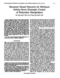
FIG. 2. The Ikeda map. Five hundred points of the Ikeda map are shown, both in original coordinates (x t ,y t ) 共upper panel兲 and reconstructed coordinates (x t ,x t⫹1 ) 共lower panel兲. Reconstruction of this map 共lower panel兲 is considerably less trivial than the equivalent reconstruction for either the logistic or He´non maps. 1. The Ikeda map

The simplest test we apply is reconstruction of the Ikeda map with the addition of various levels of dynamic noise. By dynamic noise we mean that system noise is added to the dynamics prior to prediction of the succeeding state. The Ikeda equations are given by x t⫹1 ⫽1⫹ ␮ 共 x t cos ␪ t ⫺y t sin ␪ t 兲 , y t⫹1 ⫽1⫹ ␮ 共 x t sin ␪ t ⫹y t cos ␪ t 兲 ,

␪ t ⫽0.4⫺

6 1⫹x 2t ⫹y 2t

.

The bifurcation parameter ␮ ⫽0.7 provides chaotic dynamics. We choose to examine this map because the reconstructed dynamics are much more complex than those of either the logistic map or the He´non map. Figure 2 shows 500 points of this map both in original and reconstructed coordinates. For trajectories of length 500, in the absence of noise, the modeling algorithm was able to accurately reproduce the delay reconstructed attractor.

FIG. 3. Reconstruction Ikeda map from a noisy trajectory. The noisy model data 共top panel兲 and the iterated noise free prediction from a model of these data 共lower panel, solid dots兲 are shown. The model generated dynamic behavior exactly equivalent to the original data. Even in the absence of noise the attractor produced from the model prediction is as ‘‘noisy’’ as that from the noisy data. The expected noise free dynamics are shown in Fig. 2. Comparing insample and out-sample predictions, this model appears to overfit the data. A second model which does not overfit the data 共in-sample and out-sample MSE: 1.25⫻10⫺3 and 2.15⫻10⫺3 ) produced a high order periodic orbit 共lower panel, open circles兲. The two models contained 91 and 25 nonlinear ‘‘neurons,’’ respectively. Correlation dimension estimates for the overfit model were equivalent to the data; for the smaller model these estimates are shown in Table I.

In virtually all real systems deterministic dynamics are corrupted by some dynamic noise 共noise that is intrinsic to the dynamics rather than added afterwards兲. We therefore repeat the Ikeda simulation with the addition of Gaussian random variates to each scalar component at each iteration. The standard deviation of the variates are set at 10% of the the standard deviation of the data. For this level of noise Fig. 3 shows the attractor reconstructed from the original data and attractors reconstructed from noiseless model simulations of length 500. One can see that from this short and noise section of data the basic features of the attractor have been extracted. Table I reveals that the noise free trajectory is a stable limit cycle. However, the limit cycle does lie on the true attractor 共Fig. 3兲. Furthermore, the addition of dynamic

066701-6

PHYSICAL REVIEW E 66, 066701 共2002兲

MINIMUM DESCRIPTION LENGTH NEURAL NETWORKS . . .

chaotic system are reproduced from the model of this short and noisy time series segment. Table I confirms that the correlation dimension estimates for the data and surrogates were comparable. Underestimation of correlation dimension for this data 共and possibly the experimental systems in the next section兲 is due to the finite short and noisy time series. Larger, noise free data produced more accurate estimates. Irrespective of this, the importance of Table I is as a comparison of statistic values 关5兴. With higher noise levels or shorter time series we found that the reconstructed dynamics did not satisfactorily mimic the true behavior. For longer or less noisy data segments we found that performance improved. B. Experimental data

We now present the application of this algorithm to data from three experimental systems: the Wolf annual sunspot time series 关25兴, experimental recordings of infant respiration 关26兴, and the chaotic laser data utilized in the 1992 Santa Fe time series competition 关11,27兴. We have deliberately selected these three sources of data because each of them has been the focus of considerable attempts to model the dynamics. FIG. 4. Reconstruction Ro¨ssler system from a noisy trajectory. The noisy model data 共top panel兲 and the iterated noisy free prediction from a model of these data 共bottom panel solid dots兲 are shown. Also shown in the bottom panel is a comparable noise free simulation of this system 共open circles兲. The model generated dynamic behavior equivalent to the differential equations in the absence of noise 共Table I兲. In-sample and out-sample MSE 共0.101 and 0.250兲 were comparable.

noise produces trajectories very similar to the original data. With models built from larger data sets, or lower noise levels the quality of the simulations improves and one obtains the expected chaotic dynamics.

1. Sunspots

The annual sunspot count time series has been the subject of substantial interest in both the physics and statistics communities. Tong 关26兴 describes models of this time series using both autoregressive 共AR兲 and self-exciting threshold autoregressive 共SETAR兲 models. Judd and Mees have subsequently shown that superior predictive performance can be achieved with nonlinear radial basis function models 关2,31兴. For fairness of comparison we transform the raw data according to y t 哫2 冑y t ⫹1⫺1.

2. The Ro¨ssler system

The second computational simulation we wish to consider is a chaotic flow. The Ro¨ssler system is given by x˙ ⫽⫺y⫺z, y˙ ⫽x⫹ay, z˙ ⫽b⫹z 共 x⫺c 兲 . For a⫽0.398, b⫽2, and c⫽4 the system exhibits ‘‘singleband’’ chaos. We integrated these equations with step size 0.5 adding dynamic noise to each component at each step 共and then using the noisy coordinates for the integration to the next time step兲 to generate 500 points of the system. From this noisy data we constructed a neural network model 共the optimal model had only 12 ‘‘neurons’’兲 using the methods described in Sec. III. Figure 4 shows the original embedded data, the reconstruction from a noise free simulation of the model and the clean attractor 共computed in the absence of noise兲. One can clearly see that the main features of this

共8兲

This transformation was selected by Tong to improve the performance of linear models with this highly non-Gaussian distributed data. Table II compares the mean sum of square prediction error achieved with our algorithm and the methods proposed by Tong 关26兴 and Judd and Mees 关2兴. Our main interest is not in the MSE, but in dynamic performance. Linear models described by Tong 关26兴 behave as a stable focus. The nonlinear methods described by Judd and Mees produce either stable foci 关2兴 or a stable periodic orbit 关31兴. Figure 5 shows that the algorithm described here generates chaotic dynamics that closely resemble the original time series. In Table I we observed fractional correlation dimension in both the data and model simulations. Furthermore, prediction over a longer time horizon shows that the methods described here perform better than the alternatives. The iterated model prediction shown in Fig. 5 exhibits dynamics remarkably similar to those observed in the historical data. By comparison, linear models clearly cannot capture the long term 共nonlinear兲 dynamics. Radial basis models described in 关2,31兴 exhibit stable periodic orbits and only

066701-7

PHYSICAL REVIEW E 66, 066701 共2002兲

M. SMALL AND C. K. TSE TABLE II. Mean free run prediction error for the annual sunspot count time series. Mean sum of the square of the prediction error for models of the sunspot time series produced with five different modeling techniques are reported. Values marked with * are those reported in 关2兴; † denotes a typical result from an equivalent model employing the methods described by 关2兴 共we do not have access to the earlier model兲. All other results are computed directly. Following Tong 关26兴, the AR共9兲 and reduced AR 共RAR兲 models are computed from the untransformed data. Applying the transformation 共8兲 produced similar results. The SETAR model is described in 关30兴. MSE Model AR共9兲 SETAR RAR Radial basis Neural network

1980–1988

1980–2002

334* 413* 214* 306* 625

416 1728 291 489† 356

approximate the true dynamics when driven by high dimensional noise. Although the predictions of Fig. 5 are qualitatively plausible, we do not claim them to be quantitatively accurate. Table II clearly shows that the neural network model behaves poorly for short term prediction. We are certainly not claiming to predict the observed values for the entire first half of this century. 2. Infant respiration

Radial basis models built with minimum description length have previously been tested with infant respiratory data 关4兴. These data are recordings of instantaneous abdominal cross section of human infants during normal sleep. It has

been shown that these data are not consistent with a linear noise process 关25兴 and that the data are consistent with the hypothesis of deterministic chaos. However, nonlinear radial basis models of these data typically behave as a noise driven periodic orbit 关4兴. While this result is consistent with the conclusions of 关25兴, it is perhaps unsatisfactory that the only deterministic structure that one may extract from these data is a periodic motion. It has recently been observed that in certain circumstances complex period doubling phenomenon may be used to describe this data 关32兴. This is an attractive observation, but the phenomenon has not been observed consistently in all such data using the methods described in 关32兴. In this section we apply the modeling algorithm described in this paper to several recordings of infant respiration. In each case we find that the MDL best model of this data exhibits chaotic dynamics and the free run behavior of the model behaves qualitatively similar to the data. Figure 6 depicts a representative data set and simulation. In Table I we see that correlation dimension for noisy simulations are comparable to the data 共but not without noise兲. Perhaps this is further evidence of the stochastic behavior left unmodeled by our algorithms 共a similar observation was made in 关25兴兲. 3. Chaotic laser dynamics

Our final test system is data from a chaotic laser experiment. This data was utilized in the 1992 Santa Fe time series competition. From a large number of potential modeling regimes a nearest neighbor technique 关27兴 and a neural network model were found to perform best 关12兴. We utilize the same data as described in 关12,27兴 to build a model using the algorithm described in Sec. III. Initial model results were relatively poor. We found that transforming the data so that it was normally distributed prior to modeling

FIG. 5. The annual sunspot count. The actual sunspot count and iterated predictions from a neural network model of these data 共the model is described in Table I兲. The top panel shows the actual sunspot count for each year of the period 1920–2000. The bottom panel shows a noiseless freerun 共iterated兲 prediction for the model of these data over a period of 80 years 共1980–2060兲. Actual known values are also shown 共circles兲 for the years 1980–2000. The free run prediction does not fit the dynamics exactly, but it does provide a good model of the dynamics. Qualitative features are common to both panels. The annual sunspot count is a dimensionless quantity derived from the number of sunspots observed throughout that year 共see 关26兴兲.

066701-8

PHYSICAL REVIEW E 66, 066701 共2002兲

MINIMUM DESCRIPTION LENGTH NEURAL NETWORKS . . .

FIG. 6. Human infant respiration. The top panel shows the short term prediction from infant respiration data. True data are depicted as circles; the model prediction is a solid line. The second and third panels show longer representative segments of both the original data 共second panel兲 and the MDL-best neural network model 共Table I兲 free-run prediction. The model is built from the data shown in the second panel and the free-run prediction is generated without any additional noise. In this example the model simulation does not exhibit the peak variation present in the data. All other features are comparable: the same irregular asymmetric wave form and frequent variation in amplitude are present in both the data and simulation, and both had correlation dimension exceeding 2. The measured abdominal area is proportional to the cross sectional area, but the units of measurement are arbitrary and have been rescaled to have a mean of zero and a standard deviation of one 关25兴.

produced far superior results. We believe that this data is sufficiently non-Gaussian so that the assumption that ␰ (x) ⫽x in Eq. 共7兲 is inappropriate. We are forced to impose an arbitrary transformation to aid the modeling algorithm and improve results. In Table III we quantitatively compare our prediction results to those presented in 关12,27兴. Figure 7 depicts representative results of the modeling algorithm with the inclusion of this static nonlinear transformation of the data. We note that the qualitative behavior of this model is comparable to the best modeling results of TABLE III. Mean free run prediction error for the chaotic laser data. NMSE for models of the laser time series produced with three different modeling techniques are reported. NMSE are computed for 100 point free run predictions initiated at datum number 1000, 2180, 3870, 4000, and 5180 共these initial conditions are those selected in 关27兴兲. Values marked with * are those reported in 关27兴.

Model

NMSE 1000

2180

3870

4000

5180

Sauer 关27兴 0.027* 0.065* 0.487* 0.023* 0.160* Wan 关12兴 0.077* 0.174* 0.183* 0.006* 0.111* MDL-neural network 0.066 0.061 0.086 0.479 0.038

Sauer 关27兴 and Wan 关12兴. Sauer’s model utilized a nearest neighbor technique 关27兴 and therefore does not provide an actual estimate of the equations of motion 共one cannot differentiate a nearest neighbor prediction兲. In 关12兴 user intervention is required to produce a plausible prediction. The dynamic behavior depicted in Fig. 7 is produced directly from the data. The NMSE of our modeling algorithm is not substantially better than those of 关12,27兴, but the qualitative behavior is better and the algorithm therefore provides equations of motion that are a more plausible model for the underlying dynamics. Table I confirms that the behavior of data and model simulations 共with and without noise兲 are remarkably similar. Perhaps indicating that this system 共unlike that in the previous section兲 is completely 共or largely兲 deterministic. The model prediction in Fig. 7 is typical of our results. But, we observed that small changes in the initial conditions of a model 共less than 0.01% of the data values兲 greatly changed the NMSE prediction error over the next 100 data. Using the expected values we were able to optimize the initial condition of the model and obtained improved ‘‘predictions.’’ Of course, these are not true predictions as they require knowledge of the actual trajectory. Rather, we are providing a maximum likelihood estimate 共MLE兲 of the ini-

066701-9

PHYSICAL REVIEW E 66, 066701 共2002兲

M. SMALL AND C. K. TSE

FIG. 7. Chaotic laser dynamics. Free-run prediction 共solid line兲 and actual data 共circles兲 for a MDL-best model of the chaotic laser data. The prediction error is shown as a dotted line 共NMSE of 0.0955兲. The simulated performance is qualitatively comparable to those presented in 关12兴. However, the neural network model described in 关12兴 ‘‘breaks down’’ soon after the collapse of the laser. We found that the neural network model was large and highly chaotic; tiny changes in the initial conditions yielded substantial variation in the model predictions. This model evidently exhibits extremely sensitive dependence on initial conditions and the uncertainty of this simulation as a prediction is therefore great. The laser intensity takes values from 0 to 255 共i.e., the units of measurement are arbitrary兲.

tial state given the observed trajectory. For that MLE value we compute a model simulation, the deviation between the actual observed value and the MLE of the initial state is substantially less than the coarse grain digitization of the model. Therefore, initial states that are indistinguishable to the experimental apparatus exhibit wildly varying performance. Such variation in prediction draws into doubt the significance of the relative small quantitative difference observed in the NMSE depicted in Table III. We prefer only to conclude that the model produced by this algorithm provided quantitatively realistic simulations, which for the correct choice of initial condition could shadow the true trajectory. V. CONCLUSION

Neural networks have a happy history of producing good 共and sometimes not so good兲 results in situations where the number of parameters exceeds the number of available data 共关12兴 provides a good example of both cases兲. However, this is not a contradiction of the statistical view that N data points may only be used to fit 共at most兲 N parameters. The important consideration is the precision with which one chooses to specify each parameter. Assuming infinite precision of every observation and parameter, a 共linear, linearly independent兲 problem with N observations is overdetermined if the number of parameters k is less than N. Conversely if k⭓N the problem is underdetermined and one can achieve an arbitrary fit to the data. By terminating the training of a network before optimization one obtains parameters with a relatively low precision and one is therefore able to specify a large number of them k⬎N. However, because parameter optimization is a nonlinear problem this premature termination leads to a local minima—very often repeated application will yield a different local minima and different model behavior. One then simply chooses the model that performs best on the training data. In an attempt to address this problem, predictive MDL 关15,16兴 and other information theoretic model selection criteria 关13兴 have been suggested in the literature. However, none of these techniques consider the precision with which

parameters must be specified. Because the MDL criterion described here computes the precision of the parameters one has a much fairer estimate of the best model of a particular data set. Furthermore, this avoids the need to waste 共often rare or valuable兲 data during cross validation 关10兴. We cannot prove that this algorithm will work best for any given data set. For any particular data set we actually expect this algorithm to be sub-optimal. However, theory shows that the functional form 共7兲 is adequate for any nonlinearity and, with sufficiently large d and k, it will capture the dynamics of a sufficiently long time series. Assuming the time series is sufficiently long 共let N 0 be the minimum such length, so that N⬎N 0 is sufficient兲, then there exists d 0 and k 0 such that the neural network 共7兲 captures the required nonlinearity. We rely on heuristic techniques to determine d 0 and MDL selection criteria is used to find k 0 . If N⬍N 0 then we have insufficient data to find the optimal model with this approach. In some situations other modeling algorithms may perform better: for example, a global polynomial model may model polynomial nonlinearities well. However, for N⬍N 0 MDL selection will still find the best model size k(d,N) given the available data. To justify our failure to find the optimal model in every case, we note that the combinatorial nature of this problem means that there is no known polynomial time algorithm to find a solution. One need only note that a restricted version of our MDL nonlinear model selection problem can be recast as the knapsack problem 关33兴. We therefore conclude that it is highly unlikely that an efficient generic algorithm exists for estimating the best neural network 共or basis function兲 model of a given data set. It is interesting to note that many of the modeling results presented here 共most notably those of the chaotic laser dynamics兲 exhibit the 共expected兲 sensitive dependence on initial conditions. This sensitivity is sufficient to generate a wide variety of dynamic evolution within the experimental precision of the raw data. The data are digitized as 10-bit integers. However, change in initial condition of less than 0.001 共in each component兲 provided indistinguishable initial conditions but NMSE over the prediction range of 100 val-

066701-10

PHYSICAL REVIEW E 66, 066701 共2002兲

MINIMUM DESCRIPTION LENGTH NEURAL NETWORKS . . .

ues varies between the optimal results shown in Table III and NMSE greater than 1. Therefore, if this model is an accurate representation of the dynamics in question, then comparing NMSE over this horizon is irrelevant because of the excessive uncertainty in the initial conditions. One should test how well the model captures the dynamics. NMSE 共either one step or iterates as in Tables II and III兲 is a poor measure of dynamic fit. The correlation dimension or other dynamic invariants are far better 共see Table I兲 关5兴. We do not emphasize the predictive power of this algorithm. Each of the systems tested was potentially chaotic. We demonstrated for the laser data that prediction from the model was poor because of the sensitive dependence on initial conditions and possible undersampling of the original experiment. However, in each of the experimental systems we found that the qualitative behavior of model simulations was highly accurate. Realistic chaotic dynamics were observed for the sunspot time series. Simulations of infant respirations appear indistinguishable from real data. Finally, simulations from models of the Santa Fe laser data exhibited the same features as the data and achieved 共for optimal selection of initial conditions兲 free-run prediction that exceeded previous results. Comparing dynamic invariants of the data and model simulations showed good agreement

共Table I兲 and provided a fairer and more useful test of ‘‘goodness’’ of the models. Finally, we note that model prediction errors of test and fit data observed for the simulated systems were not exactly equal. We have observed, for MDL-best models a slight, but systematic overfitting of the data. The one-step in-sample MSE values quoted in Figs. 3 and 4 were systematically lower than the corresponding out-sample MSE. This is due to a flaw in the current algorithm. To alleviate computational burden we assumed that the only significant parameters ⌳ k were the linear ones (␭ 0 ,␭ 1 , . . . ,␭ k ). While this is clearly only an approximation it seems to produce adequate results. For the case of radial basis models it was found that the additional expense of computing the full description length provided only a slight advantage for the final model 关4兴. It is likely that the improvement in neural network models afforded by the full calculation would also be marginal.

关1兴 J. Rissanen, Stochastic Complexity in Statistical Inquiry 共World Scientific, Singapore, 1989兲. 关2兴 K. Judd and A. Mees, Physica D 82, 426 共1995兲. 关3兴 A pseudolinear nonlinear model is a model that is a nonlinear function of the model variables, but only a linear function of the model parameters 关18兴. 关4兴 M. Small and K. Judd, Physica D 117, 283 共1998兲. 关5兴 M. Small and K. Judd, Physica D 120, 386 共1998兲. 关6兴 M. Small, D. Yu, R. Clayton, T. Eftesto” l, and R. G. Harrison, Int. J. Bifurcation Chaos Appl. Sci. Eng. 11, 2531 共2001兲. 关7兴 R. Brown, N. F. Rulkov, and E. R. Tracy, Phys. Lett. A 194, 71 共1994兲. 关8兴 M. Small, K. Judd, and A. Mees, Phys. Rev. E 65, 046704 共2002兲. 关9兴 A. Leonardis and H. Bischof, Neural Networks 11, 963 共1998兲. 关10兴 H. Leung, T. Lo, and S. Wang, IEEE Trans. Neural Netw. 12, 1163 共2001兲. 关11兴 N. Gershenfeld, The Nature of Mathematical Modeling 共Cambridge University Press, Cambridge, England, 1999兲. 关12兴 E. A. Wan, in Time Series Prediction: Forecasting the Future and Understanding the Past, Vol. XV of Studies in the Sciences of Complexity, edited by A. Weigend and N. Gershenfeld, Santa Fe Institute, 共Addison-Wesley, Reading, MA, 1993兲, pp. 195–217. 关13兴 D. B. Fogel, IEEE Trans. Neural Netw. 2, 490 共1991兲. 关14兴 H. Akaike, IEEE Trans. Autom. Control 19, 716 共1974兲. 关15兴 M. Lehtokangas, J. Saarinen, and K. Kaski, Appl. Math. Comput. 75, 151 共1996兲. 关16兴 M. Lehtokangas, J. Saarinen, P. Huuhtanen, and K. Kaski, Neural Comput. 8, 583 共1996兲. 关17兴 G. Schwarz, Ann. Stat. 6, 461 共1978兲.

关18兴 W. H. Press, B. P. Flannery, S. A. Teukolsky, and W. T. Vetterling, Numerical Recipes in C 共Cambridge University Press, Cambridge, England, 1988兲. 关19兴 D. Rumelhart, R. Durbin, R. Golden, and Y. Chauvin, in Mathematical Perspectives on Neural Networks, edited by P. Smolensky, P. Mozer, M. Rumelhart, and D. Rumelhart 共Lawrence Erlbaum Associates, Hillsdale, NJ, 1996兲, pp. 533–566. 关20兴 Because the model is a linear combination of linearly independent functions, this is obvious. 关21兴 Cross validation is a model selection criteria. The available data is divided into two sections: fit data and test data. The model is then fitted to the fit data and the model selection determined by the performance on the test data. Of course, the test data must be known prior to modeling, and is part of the model building process 共one cannot use it for ‘‘honest’’ test predictions兲. 关22兴 Description length D(k) will depend on the particular time series under consideration and the model selected. Computation of M (k) and E(k) will depend on the particular encoding once chooses for the model and for rational numbers. We use the optimal encoding of floating point numbers described by Rissanen 关1兴. 关23兴 D. P. Mandic and J. A. Chambers, Recurrent Neural Networks for Prediction 共Wiley, London, 2001兲. 关24兴 S. Ellacott and D. Bose, Neural Networks: Deterministic Methods of Analysis 共Thomson Computer Press, London, 1996兲. 关25兴 M. Small, K. Judd, M. Lowe, and S. Stick, J. Appl. Physiol. 86, 359 共1999兲. 关26兴 H. Tong, Non-linear Time Series: A Dynamical Systems Approach 共Oxford University Press, New York, 1990兲. 关27兴 T. Sauer, in Time Series Prediction: Forecasting the Future

ACKNOWLEDGMENTS

This work was supported by a Hong Kong Polytechnic University research grant 共No. G-YW55兲. The authors acknowledge the helpful comments of Z. Yang and J. P. Barnard regarding neural network technology.

066701-11

PHYSICAL REVIEW E 66, 066701 共2002兲

M. SMALL AND C. K. TSE and Understanding the Past, 共Ref. 关12兴兲, pp. 175–193. 关28兴 D. Yu, M. Small, R.G. Harrison, and C. Diks, Phys. Rev. E 61, 3750 共2000兲. 关29兴 The hypothesis is that the model adequately described the dynamics. 关30兴 D. Ghaddar and H. Tong, Appl. Stat. 30, 238 共1981兲. 关31兴 K. Judd and A. Mees, Physica D 120, 273 共1998兲. 关32兴 M. Small, D. Yu, and R. G. Harrison, in Space Time Chaos: Characterization, Control and Synchronization, edited by S.

Boccaletti, J. Burguete, W. G. -V. nas, H. Mancini, and D. Valladares 共World Scientific, Singapore, 2001兲, pp. 3–18. 关33兴 The knapsack problem is a known NP-complete problem. If a given problem can be recast as an NP complete problem then it too is NP-complete. All NP-complete problems are equivalent and are as computationally difficult as 共for example兲 the traveling salesman problem. Therefore, the problem we consider here has no 共known兲 polynomial time solution.

066701-12