The McCabe-Thiele diagram where y is plotted as a function x along the column .... Figure 2.8: McCabe-Thiele diagram for the same example as in Figure 2.7: ...
Minimum Energy Requirements in Complex Distillation Arrangements by Ivar J. Halvorsen
A thesis submitted for the degree of Dr.Ing.
May 2001 Department of Chemical Engineering Norwegian University of Science and Technology N-7491 Trondheim, Norway Dr. ing. Thesis 2001:43 ISBN 82-471-5304-1 ISSN 0809-103X
NTNU Dr. ing. Thesis 2001:43
Ivar J. Halvorsen
2
NTNU Dr. ing. Thesis 2001:43
Ivar J. Halvorsen
Preface The Norwegian Dr.Ing (Ph.D) degree requires a basic research work and approximately one full year of courses at graduate and postgraduate level. This report presents the main scientific results from the research. However, there are also interesting issues on how the results were obtained, which are not covered. Some of these issues are the work progress, development and use of computational tools like numerical methods for optimization, nonlinear equation solving, simulation and control, and the software itself. In all basic research, the results themselves cannot be planned for, only the activities which may or may not lead up to new results. In this process, we sometimes discover new interesting directions. This applies for the results presented in chapters 3-6. The research started out in the direction of optimizing control, but it was discovered that we were able to find some new basic relationships in a system of integrated distillation columns, and that thread was followed in more detail. My background is from the department of Engineering Cybernetics, NTNU, where I graduated in 1982, and for me it have also been interesting to take the step into Chemical Engineering. There are some obvious cultural differences in how to approach an engineering task. I think it can be summed up in that the chemical engineer focuses more on the design of a process, while the control engineer focuses more on its operation. Clearly, a combination of these approaches is needed. In control engineering, we must look more into the process and influence the design to get more controllable units and plants. It also helps the control engineer to have a basic understanding of the process behaviour. In process design, chemical engineers should put more attention to the dynamic properties and control technology and use this knowledge to design more compact processes with better overall performance. I feel that in particular for complex integrated processes, combined focus on process design and operation is vital since the potential benefit of the integration can easily be lost if the process is not properly controlled.
NTNU Dr. ing. Thesis 2001:43
Ivar J. Halvorsen
4 I have some years of experience from industry and as a research scientist at SINTEF, the research foundation at NTNU. Unlike the work at SINTEF, where an industrial customer usually is directly awaiting the results from a project, the customer for the Dr.Ing. has several faces. There is a financial sponsor, a supervisor, the candidate himself and the international community of researchers in the field. It is clear that the most demanding “customer” has to be the candidate himself in order to obtain the best results. I have had numerous fruitful discussions with my supervisor, professor Sigurd Skogestad at the Chemical Engineering Department. He has been a continuous source of inspiration, and has provided invaluable contributions both in the research work and to help me focus on the reader during writing of this thesis. In Skogestad’s process control group Atle C. Christiansen and John Morud gave important inputs on integrated column arrangements, and I will also mention Bernd Wittgens, Truls Larsson, Audun Faanes, Eva-Katrine Hilmen, Tore Lid, Marius Govatsmark, Stathis Skouras and the latest arrivals Espen Storkaas and Vidar Alstad. I thank Hilde Engelien for reading the manuscript and giving valuable feedback. I shared an office with Edvard Sivertsen, who studied membrane separation, and we discussed everything from thermodynamics to raising children. I hope he forgives me for all the lecturing about distillation every time I felt that I had discovered something. I am also grateful for discussions with the visiting professors Valeri Kiva (1996/97) and David Clough (1999/2000). We also had the opportunity to meet Felix Petlyuk who visited Trondheim in May 1997. As an introduction to Petlyuk arrangements, NTNU participated in a European research project within the Joule 3 programme: DISC, Complex distillation columns. One spin-off was the visit by Maria Serra in june 1998, resulting in the paper in Chapter 11. I also thank my employer SINTEF for support, in addition to the grant from the Norwegian Research Council through the REPP programme. Finally I thank my wife Toril, and my children Øyvind, Berit and Maria for giving me a wider perspective on things. The work has consumed a lot of time and attention for some years now and Berit, who is 10 years old, asked me: “How many theses have you written now? Only one?”
NTNU Dr. ing. Thesis 2001:43
Ivar J. Halvorsen
Summary Distillation is the most widely used industrial separation technology and distillation units are responsible for a significant part of the total heat consumption in the world’s process industry. In this work we focus on directly (fully thermally) coupled column arrangements for separation of multicomponent mixtures. These systems are also denoted Petlyuk arrangements, where a particular implementation is the dividing wall column. Energy savings in the range of 20-40% have been reported with ternary feed mixtures. In addition to energy savings, such integrated units have also a potential for reduced capital cost, making them extra attractive. However, the industrial use has been limited, and difficulties in design and control have been reported as the main reasons. Minimum energy results have only been available for ternary feed mixtures and sharp product splits. This motivates further research in this area, and this thesis will hopefully give some contributions to better understanding of complex column systems. In the first part we derive the general analytic solution for minimum energy consumption in directly coupled columns for a multicomponent feed and any number of products. To our knowledge, this is a new contribution in the field. The basic assumptions are constant relative volatility, constant pressure and constant molar flows and the derivation is based on Underwood’s classical methods. An important conclusion is that the minimum energy consumption in a complex directly integrated multi-product arrangement is the same as for the most difficult split between any pair of the specified products when we consider the performance of a conventional two-product column. We also present the Vmin-diagram, which is a simple graphical tool for visualisation of minimum energy related to feed distribution. The Vmin-diagram provides a simple mean to assess the detailed flow requirements for all parts of a complex directly coupled arrangement. The main purpose in the first part of the thesis has been to present a complete theory of minimum energy in directly coupled columns, not a design procedure for engineering purposes. Thus, our focus has been on the basic theory and on verification and analysis of the new results. However, based on these results, it is
NTNU Dr. ing. Thesis 2001:43
Ivar J. Halvorsen
6 straightforward to develop design procedures including rigorous computations for real feed mixtures without the idealized assumptions used to deduce the analytic results. In part 2 we focus on optimization of operation, and in particular the concept of self-optimizing control. We consider a process where we have more degrees of freedom than are consumed by the product specifications. The remaining unconstrained degrees of freedom are used to optimize the operation, given by some scalar cost criterion. In addition there will in practice always be unknown disturbances, model uncertainty and uncertainty in measurements and implementation of manipulated inputs, which makes it impossible to precalculate and implement the optimal control inputs accurately. The main idea is to achieve self-optimizing control by turning the optimization problem into a constant setpoint problem. The issue is then to find (if possible) a set of variables, which when kept at their setpoints, indirectly ensures optimal operation. We have used the ternary Petlyuk arrangement to illustrate the concept. It is a quite challenging case where the potential energy savings may easily be lost if we do not manage to keep the manipulated inputs at their optimal values, and the optimum is strongly affected by changes in feed composition and column performance. This also applies to the best control structure selection, and we believe that the reported difficulties in control are really a control structure problem (the task of selecting the best variables to control and the best variables to manipulate). In this analysis we present in detail the properties of the Petlyuk arrangement, and show how important characteristics depend on the feed properties and product purity. We have used finite stage-by-stage models, and we also show how to use Underwood’s equations to compute the energy consumption for infinite number of stages for any values of the degrees of freedom. Such computations are very simple. The results are accurate and in terms of computation time, outperform simulations with finite stage-by-stage models by several magnitudes. The analysis gives a basic understanding of the column behaviour and we may select operating strategies based on this knowledge for any given separation case. In some cases there will be a quite flat optimality region, and this suggests that one of the manipulated inputs may be kept constant. We also show that the side-stream purity has strong impact on the optimality region. One observation is that a symptom of sub-optimal operation can be that we are unable to achieve high sidestream purity, and not necessarily increased energy consumption. In summary, the presented results contribute to improved understanding and removal of some uncertainties in the design and operation of directly integrated distillation arrangements.
NTNU Dr. ing. Thesis 2001:43
Ivar J. Halvorsen
7 Preface
3
Summary
5
Notation and Nomenclature
19
1 Introduction
21
1.1 Rationale . . . . . . . . . . . . . . . . . . . . . . . . . . . . . . . . . . . . . . . . . . . . . . . 21 1.2 Contributions of the Thesis . . . . . . . . . . . . . . . . . . . . . . . . . . . . . . . . . 22 1.3 Thesis Outline . . . . . . . . . . . . . . . . . . . . . . . . . . . . . . . . . . . . . . . . . . . 23 1.3.1
Part I: Design . . . . . . . . . . . . . . . . . . . . . . . . . . . . . . . . . . . . . 23
1.3.2
Part II: Operation . . . . . . . . . . . . . . . . . . . . . . . . . . . . . . . . . . 24
Part I: Design
25
2 Distillation Theory
27
2.1 Introduction . . . . . . . . . . . . . . . . . . . . . . . . . . . . . . . . . . . . . . . . . . . . . 28 2.2 Fundamentals . . . . . . . . . . . . . . . . . . . . . . . . . . . . . . . . . . . . . . . . . . . . 29 2.2.1
The Equilibrium Stage Concept . . . . . . . . . . . . . . . . . . . . . . . 29
2.2.2
Vapour-Liquid Equilibrium (VLE) . . . . . . . . . . . . . . . . . . . . 29
2.2.3
K-values and Relative Volatility . . . . . . . . . . . . . . . . . . . . . . 31
2.2.4
Estimating the Relative Volatility From Boiling Point Data . 32
2.2.5
Material Balance on a Distillation Stage . . . . . . . . . . . . . . . . 34
2.2.6
Assumption about Constant Molar Flows . . . . . . . . . . . . . . . 36
2.3 The Continuous Distillation Column . . . . . . . . . . . . . . . . . . . . . . . . . . 36 2.3.1
Degrees of Freedom in Operation of a Distillation Column . 37
2.3.2
External and Internal Flows . . . . . . . . . . . . . . . . . . . . . . . . . . 38
2.3.3
McCabe-Thiele Diagram . . . . . . . . . . . . . . . . . . . . . . . . . . . . 38
2.3.4
Typical Column Profiles — Not optimal feed location . . . . . 40
2.4 Simple Design Equations . . . . . . . . . . . . . . . . . . . . . . . . . . . . . . . . . . . 41 2.4.1
Minimum Number of Stages — Infinite Energy . . . . . . . . . . 41
2.4.2
Minimum Energy Usage — Infinite Number of Stages . . . . . 42
2.4.3
Finite Number of Stages and Finite Reflux . . . . . . . . . . . . . . 43
2.4.4
Constant K-values — Kremser Formulas . . . . . . . . . . . . . . . 44
NTNU Dr. ing. Thesis 2001:43
Ivar J. Halvorsen
8 2.4.5
Approximate Formula with Constant Relative Volatility . . . 45
2.4.6
Optimal Feed Location . . . . . . . . . . . . . . . . . . . . . . . . . . . . . 47
2.4.7
Summary for Continuous Binary Columns . . . . . . . . . . . . . . 48
2.5 Multicomponent Distillation — Underwood’s Method . . . . . . . . . . . 51 2.5.1
The Basic Underwood Equations . . . . . . . . . . . . . . . . . . . . . 51
2.5.2
Stage to Stage Calculations . . . . . . . . . . . . . . . . . . . . . . . . . . 53
2.5.3
Some Properties of the Underwood Roots . . . . . . . . . . . . . . 54
2.5.4
Minimum Energy — Infinite Number of Stages . . . . . . . . . . 55
2.6 Further Discussion of Specific Issues . . . . . . . . . . . . . . . . . . . . . . . . . 58 2.6.1
The Energy Balance and Constant Molar Flows . . . . . . . . . . 58
2.6.2
Calculating Temperature when Using Relative Volatilities . 60
2.6.3
Discussion and Caution . . . . . . . . . . . . . . . . . . . . . . . . . . . . . 62
2.7 Bibliography . . . . . . . . . . . . . . . . . . . . . . . . . . . . . . . . . . . . . . . . . . . . 62 3 Analytic Expressions and Visualization of Minimum Energy Consumption in Multicomponent Distillation: A Revisit of the Underwood Equations.
63
3.1 Introduction . . . . . . . . . . . . . . . . . . . . . . . . . . . . . . . . . . . . . . . . . . . . . 64 3.1.1
Background . . . . . . . . . . . . . . . . . . . . . . . . . . . . . . . . . . . . . . 64
3.1.2
Problem Definition - Degrees of Freedom . . . . . . . . . . . . . . 65
3.2 The Underwood Equations for Minimum Energy . . . . . . . . . . . . . . . 65 3.2.1
Some Basic Definitions . . . . . . . . . . . . . . . . . . . . . . . . . . . . . 65
3.2.2
Definition of Underwood Roots . . . . . . . . . . . . . . . . . . . . . . 66
3.2.3
The Underwood Roots for Minimum Vapour Flow . . . . . . . 67
3.2.4
Computation Procedure . . . . . . . . . . . . . . . . . . . . . . . . . . . . . 68
3.2.5
Summary on Use of Underwood’s Equations . . . . . . . . . . . . 72
3.3 The Vmin-diagram (Minimum Energy Mountain) . . . . . . . . . . . . . . . 73 3.3.1
Feasible Flow Rates in Distillation . . . . . . . . . . . . . . . . . . . . 74
3.3.2
Computation Procedure for the Multicomponent Case . . . . . 75
3.3.3
Binary Case . . . . . . . . . . . . . . . . . . . . . . . . . . . . . . . . . . . . . . 75
3.3.4
Ternary Case . . . . . . . . . . . . . . . . . . . . . . . . . . . . . . . . . . . . . 78
NTNU Dr. ing. Thesis 2001:43
Ivar J. Halvorsen
9 3.3.5
Five Component Example . . . . . . . . . . . . . . . . . . . . . . . . . . . 81
3.3.6
Simple Expression for the Regions Under the Peaks . . . . . . . 82
3.4 Discussion . . . . . . . . . . . . . . . . . . . . . . . . . . . . . . . . . . . . . . . . . . . . . . 83 3.4.1
Specification of Recovery vs. Composition . . . . . . . . . . . . . . 83
3.4.2
Behaviour of the Underwood Roots . . . . . . . . . . . . . . . . . . . . 83
3.4.3
Composition Profiles and Pinch Zones . . . . . . . . . . . . . . . . . 85
3.4.4
Constant Pinch-zone Compositions (Ternary Case) . . . . . . . 85
3.4.5
Invariant Multicomponent Pinch-zone Compositions . . . . . . 89
3.4.6
Pinch Zones for V>Vmin . . . . . . . . . . . . . . . . . . . . . . . . . . . . 90
3.4.7
Finite Number of Stages . . . . . . . . . . . . . . . . . . . . . . . . . . . . . 90
3.4.8
Impurity Composition with Finite Number of Stages . . . . . . 92
3.5 Summary . . . . . . . . . . . . . . . . . . . . . . . . . . . . . . . . . . . . . . . . . . . . . . . 92 3.6 References . . . . . . . . . . . . . . . . . . . . . . . . . . . . . . . . . . . . . . . . . . . . . . 93 4 Minimum Energy for Three-product Petlyuk Arrangements
95
4.1 Introduction . . . . . . . . . . . . . . . . . . . . . . . . . . . . . . . . . . . . . . . . . . . . . 96 4.2 Background . . . . . . . . . . . . . . . . . . . . . . . . . . . . . . . . . . . . . . . . . . . . . 97 4.2.1
Brief Description of the Underwood Equations . . . . . . . . . . . 97
4.2.2
Relation to Previous Minimum Energy Results . . . . . . . . . . . 98
4.2.3
The Vmin-diagram for Conventional Columns . . . . . . . . . . . 99
4.3 The Underwood Equations Applied to Directly Coupled Sections . . 100 4.3.1
The Petlyuk Column Prefractionator . . . . . . . . . . . . . . . . . . 100
4.3.2
Composition Profiles . . . . . . . . . . . . . . . . . . . . . . . . . . . . . . 101
4.3.3
Reverse Net Flow of Components . . . . . . . . . . . . . . . . . . . . 102
4.3.4
Reverse Flow Effects on the Underwood Roots . . . . . . . . . 104
4.4 “Carry Over” Underwood Roots in Directly Coupled Columns . . . . 105 4.5 Vmin-Diagram for Directly Coupled Columns . . . . . . . . . . . . . . . . . 108 4.6 Minimum Energy of a Ternary Petlyuk Arrangement . . . . . . . . . . . . 110 4.6.1
Coupling Column C22 with Columns C21 and C1 . . . . . . . 110
4.6.2
Visualization in the Vmin-diagram . . . . . . . . . . . . . . . . . . . 112
NTNU Dr. ing. Thesis 2001:43
Ivar J. Halvorsen
10 4.6.3
Nonsharp Product Specifications . . . . . . . . . . . . . . . . . . . . 115
4.6.4
The Flat Optimality Region . . . . . . . . . . . . . . . . . . . . . . . . . 115
4.7 Improved 2nd Law Results in Petlyuk Arrangements . . . . . . . . . . . 117 4.8 Minimum Energy with Multicomponent Feed . . . . . . . . . . . . . . . . . 118 4.8.1
The General Rule . . . . . . . . . . . . . . . . . . . . . . . . . . . . . . . . . 119
4.8.2
Example: Sharp Component Splits in Products . . . . . . . . . 119
4.8.3
Example: Nonsharp Product Split . . . . . . . . . . . . . . . . . . . . 121
4.9 Discussion . . . . . . . . . . . . . . . . . . . . . . . . . . . . . . . . . . . . . . . . . . . . . 122 4.9.1
The Conventional Reference . . . . . . . . . . . . . . . . . . . . . . . . 122
4.9.2
Extra Condenser or Reboiler in the Prefractionator . . . . . . 123
4.9.3
Use of a Conventional Prefractionator Column . . . . . . . . . 125
4.9.4
Heat Integration . . . . . . . . . . . . . . . . . . . . . . . . . . . . . . . . . . 125
4.9.5
The Two-Shell Agrawal Arrangement . . . . . . . . . . . . . . . . 126
4.9.6
A Simple Stage Design Procedure . . . . . . . . . . . . . . . . . . . 126
4.9.7
Possible Reduction of Stages . . . . . . . . . . . . . . . . . . . . . . . 127
4.9.8
Short Note on Operation and Control . . . . . . . . . . . . . . . . . 129
4.10 Conclusion . . . . . . . . . . . . . . . . . . . . . . . . . . . . . . . . . . . . . . . . . . . . 130 4.11 References . . . . . . . . . . . . . . . . . . . . . . . . . . . . . . . . . . . . . . . . . . . . . 131 5 Minimum Energy for Separation of Multicomponent Mixtures in Directly Coupled Distillation Arrangements
135
5.1 Introduction . . . . . . . . . . . . . . . . . . . . . . . . . . . . . . . . . . . . . . . . . . . . 136 5.2 Four Components and Four Products . . . . . . . . . . . . . . . . . . . . . . . . 137 5.2.1
Extended Petlyuk Arrangement . . . . . . . . . . . . . . . . . . . . . . 137
5.2.2
Minimum Vapour Flow Expressions . . . . . . . . . . . . . . . . . 138
5.2.3
Visualization in the Vmin-Diagram . . . . . . . . . . . . . . . . . . 140
5.2.4
The Highest Peak Determines the Minimum Vapour Flow 142
5.2.5
Composition at the Junction C21-C22-C32 . . . . . . . . . . . . 143
5.2.6
Flows at the Feed Junction to C32 . . . . . . . . . . . . . . . . . . . 144
5.2.7
Composition Profile - Simulation Example . . . . . . . . . . . . 145
5.3 Minimum Energy for N Components and M Products . . . . . . . . . . . 146
NTNU Dr. ing. Thesis 2001:43
Ivar J. Halvorsen
11 5.3.1
Vmin for N Feed Components and N Pure Products . . . . . . 147
5.3.2
General Vmin for N Feed Components and M Products . . . 148
5.4 Verification of the Minimum Energy Solution . . . . . . . . . . . . . . . . . 150 5.4.1
Minimum Vapour Flow as an Optimization Problem . . . . . 151
5.4.2
Requirement for Feasibility . . . . . . . . . . . . . . . . . . . . . . . . . 151
5.4.3
Verification of The Optimal Solution . . . . . . . . . . . . . . . . . 152
5.4.4
Summary of the Verification . . . . . . . . . . . . . . . . . . . . . . . . 155
5.4.5
The Optimality Region . . . . . . . . . . . . . . . . . . . . . . . . . . . . . 156
5.5 Discussion . . . . . . . . . . . . . . . . . . . . . . . . . . . . . . . . . . . . . . . . . . . . . 157 5.5.1
Arrangement Without Internal Mixing . . . . . . . . . . . . . . . . 157
5.5.2
Practical Petlyuk Arrangements (4-product DWC). . . . . . . 159
5.5.3
Heat Exchangers at the Sidestream Junctions . . . . . . . . . . . 162
5.5.4
The Kaibel column or the “ column” . . . . . . . . . . . . . . . . . . 163
5.5.5
Required Number of Stages - Simple Design Rule . . . . . . . 163
5.5.6
Control . . . . . . . . . . . . . . . . . . . . . . . . . . . . . . . . . . . . . . . . . 164
5.6 Conclusion . . . . . . . . . . . . . . . . . . . . . . . . . . . . . . . . . . . . . . . . . . . . . 164 5.7 References . . . . . . . . . . . . . . . . . . . . . . . . . . . . . . . . . . . . . . . . . . . . . 165 6 Minimum Energy Consumption in Multicomponent Distillation
169
6.1 Introduction . . . . . . . . . . . . . . . . . . . . . . . . . . . . . . . . . . . . . . . . . . . . 170 6.1.1
Some Terms . . . . . . . . . . . . . . . . . . . . . . . . . . . . . . . . . . . . . 170
6.1.2
Basic Assumptions . . . . . . . . . . . . . . . . . . . . . . . . . . . . . . . . 171
6.1.3
Minimum Entropy Production (2nd law efficiency) . . . . . . 172
6.1.4
Minimum Energy (1st law) . . . . . . . . . . . . . . . . . . . . . . . . . 173
6.1.5
Summary of some Computation Examples . . . . . . . . . . . . . 174
6.2 The Best Adiabatic Arrangement Without Internal Heat Exchange . 176 6.2.1
Direct Coupling Gives Minimum Vapour Flow . . . . . . . . . 176
6.2.2
Implications for Side-Strippers and Side-Rectifiers . . . . . . . 179
6.2.3
The Adiabatic Petlyuk Arrangement is Optimal . . . . . . . . . 179
6.3 Entropy Production in Adiabatic Arrangements . . . . . . . . . . . . . . . . 180
NTNU Dr. ing. Thesis 2001:43
Ivar J. Halvorsen
12 6.3.1
Adiabatic Column (Section) . . . . . . . . . . . . . . . . . . . . . . . . 180
6.3.2
Adiabatic Petlyuk Arrangements . . . . . . . . . . . . . . . . . . . . . 181
6.4 Reversible Distillation . . . . . . . . . . . . . . . . . . . . . . . . . . . . . . . . . . . 182 6.4.1
The Reversible Petlyuk Arrangement . . . . . . . . . . . . . . . . . 183
6.4.2
Comparing Reversible and Adiabatic Arrangements . . . . . 187
6.5 A Case Study: Petlyuk Arrangements with Internal Heat Exchange . . . . . . . . . . . . . . . . . . . . . . . . . . . . . . . 188 6.5.1
Example 0: Theoretical Minimum Energy Limit . . . . . . . . 188
6.5.2
Example 1: Internal Heat Exchange in the Reversible Arrangement . . . . . . . . . . . . . 188
6.5.3
Example 2: Heat Exchange Across the Dividing Wall . . . . 189
6.5.4
Example 3: Pre-heating of the Feed by Heat Exchange with the Sidestream . . . . . . . . . 190
6.5.5
Summary of The Examples . . . . . . . . . . . . . . . . . . . . . . . . . 191
6.6 Operation at Several Pressure Levels . . . . . . . . . . . . . . . . . . . . . . . . 192 6.6.1
Example 1: Feed Split (Binary Case) . . . . . . . . . . . . . . . . . 192
6.6.2
Example 2: Double Effect Direct Split (DEDS) . . . . . . . . . 193
6.6.3
Example 3: Double Effect Prefractionator Column (DEPC) 194
6.6.4
Relation to the Petlyuk Column and the Vmin-diagram . . . 194
6.7 Discussion . . . . . . . . . . . . . . . . . . . . . . . . . . . . . . . . . . . . . . . . . . . . . 196 6.7.1
Plant-wide Issues . . . . . . . . . . . . . . . . . . . . . . . . . . . . . . . . . 196
6.7.2
Heat Exchange at the Sidestream Stages . . . . . . . . . . . . . . . 196
6.7.3
Non-Uniqueness of Heat Supply in Reversible Columns . . 197
6.7.4
Practical Issues . . . . . . . . . . . . . . . . . . . . . . . . . . . . . . . . . . 199
6.8 Conclusion . . . . . . . . . . . . . . . . . . . . . . . . . . . . . . . . . . . . . . . . . . . . 199 6.9 References . . . . . . . . . . . . . . . . . . . . . . . . . . . . . . . . . . . . . . . . . . . . . 200 6.10 Appendix: Reversible Distillation Theory . . . . . . . . . . . . . . . . . . . . 201 6.10.1 Temperature-Composition-Pressure Relationship . . . . . . . 202 6.10.2 The Reversible Vapour Flow Profile . . . . . . . . . . . . . . . . . . 203 6.10.3 Entropy Production in a Reversible Section . . . . . . . . . . . . 204 6.10.4 Reversible Binary Distillation . . . . . . . . . . . . . . . . . . . . . . . 205
NTNU Dr. ing. Thesis 2001:43
Ivar J. Halvorsen
13 Part II: Operation
209
7 Optimal Operation of Petlyuk Distillation: Steady-State Behaviour
211
7.1 Introduction . . . . . . . . . . . . . . . . . . . . . . . . . . . . . . . . . . . . . . . . . . . . 212 7.2 The Petlyuk Column Model . . . . . . . . . . . . . . . . . . . . . . . . . . . . . . . 215 7.3 Optimization Criterion . . . . . . . . . . . . . . . . . . . . . . . . . . . . . . . . . . . . 216 7.3.1
Criterion with State Space Model . . . . . . . . . . . . . . . . . . . . 217
7.4 Results From the Model Case Study . . . . . . . . . . . . . . . . . . . . . . . . . 218 7.4.1
Optimal Steady State Profiles . . . . . . . . . . . . . . . . . . . . . . . 218
7.4.2
The Solution Surface . . . . . . . . . . . . . . . . . . . . . . . . . . . . . . 220
7.4.3
Effect of Disturbances . . . . . . . . . . . . . . . . . . . . . . . . . . . . . 222
7.4.4
Transport of Components . . . . . . . . . . . . . . . . . . . . . . . . . . . 222
7.5 Analysis from Model with Infinite Number of Stages . . . . . . . . . . . 224 7.5.1
Minimum Energy Consumption for a Petlyuk Column. . . . 225
7.5.2
Solution Surface for Infinite Number of Stages . . . . . . . . . . 226
7.5.3
Analyzing the Effect of the Feed Enthalpy . . . . . . . . . . . . . 230
7.5.4
How Many Degrees of Freedom Must we Adjust During Operation? . . . . . . . . . . . . . . . . . . . . . . . . . . 230
7.5.5
Sensitivity to Disturbances and Model Parameters . . . . . . . 233
7.5.6
A Simple Control Strategy with one Degree of Freedom Fixed . . . . . . . . . . . . . . . . . . . . . . . . . . . . . . . . . . . 233
7.5.7
Liquid Fraction: Bad Disturbance or Extra Degree of Freedom? . . . . . . . . . . 234
7.5.8
Relations to Composition Profiles . . . . . . . . . . . . . . . . . . . . 234
7.6 Candidate Feedback Variables . . . . . . . . . . . . . . . . . . . . . . . . . . . . . 236 7.6.1
Position of Profile in Main Column (Y1). . . . . . . . . . . . . . . 236
7.6.2
Temperature Profile Symmetry (Y2) . . . . . . . . . . . . . . . . . . 237
7.6.3
Impurity of Prefractionator Output Flows (Y3,Y4) . . . . . . . 238
7.6.4
Prefractionator Flow Split (Y5) . . . . . . . . . . . . . . . . . . . . . . 238
7.6.5
Temperature Difference over Prefractionator (Y6) . . . . . . . 241
7.6.6
Evaluation Of Feedback Candidates . . . . . . . . . . . . . . . . . . 243
NTNU Dr. ing. Thesis 2001:43
Ivar J. Halvorsen
14 7.7 Conclusions . . . . . . . . . . . . . . . . . . . . . . . . . . . . . . . . . . . . . . . . . . . . 243 7.8 Acknowledgements . . . . . . . . . . . . . . . . . . . . . . . . . . . . . . . . . . . . . . 243 7.9 References . . . . . . . . . . . . . . . . . . . . . . . . . . . . . . . . . . . . . . . . . . . . . 243 7.10 Appendix . . . . . . . . . . . . . . . . . . . . . . . . . . . . . . . . . . . . . . . . . . . . . . 244 7.10.1 Model Equations for the Finite Dynamic Model . . . . . . . . . 244 7.10.2 Analytic Expressions for Minimum Reflux . . . . . . . . . . . . 246 7.10.3 Mapping V(b,L1) to V(Rl,Rv) . . . . . . . . . . . . . . . . . . . . . . 249 8 Use of Short-cut Methods to Analyse Optimal Operation of Petlyuk Distillation Columns
251
8.1 Introduction . . . . . . . . . . . . . . . . . . . . . . . . . . . . . . . . . . . . . . . . . . . . 252 8.2 The Petlyuk Distillation Column . . . . . . . . . . . . . . . . . . . . . . . . . . . 252 8.3 Computations with Infinite Number of Stages . . . . . . . . . . . . . . . . . 253 8.4 Results with the Analytical Methods or some Separation Cases . . . 256 8.4.1
When do we get the Largest Savings with the Petlyuk Column? . . . . . . . . . . . . . . . . . . . . . . . . . . . . . . 256
8.4.2
Sensitivity to Changes in Relative Volatility Ratio and Liquid Fraction . . . . . . . . . . . . . . . . . . . . . . . . . . . . . . . 258
8.4.3
When Can we Obtain Full Savings with Constant Vapour and Liquid Splits? . . . . . . . . . . . . . . . . . . 258
8.5 A Simple Procedure to Test the Applicability for a Petlyuk Arrangement . . . . . . . . . . . . . . . . . . . . . . . . . . . . . . . . 260 8.6 CONCLUSION . . . . . . . . . . . . . . . . . . . . . . . . . . . . . . . . . . . . . . . . . 261 8.7 ACNOWLEDGEMENT . . . . . . . . . . . . . . . . . . . . . . . . . . . . . . . . . . 261 8.8 REFERENCES . . . . . . . . . . . . . . . . . . . . . . . . . . . . . . . . . . . . . . . . . 261 9 Optimal Operating Regions for the Petlyuk Column Nonsharp Specifications
263
9.1 Introduction . . . . . . . . . . . . . . . . . . . . . . . . . . . . . . . . . . . . . . . . . . . . 264 9.2 The Basic Methods . . . . . . . . . . . . . . . . . . . . . . . . . . . . . . . . . . . . . . 265 9.2.1
The Underwood Equations . . . . . . . . . . . . . . . . . . . . . . . . . 265
9.2.2
The Vmin-Diagram . . . . . . . . . . . . . . . . . . . . . . . . . . . . . . . 266
9.2.3
The Vmin-diagram Applied to the Petlyuk Arrangement . . 266
NTNU Dr. ing. Thesis 2001:43
Ivar J. Halvorsen
15 9.2.4
The Optimality Region for Sharp Product Splits . . . . . . . . . 267
9.3 Non-Sharp Product Specifications . . . . . . . . . . . . . . . . . . . . . . . . . . . 268 9.3.1
Relation Between Compositions, Flows and Recoveries . . . 268
9.4 Minimum Vapour Flow for Non-Sharp Product Specifications . . . . 269 9.5 The Optimality Region . . . . . . . . . . . . . . . . . . . . . . . . . . . . . . . . . . . 272 9.5.1
Possible Impurity Paths to the Sidestream . . . . . . . . . . . . . . 272
9.5.2
The Optimality Region for Case 1 . . . . . . . . . . . . . . . . . . . . 273
9.5.3
Net Flow of Heavy C into Top of Column C22 . . . . . . . . . . 275
9.5.4
Optimality Regions for Case 3 . . . . . . . . . . . . . . . . . . . . . . . 276
9.5.5
Optimality region for Case 2 (Balanced Main Column) . . . 277
9.5.6
Effect of the Feed Composition . . . . . . . . . . . . . . . . . . . . . . 277
9.5.7
Sensitivity to Impurity Specification-Example . . . . . . . . . . 278
9.6 Operation Outside the Optimality Region . . . . . . . . . . . . . . . . . . . . . 278 9.6.1
The Solution Surface - Simulation Example . . . . . . . . . . . . 279
9.6.2
Characteristics of the Solution . . . . . . . . . . . . . . . . . . . . . . . 280
9.6.3
Four Composition Specifications . . . . . . . . . . . . . . . . . . . . . 281
9.6.4
Failure to Meet Purity Specifications . . . . . . . . . . . . . . . . . . 283
9.7 Conclusions . . . . . . . . . . . . . . . . . . . . . . . . . . . . . . . . . . . . . . . . . . . . 284 9.8 References . . . . . . . . . . . . . . . . . . . . . . . . . . . . . . . . . . . . . . . . . . . . . 284 9.9 Appendix: Alternative Proof of the Optimality Region for Case 1 . . . . . . . . . . . 285 10 Self-Optimizing Control: Local Taylor Series Analysis
287
10.1 Introduction . . . . . . . . . . . . . . . . . . . . . . . . . . . . . . . . . . . . . . . . . . . . 288 10.1.1 The Basic Idea . . . . . . . . . . . . . . . . . . . . . . . . . . . . . . . . . . . 288 10.2 Selecting Controlled Variables for Optimal Operation . . . . . . . . . . . 289 10.2.1 The Performance Index (cost) J . . . . . . . . . . . . . . . . . . . . . . 289 10.2.2 Open-loop Implementation . . . . . . . . . . . . . . . . . . . . . . . . . 291 10.2.3 Closed-loop Implementation . . . . . . . . . . . . . . . . . . . . . . . . 292 10.2.4 A Procedure for Output Selection (Method 1) . . . . . . . . . . . 294
NTNU Dr. ing. Thesis 2001:43
Ivar J. Halvorsen
16 10.3 Local Taylor Series Analysis . . . . . . . . . . . . . . . . . . . . . . . . . . . . . . 296 10.3.1 Expansion of the Cost Function . . . . . . . . . . . . . . . . . . . . . 296 10.3.2 The Optimal Input . . . . . . . . . . . . . . . . . . . . . . . . . . . . . . . . 298 10.3.3 Expansion of the Loss Function . . . . . . . . . . . . . . . . . . . . . 299 10.3.4 Loss With Constant Inputs . . . . . . . . . . . . . . . . . . . . . . . . . 299 10.3.5 Loss with Constant Controlled Outputs . . . . . . . . . . . . . . . 300 10.3.6 Loss Formulation in Terms of Controlled Outputs . . . . . . . 301 10.3.7 “Ideal” Choice of Controlled Outputs . . . . . . . . . . . . . . . . . 302 10.4 A Taylor-series Procedure for Output Selection . . . . . . . . . . . . . . . . 303 10.5 Visualization in the Input Space . . . . . . . . . . . . . . . . . . . . . . . . . . . . 305 10.6 Relationship to Indirect and Partial Control . . . . . . . . . . . . . . . . . . . 307 10.7 Maximizing the Minimum Singular Value (Method 2) . . . . . . . . . . 310 10.7.1 Directions in the Input Space . . . . . . . . . . . . . . . . . . . . . . . 311 10.7.2 Analysis in the Output Space . . . . . . . . . . . . . . . . . . . . . . . 312 10.8 Application Examples . . . . . . . . . . . . . . . . . . . . . . . . . . . . . . . . . . . . 313 10.8.1 Toy Example . . . . . . . . . . . . . . . . . . . . . . . . . . . . . . . . . . . . 313 10.8.2 Application to a Petlyuk Distillation Column . . . . . . . . . . . 314 10.9 Discussion . . . . . . . . . . . . . . . . . . . . . . . . . . . . . . . . . . . . . . . . . . . . . 316 10.9.1 Trade-off in Taylor Series Analysis . . . . . . . . . . . . . . . . . . 316 10.9.2 Evaluation of Loss . . . . . . . . . . . . . . . . . . . . . . . . . . . . . . . . 316 10.9.3 Criterion Formulation with Explicit Model Equations . . . . 317 10.9.4 Active Constraint Control . . . . . . . . . . . . . . . . . . . . . . . . . . 318 10.9.5 Controllability Issues . . . . . . . . . . . . . . . . . . . . . . . . . . . . . . 319 10.9.6 Why Separate into Optimization and Control . . . . . . . . . . . 319 10.10References . . . . . . . . . . . . . . . . . . . . . . . . . . . . . . . . . . . . . . . . . . . . 320 11 Evaluation of self-optimising control structures for an integrated Petlyuk distillation column
323
11.1 Introduction . . . . . . . . . . . . . . . . . . . . . . . . . . . . . . . . . . . . . . . . . . . . 324 11.2 Energy Optimization in the Petluyk Column . . . . . . . . . . . . . . . . . . 324 11.3 Optimising Control Requirement for the Petlyuk Column . . . . . . . . 325
NTNU Dr. ing. Thesis 2001:43
Ivar J. Halvorsen
17 11.4 Self-optimising Control for the Petlyuk Column . . . . . . . . . . . . . . . 326 11.5 Self-optimising Control: A Petlyuk Column Case Study . . . . . . . . . . . . . . . . . . . . . . . . . . . . . 327 11.5.1 The Nominal Optimal Solution . . . . . . . . . . . . . . . . . . . . . . 327 11.5.2 Proposed Output Feedback Variables . . . . . . . . . . . . . . . . . 328 11.6 Robustness Study Simulation . . . . . . . . . . . . . . . . . . . . . . . . . . . . . . 329 11.7 Discussion of the Results . . . . . . . . . . . . . . . . . . . . . . . . . . . . . . . . . . 330 11.8 Conclusions . . . . . . . . . . . . . . . . . . . . . . . . . . . . . . . . . . . . . . . . . . . . 331 11.9 References . . . . . . . . . . . . . . . . . . . . . . . . . . . . . . . . . . . . . . . . . . . . . 331 12 Conclusions and Further Work
335
12.1 Contributions . . . . . . . . . . . . . . . . . . . . . . . . . . . . . . . . . . . . . . . . . . . 335 12.2 Further Work . . . . . . . . . . . . . . . . . . . . . . . . . . . . . . . . . . . . . . . . . . . 337 12.2.1 Process Design . . . . . . . . . . . . . . . . . . . . . . . . . . . . . . . . . . . 337 12.2.2 Control Structure Design . . . . . . . . . . . . . . . . . . . . . . . . . . . 337 12.2.3 Advanced Control . . . . . . . . . . . . . . . . . . . . . . . . . . . . . . . . 338 12.3 Postscript . . . . . . . . . . . . . . . . . . . . . . . . . . . . . . . . . . . . . . . . . . . . . . 338 A Prefractionator Pinch Zone Compositions
339
B Alternative Deduction of Minimum Energy in a Petlyuk Arrangement Based on Pinch Zone Compositions
342
C Minimum Energy with a Separate Prefractionator Column
344
D Minimum Energy of a Petlyuk Arrangement based on Rigorous Simulation
348
NTNU Dr. ing. Thesis 2001:43
Ivar J. Halvorsen
18
NTNU Dr. ing. Thesis 2001:43
Ivar J. Halvorsen
Notation and Nomenclature It is attempted to define the notation used for equations in the text. However, the most important nomenclature used for distillation columns are summarized: V
Vapour flow rate
L
Liquid flow rate
D,B,S Product flows (, or net flow (D=V-L) wi
Net component flow through a section (positive upwards)
ri
Feed component recovery
Rv
Vapour split ratio at vapour draw stage
Rl
Liquid split ratio at liquid draw stage
x
Mole fraction in liquid phase
y
Mole fraction in vapour phase
z
Mole fraction in feed
q
Liquid fraction (feed quality)
A,B,. Component enumeration T
Temperature
P
Pressure
pi
Partial pressure of component i
po
Vapour pressure
α
Relative volatility, referred to a common reference component
φ
Underwood root in a top section
ψ
Underwood root in a bottom section
θ
Common (minimum energy) Underwood root
λ
Specific heat of vaporization
∆H
Enthalpy change
∆S
Entropy change
R
The universal gas constant (8.31 J/K/mole)
Nx,M Number of x where x=d,c,s: distributed, components, stages
NTNU Dr. ing. Thesis 2001:43
Ivar J. Halvorsen
20 f()
Functions
Superscripts Cxy Column address in a complex arrangement: column array number x, array row number y. Unless it is obvious from the context, the column position is given as the first superscript to the variables. The column address may be omitted for the first column (C1) i/j
Denotes sharp split between components i and j.
Subscripts T,B
Top or bottom section
F,D,B,S,... Streams min Minimum energy operation for a given column feed i,j,A,B... Component enumeration C21,A/B
Example: V Tmin denotes minimum vapour flow in the top of column C21 for C21 sharp separation between A and B. V T just denote a vapour flow in top of C21. For some variables, the component enumeration will be given as the first subscript, and the position or stream as the second. E.g x A, D denotes composition of component A in stream and is a scalar, while x D denotes the vector of all compositions in stream D. The second or single subscript denote a section or a stream.
NTNU Dr. ing. Thesis 2001:43
Ivar J. Halvorsen
Chapter 1
Introduction 1.1
Rationale
An important motivation for studying integrated distillation column arrangements is to reduce the energy consumption. On a global basis, distillation columns consume a large portion of the total industrial heat consumption, so even small improvements which become widely used, can save huge amounts of energy. Savings in the magnitude of 20-40% reboiler duty can be obtained if a three-product integrated Petlyuk column is operated at its optimum, instead of using a conventional column sequence. However, we do not anticipate that all distillation tasks are suitable for this technology, but we believe that increased use of properly designed and operated directly integrated distillation arrangements can save significant amounts of energy. In spite of that the knowledge of the potential energy savings have been available for some time, there is still some reluctance from the industry on applying complex integrated columns. Difficulties in design and control have been reported in the literature as the main reasons. Better understanding of the characteristics of these systems is therefore required. In operation of complex process arrangements we also face the problem of on line optimization based on a general profit criterion. The need for on-line optimization is normally due to unknown disturbances and changing product specifications. To find practical solutions, we need good strategies for control design, which also are robust in presence of measurement noise and uncertainties in the process model. A very important issue here is the control structure design, i.e. the selection of measurements and variables to be controlled, and the variables to be manipulated by a control system. We know this problem area from conventional setpoint control, but on-line process optimization brings a new dimension to this issue.
NTNU Dr. ing. Thesis 2001:43
Ivar J. Halvorsen
22 A process model, which can predict the response of manipulated inputs and external disturbances, is always a good starting point for control design. However, in complex arrangements of unit processes, the system behaviour is not easy to predict, even if the basic units are well described. Modern process simulators give us the opportunity to study complex systems in great detail, but sometimes it is difficult to understand the basic properties that may become hidden in advanced modelling packages. Thus, there is a need to identify new problem areas in integrated systems and to explain the basic mechanisms.
1.2
Contributions of the Thesis
In this work, we hope to bring some contributions that improve the understanding of complex integrated distillation columns and in that way help to reduce some of the uncertainties that have caused the industrial reluctance. The focus is on directly integrated (fully thermally coupled) distillation columns, denoted as Petlyuk arrangements, both from the minimum energy design and optimal operation viewpoints. This thesis has two main parts. In Part I: Design (Chapter 3-6), we use basic distillation equations for minimum energy calculations to explore the characteristics of directly integrated columns. Analytical solutions for minimum energy in generalized directly coupled multi-product arrangements are deduced. The Vmindiagram is presented as a graphical tool for simple assessment of the overall minimum vapour flow as well as the requirements in the individual internal sections. In Part II: Operation (Chapters 7-11), the focus is on operation, mainly for control structure design. An integrated column arrangement, like the Petlyuk column, has a quite complex behaviour and is a very good example of a process which require on line optimization in order to obtain the potential energy savings in practice. The approach denoted self-optimizing control (Skogestad et. al. 1999) is analysed and is applied to Petlyuk arrangements. This is a general method for selecting variables for setpoint control in order to obtain close top optimal operation based on a general profit criterion. Note that the focus in this thesis is on the understanding of complex integrated distillation columns. Thus, the more general problem of process integration on a plant-wide basis has not been included. However, optimal utilization of available energy is clearly an issue for a plant-wide perspective, and this should be a subject for further work. Below, the contributions in the individual chapters are outlined in more detail.
NTNU Dr. ing. Thesis 2001:43
Ivar J. Halvorsen
1.3 Thesis Outline
1.3
Thesis Outline
1.3.1
Part I: Design
23
Chapter 2 is an introduction to basic distillation theory. It does not contain any new results, but it is included to give the reader who is not familiar with distillation an overview of the basic concept used in the models throughout the thesis. We restrict the analysis to ideal systems with the assumptions about constant relative volatility, constant molar flows and constant pressure. This may seem restrictive, but it gives valuable insight and we present results that can be obtained by simple computations. There is also a section on multi-component distillation, which can be read as an introduction and brief summary of the following chapter. Chapter 3 presents how to use the classical equations of Underwood for computing minimum energy and distribution of feed components in a 2-product distillation column with multi component feed. The Vmin-diagram is introduced to visualize the solutions. The Vmin-diagram and the equations behind it become important tools for analysis and assessment of complex directly integrated columns as described in the following chapters. In Chapter 4 the exact solution for minimum vapour flow in a 3-product integrated Petlyuk arrangement is analysed. It is shown how the Vmin-diagram can be used for simple and exact assessment of both general and modified Petlyuk arrangements. The minimum energy solution is generalized to any feed quality and any number of components. In Chapter 5 the general methodology from Chapters 3 and 4 is applied to deduce an analytic expression for minimum energy in directly coupled distillation arrangements for M-products and N components. The main assumptions are constant pressure and no internal heat integration. The solution is effectively visualized in the Vmin-diagram as the highest peak, and this in fact the same as the most difficult product split between any pair of products in a single two-product column. The analytical minimum energy result and the simple assessment of the multicomponent separation task are assumed to be new contributions in the field. In Chapter 6, multicomponent reversible distillation is used to analyse minimum energy requirement on the background of the 2nd law of thermodynamics (minimum entropy production). It is first conjectured that the result in chapter 5 gives the minimum for any distillation arrangement without internal heat integration (still at constant pressure). However, by introducing internal heat integration, it is shown that it is possible to reduce the external heat supply further. The ultimate minimum is obtained with an imaginary reversible process where all the heat is supplied at the highest temperature and removed at the lowest temperature. Methods for calculating entropy production in the arrangements are presented, and finally operation at several pressures is also briefly discussed.
NTNU Dr. ing. Thesis 2001:43
Ivar J. Halvorsen
24
1.3.2
Part II: Operation
Chapter 7 would be the starting point of this thesis if the results were presented in chronological order. This chapter is recommended for a reader who want a introduction to the Petlyuk arrangement, its operational characteristics and to the concept of self-optimizing control. The content was first presented at the PSE/ ESCAPE conference in May 1997. Part I of this thesis, is really a spin-off from more comprehensive studies of complex integrated columns, in order to achieve better understanding of their operational characteristics. In Chapter 8 the methods from Chapter 7 are applied to evaluate how various feed properties affects the characteristics of the Petlyuk column with infinite number of stages and sharp product splits. Chapter 9 extends the analysis to non-sharp product specifications for the 3product case. The Vmin-diagram from Chapter 4 is particularly useful for this purpose. It is shown that the optimality region is expanded from a line segment (in the plane spanned by two degrees of freedom) for sharp product splits, to a quadrangle-shaped region where the width depends mainly on the side-stream impurity. The results also explain why it may be impossible to reach high purity in the side-stream in some cases when the degrees of freedom are not set properly. Chapter 10 is the most independent chapter in this thesis, and it can be read without any knowledge about distillation. Here the focus is on the general concept of self-optimizing control, which has been presented by Skogestad et al. (1999). A method based on Taylor-series expansion of the loss function is presented. Note that we have not covered other possible approaches for optimizing control, e.g. EVOP (Box 1957) or use of on-line optimization. However, self-optimizing control is a tool for control structure design, thus it can be combined with any optimizing control approach. Chapter 11 is the result of a simulation study where various candidate variables for self-optimizing control for the 3-product Petlyuk column were evaluated. Finally, Chapter 12 makes a summary and conclusion of the most important results of the thesis and discusses directions for further work. Several chapters are self-contained papers, presented at conferences and in journals. Thus the reader will find that the introductory parts in several chapters contain some overlapping information, and that the notation may be slightly different in the first and second part. In Appendix A-D some related results are included. We recommend in particular Appendix D, which shows how to use a standard rigorous simulator with conventional column models to find the optimal operating point for a Petlyuk column.
NTNU Dr. ing. Thesis 2001:43
Ivar J. Halvorsen
Part I: Design
NTNU Dr. ing. Thesis 2001:43
Ivar J. Halvorsen
26
NTNU Dr. ing. Thesis 2001:43
Ivar J. Halvorsen
Chapter 2
Distillation Theory by Ivar J. Halvorsen and Sigurd Skogestad Norwegian University of Science and Technology Department of Chemical Engineering 7491 Trondheim, Norway
This is a revised version of an article published in the Encyclopedia of Separation Science by Academic Press Ltd. (2000). The article gives some of the basics of distillation theory and its purpose is to provide basic understanding and some tools for simple hand calculations of distillation columns. The methods presented here can be used to obtain simple estimates and to check more rigorous computations.
NTNU Dr. ing. Thesis 2001:43
Ivar J. Halvorsen
28
2.1
Introduction
Distillation is a very old separation technology for separating liquid mixtures that can be traced back to the chemists in Alexandria in the first century A.D. Today distillation is the most important industrial separation technology. It is particularly well suited for high purity separations since any degree of separation can be obtained with a fixed energy consumption by increasing the number of equilibrium stages. To describe the degree of separation between two components in a column or in a column section, we introduce the separation factor: ( xL ⁄ xH )T S = -----------------------( xL ⁄ xH )B
(2.1)
where x denotes mole fraction of a component, subscript L denotes light component, H heavy component, T denotes the top of the section, and B the bottom. It is relatively straightforward to derive models of distillation columns based on almost any degree of detail, and also to use such models to simulate the behaviour on a computer. However, such simulations may be time consuming and often provide limited insight. The objective of this article is to provide analytical expressions that are useful for understanding the fundamentals of distillation and which may be used to guide and check more detailed simulations. Analytical expressions are presented for: • Minimum energy requirement and corresponding internal flow requirements. • Minimum number of stages. • Simple expressions for the separation factor. The derivation of analytical expressions requires the assumptions of: • Equilibrium stages. • Constant relative volatility. • Constant molar flows. These assumptions may seem restrictive, but they are actually satisfied for many real systems, and in any case the resulting expressions yield invalueable insights, also for systems where the approximations do not hold.
NTNU Dr. ing. Thesis 2001:43
Ivar J. Halvorsen
2.2 Fundamentals
2.2 2.2.1
29
Fundamentals The Equilibrium Stage Concept
The equilibrium (theoretical) stage concept (see Figure 2.1) is central in distillation. Here we assume vapour-liquid equilibrium (VLE) on each stage and that the liquid is sent to the stage below and the vapour to the stage above. For some trayed columns this may be a reasonable description of the actual physics, but it is certainly not for a packed column. Nevertheless, it is established that calculations based on the equilibrium stage concept (with the number of stages adjusted appropriately) fits data from most real columns very well, even packed columns. Saturated vapour leaving the stage with equilibrium mole fraction y and molar enthalpy hV(T,x)
Liquid entering the stage (xL,in,hL,in)
Vapour phase T P
y x
Vapour entering the stage (yV,in,hV,in)
Perfect mixing in each phase Liquid phase
Saturated liquid leaving the stage with equilibrium mole fraction x and enthalpy hL(T,x)
Figure 2.1: Equilibrium stage concept.
One may refine the equilibrium stage concept, for example by introducing back mixing or a Murphee efficiency factor for the equilibrium, but these “fixes” have often relatively little theoretical justification, and are not used in this article. For practical calculations, the critical step is usually not the modelling of the stages, but to obtain a good description of the VLE. In this area there has been significant advances in the last 25 years, especially after the introduction of equations of state for VLE prediction. However, here we will use simpler VLE models (constant relative volatility) which apply to relatively ideal mixtures.
2.2.2
Vapour-Liquid Equilibrium (VLE)
In a two-phase system (PH=2) with Nc non-reacting components, the state is completely determined by Nc degrees of freedom (f), according to Gibb’s phase rule; f = N c + 2 –P H
NTNU Dr. ing. Thesis 2001:43
(2.2)
Ivar J. Halvorsen
30 If the pressure (P) and Nc-1 liquid compositions or mole fractions (x) are used as degrees of freedom, then the mole fractions (y) in the vapour phase and the temperature (T) are determined, provided that two phases are present. The general VLE relation can then be written: [ y 1, y 2 , … , y N – 1 , T ] = f ( P , x 1 , x 2 , … , x N – 1 ) c c [ y, T ] = f ( P , x )
(2.3)
Here we have introduced the mole fractions x and y in the liquid an vapour phases n
∑ xi
respectively, and we trivially have
n
= 1 and
i=1
∑ yi
= 1
i=1
In ideal mixtures, the vapour liquid equilibrium can be derived from Raoult’s law which states that the partial pressure pi of a component (i) in the vapour phase is proportional to the saturated vapour pressure ( p io ) of the pure component. and the liquid mole fraction (xi): o
pi = xi pi ( T )
(2.4)
Note that the vapour pressure is a function of temperature only. For an ideas gas, according to Dalton’s law, the partial pressure of a component is proportional to the mole fraction times total pressure: p i = y i P , and since the total pressure P = p1 + p2 + … + p N = c
∑ pi = ∑ xi pi ( T ) we derive: o
i
i
o
o
pi xi pi ( T ) y i = x i ------ = --------------------------o P xi pi ( T )
∑
(2.5)
i
The following empirical formula is frequently used for computing the pure component vapour pressure: o f b ln p ( T ) ≈ a + ------------ + d ln ( T ) + eT c+T
(2.6)
The coefficients are listed in component property data bases. The case with d=e=0 is the Antoine equation.
NTNU Dr. ing. Thesis 2001:43
Ivar J. Halvorsen
2.2 Fundamentals
2.2.3
31
K-values and Relative Volatility
The K-value for a component i is defined as: K i = y i ⁄ x i . The K-value is sometimes called the equilibrium “constant”, but this is misleading as it depends strongly on temperature and pressure (or composition). The relative volatility between components i and j is defined as: Ki ( yi ⁄ xi ) α ij = ------------------ = -----( y j ⁄ x j) Kj
(2.7)
For ideal mixtures that satisfy Raoult’s law we have: o
( yi ⁄ xi ) Ki pi ( T ) α ij = ------------------ = ------ = --------------o ( y j ⁄ x j) Kj p j (T )
(2.8)
o
Here p i ( T ) depends on temperature so the K-values will actually be constant only close to the column ends where the temperature is relatively constant. On the other hand the ratio p io ( T ) ⁄ p oj ( T ) is much less dependent on temperature which makes the relative volatility very attractive for computations. For ideal mixtures, a geometric average of the relative volatilities for the highest and lowest temperature in the column usually gives sufficient accuracy in the computations: α ij = α ij, top ⋅ α ij, bottom . We usually select a common reference component r (usually the least volatile or “heavy” component), and define: o
o
α i = α ir = p i ( T ) ⁄ p r ( T )
(2.9)
The VLE relationship (2.5) then becomes: αi xi y i = ----------------αi xi
∑
(2.10)
i
For a binary mixture we usually omit the component index for the light component, i.e. we write x=x1 (light component) and x2=1-x (heavy component). Then the VLE relationship becomes: αx y = -----------------------------1 + ( α – 1 )x
NTNU Dr. ing. Thesis 2001:43
(2.11)
Ivar J. Halvorsen
32 This equilibrium curve is illustrated in Figure 2.2: Mole fraction of light component in vapour phase
1
α=1 y Increasing α
0
1 Mole fraction of light component in liquid phase
x
αx 1 + ( α – 1 )x
Figure 2.2: VLE for ideal binary mixture: y = ------------------------------
The difference y-x determine the amount of separation that can be achieved on a stage. Large relative volatilities implies large differences in boiling points and easy separation. Close boiling points implies relative volatility closer to unity, as shown below quantitatively.
2.2.4
Estimating the Relative Volatility From Boiling Point Data
The Clapeyron equation relates the vapour pressure temperature dependency to vap the specific heat of vaporization ( ∆H ) and volume change between liquid and vap vapour phase ( ∆V ): o
vap
d p (T ) ∆H ( T ) ------------------ = ---------------------------vap dT T ∆V ( T )
NTNU Dr. ing. Thesis 2001:43
(2.12)
Ivar J. Halvorsen
2.2 Fundamentals
33
If we assume an ideal gas phase and that the gas volume is much larger than the liquid volume, then ∆V vap ≈ RT ⁄ P . Integration of Clapeyrons equation from temperature Tbi (boiling point at pressure Pref) to temperature T (at pressure p io ) then gives, when ∆H ivap is assumed constant: vap
vap
o ln p i
∆H i 1 ≈ ---------------- -------- + ln P ref R T bi
∆H i – ---------------- R + ------------------------T
(2.13)
This gives us the Antoine coefficients: vap
vap
∆H i ∆H i 1 a i = ---------------- -------- + ln P ref , b i = – ----------------, c i = 0 . R T bi R In most cases P ref = 1 atm . For an ideal mixture that satisfies Raoult’s law we have α ij = p io ( T ) ⁄ p oj ( T ) and we derive: vap
vap
vap
vap
∆H i ∆H j – ∆H i 1 ∆H j 1 ln α ij = ---------------- -------- – ---------------- -------- + --------------------------------------R T bi R T bj RT
(2.14)
We see that the temperature dependency of the relative volatility arises from difvap vap ferent specific heat of vaporization. For similar values ( ∆H i ≈ ∆H j ), the expression simplifies to:
where T b =
T bi T bj
(2.15)
vap T bj – T bi ∆H ln α ij ≈ ------------------ --------------------RT b Tb
β Here we may use the geometric average also for the heat of vaporization: ∆H
vap
=
vap
∆H i
vap
( T bi ) ⋅ ∆H j
( T bj )
(2.16)
This results in a rough estimate of the relative volatility α ij , based on the boiling points only: α ij ≈ e
β ( T bj – T bi ) ⁄ T b
NTNU Dr. ing. Thesis 2001:43
vap
∆H where β = ---------------RT B
(2.17)
Ivar J. Halvorsen
34 If we do not know ∆H
vap
, a typical value β ≈ 13 can be used for many cases.
Example: For methanol (L) and n-propanol (H), we have T BL = 337.8K and T BH = 370.4K and the heats of vaporization at their boiling points are 35.3 kJ/mol and 41.8 kJ/mol respectively. Thus vap T B = 337.8 ⋅ 370.4 = 354K and ∆H = 35.3 ⋅ 41.8 = 38.4 . vap This gives β = ∆H ⁄ RT B = 38.4 ⁄ ( 8.83 ⋅ 354 ) = 13.1 and α ≈ e 13.1 ⋅ 32.6 ⁄ 354 ≈ 3.34 which is a bit lower than the experimental value.
2.2.5
Material Balance on a Distillation Stage
Based on the equilibrium stage concept, a distillation column section is modelled as shown in Figure 2.3. Note that we choose to number the stages starting from the bottom of the column. We denote Ln and Vn as the total liquid- and vapour molar flow rates leaving stage n (and entering stages n-1 and n+1, respectively). We assume perfect mixing in both phases on a stage. The mole fraction of species i in the vapour leaving the stage with Vn is yi,n, and the mole fraction in Ln is xi,n.
yn+1
Stage n+1
xn+1 Vn
Ln+1
wi,n yn Stage n
xn Vn-1 wi,n-1 yn-1 xn-1
Ln Stage n-1
Figure 2.3: Distillation column section modelled as a set of connected equilibrium stages
The material balance for component i at stage n then becomes (in [mol i/sec]): dN i, n dt
= ( L n + 1 x i, n + 1 – V n y i, n ) – ( L n x i, n – V n – 1 y i, n – 1 )
NTNU Dr. ing. Thesis 2001:43
(2.18)
Ivar J. Halvorsen
2.2 Fundamentals
35
where Ni,n is the number of moles of component i on stage n. In the following we will consider steady state operation, i.e: d N i, n ⁄ dt = 0 . It is convenient to define the net material flow (wi) of component i upwards from stage n to n+1 [mol i/sec]: (2.19)
w i, n = V n y i, n – L n + 1 x i, n + 1
At steady state, this net flow has to be the same through all stages in a column section, i.e. w i, n = w i, n + 1 = w i . The material flow equation is usually rewritten to relate the vapour composition (yn) on one stage to the liquid composition on the stage above (xn+1): Ln + 1 1 y i, n = ------------- x i, n + 1 + ------w i Vn Vn
(2.20)
The resulting curve is known as the operating line. Combined with the VLE relationship (equilibrium line) this enables us to compute all the stage compositions when we know the flows in the system. This is illustrated in Figure 2.4, and forms the basis of the McCabe-Thiele approach. y
(1) VLE: y=f(x)
(2)
yn
(2) Material balance operating line y=(L/V)x+w/V
(1) yn-1
Use (2)
Use (1)
xn xn xn-1 x
Figure 2.4: Combining the VLE and the operating line to compute mole fractions in a section of equilibrium stages.
NTNU Dr. ing. Thesis 2001:43
Ivar J. Halvorsen
36
2.2.6
Assumption about Constant Molar Flows
In a column section, we may very often use the assumption about constant molar flows. That is, we assume L n = L n + 1 = L [mol/s] and V n – 1 = V n = V [mol/ s]. This assumption is reasonable for ideal mixtures when the components have similar molar heat of vaporization. An important implication is that the operating line is then a straight line for a given section, i.e y i, n = ( L ⁄ V )x i, n + 1 + w i ⁄ V . This makes computations much simpler since the internal flows (L and V) do not depend on compositions.
2.3
The Continuous Distillation Column
We here study the simple two-product continuous distillation column in Figure 2.5: We will first limit ourselves to a binary feed mixture, and the component index is omitted, so the mole fractions (x,y,z) refer to the light component. The column has N equilibrium stages, with the reboiler as stage number 1. The feed with total molar flow rate F [mol/sec] and mole fraction z enters at stage NF. Condenser Qc D xD
Stage N LT VTLT Rectifying section F z
xF,yF
Feed stage NF
q
VBLB
Stripping section
Stage 2
Qr B xB Reboiler
Figure 2.5: An ordinary continuous two-product distillation column
NTNU Dr. ing. Thesis 2001:43
Ivar J. Halvorsen
2.3 The Continuous Distillation Column
37
The section above the feed stage is denoted the rectifying section, or just the top section. Here the most volatile component is enriched upwards towards the distillate product outlet (D). The stripping section, or the bottom section, is below the feed, in which the least volatile component is enriched towards the bottoms product outlet (B). The least volatile component is “stripped” out. Heat is supplied in the reboiler and removed in the condenser, and we do not consider any heat loss along the column. The feed liquid fraction q describes the change in liquid and vapour flow rates at the feed stage: ∆L F = qF
(2.21)
∆V F = ( 1 – q )F The liquid fraction is related to the feed enthalpy (hF) as follows: >1 =1 h V , sat – h F q = --------------------------- = 0 < q < 1 vap ∆H =0 1 is the stripping factor. Repeated use of this equation gives the Kremser formula for stage NB from the bottom (the reboiler would here be stage zero): x L, N = s N B x L, B [ 1 + ( 1 – V B ⁄ L B ) ( 1 – s – N B ) ⁄ ( s – 1 ) ] B
(2.34)
This assumes we are in the region where s is constant, i.e. x L ≈ 0 . At the top of the column we have for the heavy component: y H , n – 1 = ( L T ⁄ V T ) ( 1 ⁄ H H )y H , n + ( D ⁄ V T )x H , D = ay H , n + ( 1 – L T ⁄ V T )x H , D
NTNU Dr. ing. Thesis 2001:43
(2.35)
Ivar J. Halvorsen
2.4 Simple Design Equations
45
where a = ( L T ⁄ V T ) ⁄ H H > 1 is the absorbtion factor. The corresponding Kremser formula for the heavy component in the vapour phase at stage NT counted from the top of the column (the accumulator is stage zero) is then: yH, N = a N T x H, D [ 1 + ( 1 – LT ⁄ V T ) ( 1 – a –N T ) ⁄ ( a – 1 ) ] T
(2.36)
This assumes we are in the region where a is constant, i.e. x H ≈ 0 . For hand calculations one may use the McCabe-Thiele diagram for the intermediate composition region, and the Kremser formulas at the column ends where the use of the McCabe-Thiele diagram is inaccurate. Example. We consider a column with N=40, NF=21, α =1.5, zL=0.5, F=1, D=0.5, VB=3.2063. The feed is saturated liquid and exact calculations give the product compositions xH,D= xL,B=0.01. We now want to have a bottom product with only 1 ppm heavy product, i.e. xL,B = 1.e-6. We can use the Kremser formulas to easily estimate the additional stages needed when we have the same energy usage, VB=3.2063. (Note that with the increased purity in the bottom we actually get B=0.4949 and LB=3.7012). At the bottom of the column H L = α = 1.5 and the stripping factor is s = ( V B ⁄ L B )H L = ( 3.2063 ⁄ 3.712 )1.5 = 1.2994 . With xL,B=1.e-6 (new purity) and x L, N = 0.01 (old purity) we find by B solving the Kremser equation (2.34) with respect to NB that NB=33.94, and we conclude that we need about 34 additional stages in the bottom (this is not quite enough since the operating line is slightly moved and thus affects the rest of the column; using 36 rather 34 additional stages compensates for this). The above Kremser formulas are valid at the column ends, but the linear approximation resulting from the Henry’s law approximation lies above the real VLE curve (is optimistic), and thus gives too few stages in the middle of the column. However, if the there is no pinch at the feed stage, i.e. the feed is optimally located, then most of the stages in the column will be located at the columns ends where the above Kremser formulas apply.
2.4.5
Approximate Formula with Constant Relative Volatility
We will now use the Kremser formulas to derive an approximation for the separation factor S. First note that for cases with high-purity products we have S ≈ 1 ⁄ ( x L, B x H , D ) That is, the separation factor is the inverse of the product of the key component product impurities.
NTNU Dr. ing. Thesis 2001:43
Ivar J. Halvorsen
46 We now assume that the feed stage is optimally located such that the composition at the feed stage is the same as that in the feed, i.e. y H , N = y H , F and T x L, N = x L, F Assuming constant relative volatility and using H L = α , B H H = 1 ⁄ α , α = ( y LF ⁄ x LF ) ⁄ ( y HF ⁄ x HF ) and N = N T + N B + 1 (including total reboiler) then gives:
S≈
( LT ⁄ V T ) N T c N α ----------------------------- -----------------------NB (x ( LB ⁄ V B ) HF y LF )
(2.37)
LT ( 1 – a–N T ) V B ( 1 – s – N B ) where c = 1 + 1 – ------- ------------------------- 1 + 1 – ------- ------------------------LB ( s – 1 ) V T ( a – 1 )
(2.38)
We know that S predicted by this expression is somewhat too large because of the linearized VLE. However, we may correct it such that it satisfies the exact relationship S = α N at infinite reflux (where L B ⁄ V B = V T ⁄ L T = 1 and c=1) by dropping the factor 1 ⁄ ( x HF y LF ) (which as expected is always larger than 1). At finite reflux, there are even more stages in the feed region and the formula will further oversestimate the value of S. However, since c > 1 at finite reflux, we may partly counteract this by setting c=1. Thus, we delete the term c and arrive at the final extended Fenske formula, where the main assumptions are that we have constant relative volatility, constant molar flows, and that there is no pinch zone around the feed, i.e. the feed is optimally located (Skogestad’s formula): ( LT ⁄ V T ) N T S ≈ α N ----------------------------( LB ⁄ V B ) N B
(2.39)
where N = N T + N B + 1 . Together with the material balance, Fz F = Dx D + Bx B , this approximate formula can be used for estimating the number of stages for column design (instead of e.g. Gilliand plots), and also for estimating the effect of changes of internal flows during column operation. However, its main value is the insight it provides: 1. We see that the best way to increase the separation S is to increase the number of stages. 2. During operation where N is fixed, the formula provides us with the important insight that the separation factor S is increased by increasing the internal flows L and V, thereby making L/V closer to 1. However, the effect of increasing the internal flows (energy) is limited since the maximum separation with infinite flows is S = α N .
NTNU Dr. ing. Thesis 2001:43
Ivar J. Halvorsen
2.4 Simple Design Equations
47
3. We see that the separation factor S depends mainly on the internal flows (energy usage) and only weakly on the split D/F. This means that if we change D/F then S will remain approximately constant (Shinskey’s rule), that is, we will get a shift in impurity from one product to the other such that the product of the impurities remains constant. This insight is very useful. Example. Consider a column with x D, H = 0.01 (1% heavy in top) and x B, L = 0.01 (1% light in bottom). The separation factor is then approximately S = 0.99 × 0.99 ⁄ ( 0.01 × 0.01 ) = 9801 . Assume we increase D slightly from 0.50 to 0.51. If we assume constant separation factor (Shinskey’s rule), then we find that x D, H changes from 0.01 to 0.0236 (heavy impurity in the top product increases by a factor 2.4), and x B, L changes from 0.01 to 0.0042 (light impurity in the bottom product decreases by a factor 2.4). Exact calculations with column data: N=40, NF=21, α =1.5, zL=0.5, F=1, D=0.5, LT/F=3.206, gives that x D, H changes from 0.01 to 0.0241 and x B, L changes from 0.01 to 0.0046 (separation factor changes from S=9801 to 8706). Thus, Shinskey’s rule gives very accurate predictions. However, the simple extended Fenske formula also has shortcomings. First, it is somewhat misleading since it suggests that the separation may always be improved by transferring stages from the bottom to the top section if ( L T ⁄ V T ) > ( V B ⁄ L B ). This is not generally true (and is not really “allowed” as it violates the assumption of optimal feed location). Second, although the formula gives the correct limiting value S = α N for infinite reflux, it overestimates the value of S at lower reflux rates. This is not surprising since at low reflux rates a pinch zone develops around the feed. Example: Consider again the column with N=40. NF=21, α =1.5, zL=0.5, F=1, D=0.5; LT=2.706. Exact calculations based on these data give xHD= xLB=0.01 and S = 9801. On the other hand, the extended Fenske formula with NT=20 and NB=20 yields: 0.34 ( 2.7606 ⁄ 3.206 ) 20 S = 1.5 41 × -------------------------------------------- = 16586000 × ------------- = 30774 20 18.48 ( 3.706 ⁄ 3.206 ) corresponding to xHD= xLB = 0.0057. The error may seem large, but it is actually quite good for such a simple formula.
2.4.6
Optimal Feed Location
The optimal feed stage location is at the intersection of the two operating lines in the McCabe-Thiele diagram. The corresponding optimal feed stage composition (xF, yF) can be obtained by solving the following two equations:
NTNU Dr. ing. Thesis 2001:43
Ivar J. Halvorsen
48 z = qx F + ( 1 – q )y F and y F = αx F ⁄ ( 1 + ( α – 1 )x F ) . For q=1 (liquid feed) we find x F = z and for q=0 (vapour feed) we find y F = z (in the other cases we must solve a second order equation). There exists several simple shortcut formulas for estimating the feed point location. One may be derived from the Kremser equations given above. Divide the Kremser equation for the top by the one for the bottom and assume that the feed is optimally located to derive: N
LT ( 1 – a–N T ) LT T 1 + 1 – ------- ------------------------ ------- V T ( a – 1 ) x H, D ( N – N ) V T yH, F T B -------------------------------------------------------------------------α ----------------------------- = N x L, B x L, F V B ( 1 – s – N B ) V B B 1 + 1 – ------- ------------------------ ------- LB ( s – 1 ) LB
(2.40)
The last “big” term is close to 1 in most cases and can be neglected. Rewriting the expression in terms of the light component then gives Skogestad’s shortcut formula for the feed stage location: xB ( 1 – yF ) ln -------------------- -------------------- xF ( 1 – xD ) N T – N B = --------------------------------------------------------------ln α
(2.41)
where yF and xF at the feed stage are obtained as explained above. The optimal feed stage location counted from the bottom is then: [N + 1 – (N T – N B)] N F = N B + 1 = --------------------------------------------------2
(2.42)
where N is the total number of stages in the column.
2.4.7
Summary for Continuous Binary Columns
With the help of a few of the above formulas it is possible to perform a column design in a matter of minutes by hand calculations. We will illustrate this with a simple example. We want to design a column for separating a saturated vapour mixture of 80% nitrogen (L) and 20% oxygen (H) into a distillate product with 99% nitrogen and a bottoms product with 99.998% oxygen (mole fractions).
NTNU Dr. ing. Thesis 2001:43
Ivar J. Halvorsen
2.4 Simple Design Equations
49
Component data: Normal boiling points (at 1 atm): TbL = 77.4K, TbH = 90.2K, heat of vaporization at normal boiling points: 5.57 kJ/mol (L) and 6.82 kJ/mol (H). The calculation procedure when applying the simple methods presented in this article can be done as shown in the following steps: 1. Relative volatility: The mixture is relatively ideal and we will assume constant relative volatility. The estimated relative volatility at 1 atm based on the boiling points is ∆H vap ( T bH – T bL ) ln α ≈ ---------------- ------------------------------ where Tb RT b ∆H vap =
5.57 ⋅ 6.82 = 6.16 kJ/mol , T b =
T bH T bL = 83.6K and
T H – T L = 90.2 – 77.7 = 18.8 . This gives ( ∆H vap ) ⁄ ( RT b ) = 8.87 and we find α ≈ 3.89 (however, it is generally recommended to obtain α from experimental VLE data).
2. Product split: From the overall material balance we get z – xB 0.8 – 0.00002 D ---- = ------------------ = ------------------------------------ = 0.808 . 0.99 – 0.00002 F xD – xB 3. Number of stages: 0.99 × 0.99998 The separation factor is S = ------------------------------------ = 4950000 , i.e. ln S = 15.4. 0.01 × 0.00002 The minimum number of stages required for the separation is N min = ln S ⁄ ln α = 11.35 and we select the actual number of stages as N = 23 ( ≈ 2N min ). 4. Feed stage location With an optimal feed location we have at the feed stage (q=0) that yF = zF = 0.8 and x F = y F ⁄ ( α – ( α – 1 )y F ) = 0.507 . Skogestad’s approximate formula for the feed stage location gives
NTNU Dr. ing. Thesis 2001:43
Ivar J. Halvorsen
50 ( 1 – yF ) N T – N B = ln -------------------xF
xB -------------------- ⁄ ( ln α ) ( 1 – xD )
0.2 0.00002 = ln ------------- × ------------------- ⁄ 1.358 = – 5.27 0.507 0.01 corresponding to the feed stage N F = [ N + 1 – ( N T – N B ) ] ⁄ 2 = ( 23 + 1 + 5.27 ) ⁄ 2 = 14.6 ≈ 15 . 5. Energy usage: The minimum energy usage for a vapour feed (assuming sharp separation) is V min ⁄ F = 1 ⁄ ( α – 1 ) = 1 ⁄ 2.89 = 0.346 . With the choice N = 2N min , the actual energy usage (V) is then typically about 10% above the minimum (Vmin), i.e. V/F is about 0.38. This concludes the simple hand calculations. Note again that the number of stages depends directly on the product purity (although only logarithmically), whereas for well-designed columns (with a sufficient number of stages) the energy usage is only weakly dependent on the product purity.
Remark 1: The actual minimum energy usage is slightly lower since we do not have sharp separations. The recovery of the two components in the bottom product is r H , B = ( x H , B B ) ⁄ ( z FH F ) = 0.9596 and r L, B = ( x L, B B ) ⁄ ( z FL F ) ≈ 0, so from the formulas given earlier the exact value for nonsharp separations is V min ⁄ F = ( 0.9596 – 0.0 × 3.89 ) ⁄ ( 3.89 – 1 ) = 0.332 Remark 2: For a liquid feed we would have to use more energy, and for a sharp separation V min ⁄ F = 1 ⁄ ( α – 1 ) + D ⁄ F = 0.346 + 0.808 = 1.154 Remark 3: We can check the results with exact stage-by-stage calculations. With N=23, NF=15 and α =3.89 (constant), we find V/F = 0.374 which is about 13% higher than Vmin=0.332. Remark 4: A simulation with more rigorous VLE computations, using the SRK equation of state, has been carried out using the HYSYS simulation package. The result is a slightly lower vapour flow due to a higher relative volatility
NTNU Dr. ing. Thesis 2001:43
Ivar J. Halvorsen
2.5 Multicomponent Distillation — Underwood’s Method
51
( α in the range from 3.99-4.26 with an average of 4.14). More precisely, a simulation with N=23, NF=15 gave V/F=0.291, which is about 11% higher than the minimum value V' min = 0.263 found with a very large number of stages (increasing N>60 did not give any significant energy reduction below V' min ). The optimal feed stage (with N=23) was found to be NF=15. Thus, the results from HYSYS confirms that a column design based on the very simple shortcut methods is very close to results from much more rigorous computations.
2.5
Multicomponent Distillation — Underwood’s Method
We here present the Underwood equations for multicomponent distillation with constant relative volatility and constant molar flows. The analysis is based on considering a two-product column with a single feed, but the usage can be extended to all kind of column section interconnections. It is important to note that adding more components does not give any additional degrees of freedom in operation. This implies that for an ordinary two-product distillation column we still have only two degrees of freedom, and thus, we will only be able to specify two variables, e.g. one property for each product. Typically, we specify the purity (or recovery) of the light key in the top, and specify the heavy key purity in the bottom (the key components are defined as the components between which we are performing the split). The recoveries for all other components and the internal flows (L and V) will then be completely determined. For a binary mixture with given products, as we increase the number of stages, there develops a pinch zone on both sides of the feed stage. For a multicomponent mixture, a feed region pinch zone only develops when all components distribute to both products, and the minimum energy operation is found for a particular set of product recoveries, sometimes denoted as the “preferred split”. If all components do not distribute, the pinch zones will develop away from the feed stage. Underwood’s methods can be used in all these cases, and are especially useful for the case of infinite number of stages.
2.5.1
The Basic Underwood Equations
The net material transport (wi) of component i upwards through a stage n is: w i = V n y i, n – L n + 1 x i, n + 1
(2.43)
Note that wi is constant in each column section. We assume constant molar flows (L=Ln=Ln-1 and V=Vn=Vn+1), and assume constant relative volatility. The VLE relationship is then:
NTNU Dr. ing. Thesis 2001:43
Ivar J. Halvorsen
52 αi xi ( yi ⁄ xi ) y i = ----------------- where α i = ------------------( yr ⁄ xr ) αi xi
∑
(2.44)
i
We divide equation (2.43) by V, multiply it by the factor α i ⁄ ( α i – φ ) , and take the sum over all components: 2
α i x i, n ------------------( α i – φ ) L α i x i, n + 1 αi wi 1 i ---- ------------------ = -------------------------- – ---- ---------------------V ( αi – φ ) α i x i, n V i ( α i – φ ) i
∑
∑
∑
∑
(2.45)
i
The parameter φ is free to choose, and the Underwood roots are defined as the values of φ which make the left hand side of (2.45) unity, i.e which satisfy Nc
V =
αi wi
∑ -----------------( αi – φ )
(2.46)
i=1
The number of values φ satisfying this equation is equal to the number of components, Nc.
Comment: Most authors use a product composition (x) or component recovery (r) in this definition, e.g for the top (subscript T) section or the distillate product (subscript D): w i = w i, T = w i, D = Dx i, D = r i, D z i F
(2.47)
but we prefer to use the net component molar flow (w) since it is more general. Note that use of the recovery is equivalent to using net component flow, but use of the product composition is only applicable when a single product stream is leaving the column. If we apply the product recovery, or the product composition, the defining equation for the top section becomes:
VT =
α i r i, D z i
i
NTNU Dr. ing. Thesis 2001:43
α i x i, D
- F = ∑ ------------------- D ∑ ------------------( αi – φ ) ( αi – φ )
(2.48)
i
Ivar J. Halvorsen
2.5 Multicomponent Distillation — Underwood’s Method
2.5.2
53
Stage to Stage Calculations
By the definition of φ from (2.46), the left hand side of (2.45) equals one, and the last term of (2.45) then equals: 2
2 2 ( α i x i, n – ( α i – φ )α i x i, n ) α i x i, n α i x i, n ------------------------------------------------------------------------------ ------------------- – α i x i, n ( αi – φ ) (α – φ) ( αi – φ ) i i i i -------------------------- – 1 = ---------------------------------------------------- = -------------------------------------------------------------------α i x i, n α i x i, n α i x i, n
∑
∑
∑
∑
∑
i
∑
i
i
The terms with α i2 disappear in the nominator and φ can be taken outside the summation, thus (2.45) is simplified to:
L ---V
α i x i, n + 1
∑ --------------------( αi – φ ) i
φ
α i x i, n
∑ -----------------( αi – φ )
i = ----------------------------α i x i, n
∑
(2.49)
i
This equation is valid for any of the Underwood roots, and if we assume constant molar flows and divide an equation for φ k with the one for φ j , the following expression results: α i x i, n + m α i x i, n ---------------------- --------------------m ( αi – φk ) φ k i ( α i – φ k ) i ------------------------------ = ----- --------------------------- αi x φ j α i x i, n i , n + m ----------------------- --------------------- i ( αi – φ j ) ( αi – φ j )
∑ ∑ i
∑
∑
(2.50)
Note the similarities with the Fenske and Kremser equations derived earlier. This relates the composition on a stage (n) to an composition on another stage (n+m). The number of independent equations of this kind equals the number of Underwood roots minus 1 (since the number of equations of the type as in equation (2.49) equals the number of Underwood roots), but in addition we also have x i = 1 . Together, this is a linear equation system for computing x i, n + m when x i, n is known and the Underwood roots is computed from (2.46).
∑
Note that so far we have not discussed minimum reflux (or vapour flow rate), thus these equation holds for any vapour and reflux flow rates, provided that the roots are computed from the definition in (2.46).
NTNU Dr. ing. Thesis 2001:43
Ivar J. Halvorsen
54
2.5.3
Some Properties of the Underwood Roots
Underwood showed a series of important properties of these roots for a two-product column with a reboiler and condenser. In this case all components flow upwards in the top section ( w i, T ≥ 0 ), and downwards in the bottom section ( w i, B ≤ 0 ). The mass balance yields: w i, B = w i, T – w i, F where w i, F = Fz i . Underwood showed that in the top section (with Nc components) the roots ( φ ) obey: α 1 > φ 1 > α 2 > φ 2 > α 3 > … > α Nc > φ Nc
(2.51)
In the bottom section (where w i, n = w i, B ≤ 0 ) we have a different set of roots denoted ( ψ ) computed from VB =
α i w i, B
α i ( – r i, B )z i F
α i ( – ( 1 – r i, D ) )z i F
- = ∑ ------------------------------- = ∑ ---------------------------------------------∑ ------------------( αi – ψ ) ( αi – ψ ) ( αi – ψ ) i
i
(2.52)
i
which obey: ψ 1 > α 1 > ψ 2 > α 2 > ψ 3 > α 3 > … > ψ Nc > α Nc
(2.53)
Note that the smallest root in the top section is smaller than the smallest relative volatility, and the largest root in the bottom section is larger then the largest volatility. It is easy to see from the defining equations that as V T → ∞ ⇒ φ i → α i and similarly as V B → ∞ ⇒ ψ i → α i . When the vapour flow is reduced, the roots in the top section will decrease, while the roots in the bottom section will increase, but interestingly Underwood showed that φ i ≥ ψ i + 1 . A very important result by Underwood is that for infinite number of stages; V → V min ⇒ φ i → ψ i + 1 . Thus, at minimum reflux, the Underwood roots for the top ( φ ) and bottom ( ψ ) sections coincide. Thus, if we denote these common roots θ , and recall that V T – V B = ( 1 – q )F , and that w i, T – w i, B = w i, F = z i F we obtain the following equation for the “minimum reflux” common roots ( θ ) by subtracting the defining equations for the top and bottom sections: (1 – q) =
∑ i
αi zi ------------------( αi – θ )
(2.54)
We denote this expression the feed equation since only the feed properties (q and z) appear. Note that this is not the equation which defines the Underwood roots and the solutions ( θ ) apply as roots of the defining equations only for minimum reflux conditions ( N = ∞ ). The feed equation has Nc roots, (but one of these is
NTNU Dr. ing. Thesis 2001:43
Ivar J. Halvorsen
2.5 Multicomponent Distillation — Underwood’s Method
55
not a common root) and the Nc-1 common roots obey: α 1 > θ 1 > α 2 > θ 2 > … > θ Nc – 1 > α Nc . Solution of the feed equation gives us the possible common roots, but all pairs of roots ( φ i and ψ i + 1 ) for the top and bottom section do not necessarily coincide for an arbitrary operating condition. We illustrate this with the following example: Assume we start with a given product split (D/F) and a large vapour flow (V/F). Then only one component i (with relative volatility α i ) can be distributed to both products. No roots are common. Then we gradually reduce V/F until an adjacent component j=i+1 or j=i-1 becomes distributed. E.g for j=i+1 one set of roots will coincide: φ i = ψ i + 1 = θ i , while the others do not. As we reduce V/F further, more components become distributed and the corresponding roots will coincide, until all components are distributed to both products, and then all the Nc-1 roots from the feed equation also are roots for the top and bottom sections. An important property of the Underwood roots is that the value of a pair of roots which coincide (e.g. when φ i = ψ i + 1 = θ i ) will not change, even if only one, two or all pairs coincide. Thus all the possible common roots are found by solving the feed equation once.
2.5.4
Minimum Energy — Infinite Number of Stages
When we go to the limiting case of infinite number of stages, Underwoods’s equations become very useful. The equations can be used to compute the minimum energy requirement for any feasible multicomponent separation. Let us consider two cases: First we want to compute the minimum energy for a sharp split between two adjacent key components j and j+1 ( r j, D = 1 and r j + 1, D = 0 ). The procedure is then simply: 1. Compute the common root ( θ j ) for which α j > θ j > α j + 1 ai zi from the feed equation: ( 1 – q ) = -----------------( ai – θ )
∑ i
2. Compute the minimum energy by applying the definition equation for θ j . V Tmin --------------- = F
j
ai zi
-. ∑ ------------------( ai – θ j )
i=1
1 for i ≤ j Note that the recoveries r i, D = 0 for i > j
NTNU Dr. ing. Thesis 2001:43
Ivar J. Halvorsen
56 For example, we can derive Kings expressions for minimum reflux for a binary feed ( z L = z , z H = ( 1 – z ) , α L = α, α H = 1 , and liquid feed (q=1)). Consider the case with liquid feed (q=1). We find the single common root from the feed equation: θ = α ⁄ ( 1 + ( α – 1 )z ) , (observe α ≥ θ ≥ 1 as expected). The minimum reflux expression appears as we use the defining equation with the common root: L Tmin V Tmin D -------------- = --------------- – ---- = F F F
θr i, D z i
∑ -----------------( αi – θ ) i
θr L, D z θr H , D ( 1 – z ) = ----------------- + -------------------------------α–θ 1–θ
(2.55)
and when we substitute for θ and simplify, we obtain King’s expression: L Tmin r L, D – αr H , D -------------- = ---------------------------------α–1 F
(2.56)
Another interesting case is minimum energy operation when we consider sharp split only between the most heavy and most light components, while all the intermediates are distributed to both products. This case is also denoted the “preferred split”, and in this case there will be a pinch region on both sides of the feed stage. The procedure is: 1. Compute all the Nc-1 common roots ( θ )from the feed equation. 2. Set r 1, D = 1 and r N , D = 0 and solve the following linear equation set c with N c – 1 equations with respect to [ V T , r 2, D, r 3, D …r N – 1 ] ( N c – 1 c variables): Nc
VT =
a i r i, D z i
∑ -------------------( ai – θ1 )
i=1
• • Nc
VT =
∑ i=1
(2.57)
a i r i, D z i ------------------------------( ai – θ N – 1 ) c
Note that in this case, when we regard the most heavy and light components as the keys and all the intermediates are distributed to both products and Kings very simple expression will also give the correct minimum reflux for a multicomponent mixture (for q=1 or q=0). The reason is that the pinch then occurs at the feed stage. In general, the values computed by Kings expression give a (conservative) upper bound when applied directly to multicomponent mixtures. An interesting
NTNU Dr. ing. Thesis 2001:43
Ivar J. Halvorsen
2.5 Multicomponent Distillation — Underwood’s Method
57
result which can be seen from Kings’s formula is that the minimum reflux at preferred split (for q=1) is independent of the feed composition and also independent of the relative volatilities of the intermediates. However, with the more general Underwood method, we also obtain the distribution of the intermediates, and it is easy to handle any liquid fraction (q) in the feed. The procedure for an arbitrary feasible product recovery specification is similar to the preferred split case, but then we must only apply the Underwood roots (and corresponding equations) with values between the relative volatilities of the distributing components and the components at the limit of being distributed. In cases where not all components distribute, King’s minimum reflux expression cannot be trusted directly, but it gives a (conservative) upper bound. Figure 2.9 shows an example of how the components are distributed to the products for a ternary (ABC) mixture. We choose the overhead vapour flow (V=VT) and the distillate product flow (D=V-L) as the two degrees of freedom. The straight lines, which are at the boundaries when a component is at the limit of appearing/disappearing (distribute/not distribute) in one of the products, can be computed directly by Underwood’s method. Note that the two peaks (PAB and PBC) gives us the minimum vapour flow for sharp split between A/B and B/C. The point PAC, however, is at the minimum vapour flow for sharp A/C split and this occurs for a specific distribution of the intermediate B, known as the “preferred split”. Kings’s minimum reflux expression is only valid in the triangle below the preferred split, while the Underwood equations can give all component recoveries for all possible operating points. The shaded area is not feasible since all liquid and vapour streams above and below the feed have to be positive.
NTNU Dr. ing. Thesis 2001:43
Ivar J. Halvorsen
58
V/F
Sharp AB/C split AB
Sharp A/BC split A AB
D
C
BC PAB
PBC
BC “The preferred split” (sharp A/C split)
A
V
ABC
ABC
ABC
C AB
ABC
ABC
F
PAC
ABC
L
BC
ABC V=D (L=0) V/F=(1-q)
1-q
Infeasible region
D/F
0
1
Figure 2.9: Regions of distributing feed components as function of V and D for a feed mixture with three components: ABC. Pij represent minimum energy for sharp split between component i and j. For large vapour flow (above the top “saw-tooth”), only one component distribute. In the triangle below PAC, all components distribute.
2.6 2.6.1
Further Discussion of Specific Issues The Energy Balance and Constant Molar Flows
All the calculations in this article are based on the assumption of constant molar flows in a section, i.e V n = V n – 1 = V and L n = L n + 1 = L . This is a very common simplification in distillation computations and we shall use the energy balance to see when we can justify it. The energy balance is similar to the mass balance, but now we use the molar enthalpy (h) of the streams instead of composition. The enthalpy is computed for the actual mixture and will be a function of composition in addition to temperature (or pressure). At steady state the energy balance around stage n becomes: L n h L, n – V n – 1 h V , n – 1 = L n + 1 h L, n + 1 – V n h V , n
NTNU Dr. ing. Thesis 2001:43
(2.58)
Ivar J. Halvorsen
2.6 Further Discussion of Specific Issues
59
Combining this energy balance with the overall material balance on a stage; V n – 1 – L n = V n – L n + 1 = W , where W is the net total molar flow through a section, i.e. W=D in the top section and -W=B in the bottom section) yields: h L, n – h L, n + 1 h V , n – 1 – h L, n V n = V n – 1 ------------------------------------ + W -----------------------------------h V , n – h L, n + 1 h V , n – h L, n + 1
(2.59)
From this expression we observe how the vapour flow will vary through a section due to variations in heat of vaporization and molar enthalpy from stage to stage. We will now show one way of deriving the constant molar flow assumption: 1. Chose the reference state (where h=0) for each pure component as saturated liquid at a reference pressure. This means that each component has a different reference temperature, namely its boiling point ( T bpi ) at the reference pressure. 2. Assume that the column pressure is constant and equal to the reference pressure.
∑
x c ( T – T bpi ) . 3. Neglect any heat of mixing such that h L, n = i i, n PLi n 4. Assume that all components have the same molar heat capacity cPL. 5. Assume that the stage temperature can be approximated by x T . These assumptions gives h L, n = 0 on all stages and Tn = i i, n bpi the equation (2.59) for change in boilup is reduced to:
∑
hV , n – 1 V n = V n – 1 -----------------h
(2.60)
V, n
6. The molar enthalpy in the vapour phase is given as: hV , n =
∑i xi, n ∆H bpi + ∑i xi, n cPVi ( T n – T bpi ) where ∆H bpi vap
vap
is the
heat of vaporization for the pure component at its reference boiling temperature ( T bpi ). 7. We assume that cPV is equal for all components, and then the second summation term above then will become zero, and we have: hV , n =
∑i xi, n ∆H bpi .
NTNU Dr. ing. Thesis 2001:43
vap
Ivar J. Halvorsen
60 vap
8. Then if ∆H bpi = ∆H
vap
is equal for all components we get
vap
h V , n = h V , n – 1 = ∆H , and thereby constant molar flows: V n = V n – 1 and also L n = L n + 1 . At first glance, these assumptions may seem restrictive, but the assumption of constant molar flows actually holds well for many industrial mixtures. vap
In a binary column where the last assumption about equal ∆H bpi is not fulfilled, a good estimate of the change in molar flows from the bottom (stage 1) to the top (stage N) for a case with saturated liquid feed (q=1) and close to pure products, is vap vap given by: V N ⁄ V 1 ≈ ∆H H ⁄ ∆H L . The molar heat of vaporization is taken at the boiling point temperatures for the heavy (H) and light (L) components respectively. Recall that the temperature dependency of the relative volatility were related to different heat of vaporization also, thus the assumptions of constant molar flows and constant relative volatility are closely related.
2.6.2
Calculating Temperature when Using Relative Volatilities
It may look like that we have lost the pressure and temperature in the equilibrium equation when we introduced the relative volatility. However, this is not the case since the vapour pressure for every pure component is a direct function of temperature, thus so is also the relative volatility. From the relationship x i p io ( T ) we derive: P = pi =
∑
∑
o
P = pr ( T )
∑ xi αi
(2.61)
i
Remember that only one of P or T can be specified when the mole fractions are specified. If composition and pressure is known, a rigorous solution of the temperature is found by solving the non-linear equation: P =
∑ xi pi ( T ) o
(2.62)
However, if we use the pure components boiling points (Tbi), a crude and simple estimate can be computed as: T≈
NTNU Dr. ing. Thesis 2001:43
∑ xi T bi
(2.63)
Ivar J. Halvorsen
2.6 Further Discussion of Specific Issues
61
310 309
T=Σ xiTbi T=Σ yiTbi T=Σ (yi+xi)Tbi/2
308
T=f(x,P)
Temperature [K]
307 306 305 304
α=1.50 z=0.50 q=1.00 N=40 NF=21 xDH=0.1000 x =0.0020 BL
303 302 301 300 0
5 10 Bottom
15
20 25 Stages
30
35 Top
40
Figure 2.10: Temperature profile for the example in Figure 2.7 (solid line) compared with various linear boiling point approximations.
For ideal mixtures, this usually give an estimate which is a bit higher than the real temperature, however, similar approximation may be done by using the vapour compositions (y), which will usually give a lower temperature estimate. This leads to a good estimate when we use the average of x and y, i.e:
T≈
∑
xi + yi -------------- T 2 bi
(2.64)
Alternatively, if we are using relative volatilities we may find the temperature via the vapour pressure of the reference component. If we use the Antoine equation, then we have an explicit equation: Br o T ≈ -------------------------- + C r where p r = P ⁄ xi αi o log p r – A r i
∑
NTNU Dr. ing. Thesis 2001:43
(2.65)
Ivar J. Halvorsen
62 This last expression is a very good approximation to a solution of the nonlinear equation (2.62). An illustration of how the different approximations behave is shown in Figure 2.10. For this particular case which is a fairly ideal mixture, equation (2.64) and (2.65) almost coincide. In a rigorous simulation of a distillation column, the mass and energy balances and the vapour liquid equilibrium (VLE) have to be solved simultaneously for all stages. The temperature is then often used as an iteration parameter in order to compute the vapour-pressures in VLE-computations and in the enthalpy computations of the energy balance.
2.6.3
Discussion and Caution
Most of the methods presented in this article are based on ideal mixtures and simplifying assumptions about constant molar flows and constant relative volatility. Thus there are may separation cases for non-ideal systems where these methods cannot be applied directly. However, if we are aware about the most important shortcomings, we may still use these simple methods for shortcut calculations, for example, to gain insight or check more detailed calculations.
2.7
Bibliography
Franklin, N.L. Forsyth, J.S. (1953), The interpretation of Minimum Reflux Conditions in Multi-Component Distillation. Trans IChemE, Vol 31, 1953. (Reprinted in Jubilee Supplement - Trans IChemE, Vol 75, 1997). King, C.J. (1980), second Edition, Separation Processes. McGraw-Hill, Chemical Engineering Series, , New York. Kister, H.Z. (1992), Distillation Design. McGraw-Hill, New York. McCabe, W.L. Smith, J.C. Harriot, P. (1993), Fifth Edition, Unit Operations of Chemical Engineering. McGraw-Hill, Chemical Engineering Series, New York. Shinskey, F.G. (1984), Distillation Control - For Productivity and Energy Conservation. McGraw-Hill, New York. Skogestad, S. (1997), Dynamics and Control of Distillation Columns - A Tutorial Introduction. Trans. IChemE, Vol 75, Part A, p539-562. Stichlmair, J. James R. F. (1998), Distillation: Principles and Practice. Wiley, Underwood, A.J.V. (1948), Fractional Distillation of Multi-Component Mixtures. Chemical Engineering Progress, Vol 44, no. 8, 1948
NTNU Dr. ing. Thesis 2001:43
Ivar J. Halvorsen
Chapter 3
Analytic Expressions and Visualization of Minimum Energy Consumption in Multicomponent Distillation: A Revisit of the Underwood Equations. Ivar J. Halvorsen and Sigurd Skogestad The classical Underwood equations are used to compute the operational characteristics of a twoproduct distillation column with a multicomponent feed. The Vmin-diagram is introduced to effectively visualize how the energy consumption is related to the feed component distribution for all possible operating points of the column. This diagram becomes very useful when we later shall use it for assessment of Petlyuk arrangements. A preliminary version was presented at AIChE Annual Meeting in Dallas, Texas, November 1999
NTNU Dr. ing. Thesis 2001:43
Ivar J. Halvorsen
64
3.1
Introduction
3.1.1
Background
The equations of Underwood (1945,1946ab,1948) have been applied successfully by many authors for analysis of multicomponent distillation, e.g. Shiras (1950), King (1971), Franklin and Forsyth (1953), Wachter et. al. (1988) and in a comprehensive review of minimum energy calculations by Koehler (1995). Minimum energy expressions for Petlyuk arrangements with three components have been presented by Fidkowski and Krolikowski (1986) and Carlberg and Westerberg (1989ab). However, minimum energy requirements for the general multicomponent case is the topic of this chapter, and this issue has so far not been well understood. We use the basic Underwood equations to compute the distribution of all the components in the generalized multicomponent feed as a function of the degrees of freedom in a two-product distillation column (Figure 3.1). We assume constant molar flows, constant relative volatilities and infinite number of stages. A main result is a simple graphical visualization of minimum energy and feed component distribution for all possible operating points. We denote this the Minimum Energy Mountain Diagram or just the Vmin-diagram. The Vmin-diagram can be used for quick determination of the minimum energy requirement in a single binary column with a multicomponent feed, for any feasible product specification.
VT LT
D
F,q z VB
LB
B
Figure 3.1: Two-product distillation column with reboiler and total condenser
Interestingly, the methods presented in this chapter can also be used for Petlyuk arrangements and for arrangements with side strippers and side rectifiers. This will be treated in detail in the succeeding chapters. Alternative methods for visualization of feed distribution regions for a single column have been presented by Wachter et. al. (1988) based on a continuum model and by Neri et.al. (1998), based on equilibrium theory. We will also discuss the behaviour of composition profiles and pinch zones, and how the required number of stages depends on the component distribution.
NTNU Dr. ing. Thesis 2001:43
Ivar J. Halvorsen
3.2 The Underwood Equations for Minimum Energy
3.1.2
65
Problem Definition - Degrees of Freedom
With a given feed, a two-product distillation column normally has two degrees freedom of operation. For a binary feed, this is sufficient to specify any product distribution. In the case of a multicomponent feed, however, we cannot freely specify the compositions in both products. In practice, one usually specifies the distribution of two key components, and then the distribution of the non-key components is then completely determined for a given feed. In some cases, the column pressure could be considered as a third degree of freedom, but we will assume that the pressure is constant throughout this chapter since the pressure has a limited impact on the product distribution. For every possible operating point we want to find the distribution, here given by the set of recoveries R = [ r 1, r 2, …, r N ] , the normalized vapour flow rate (V/ c F) and the overall product split (D/F or B/F). This can be expressed qualitatively for the top section as: VT D -------, ----, R T F F
= f ( Spec 1, Spec 2, Feed properties )
(3.1)
It is sufficient to consider only one of the top or bottom sections as the recoveries and flows in the other section can be found by a material balance at the feed stage. The feed properties are given by the composition vector z, flow rate F, liquid fraction q and relative volatilities α . A recovery ( r i ) is the amount of component i transported in a stream or through a section divided by the amount in the feed.
3.2
The Underwood Equations for Minimum Energy
Underwood’s methods for multicomponent mixtures (Underwood 1945, 1946ab, 1948) play a major role in our analysis, and here we summarize the most important equations for minimum energy calculations. The analysis is based on considering a two-product column with a single feed, but the usage can be extended to all kinds of column section interconnections.
3.2.1
Some Basic Definitions
The starting point for Underwood’s methods is the material balance equation at a cross-section in the column. The net material transport (wi) of component i upwards through a stage n is the difference between the amount travelling upwards from a stage as vapour and the amount entering a stage from above as liquid: w i = V n y i, n – L n + 1 x i, n + 1
NTNU Dr. ing. Thesis 2001:43
(3.2)
Ivar J. Halvorsen
66 Note that at steady state, wi is constant through each column section. In the following we assume constant molar flows (L=Ln=Ln-1 and V=Vn=Vn+1) and constant relative volatility ( α i ). In the top section the net product flow D = V n – L n + 1 and: w i, T = x i, D D = r i, D z i F
(3.3)
In the bottom section, B = L n + 1 – V n , and the net material flow is: w i, B = – x i, B B = r i, B z i F
(3.4)
The positive direction of the net component flows is defined upwards, but in the bottom the components normally travel downwards from the feed stage and then we have w i, B ≤ 0 . With a single feed stream the net component flow in the feed is given as: w i, F = z i F .
(3.5)
A recovery can then be regarded as a normalized component flow: r i = w i ⁄ w i, F = w i ⁄ ( z i F )
(3.6)
At the feed stage, w i, F is defined positive into the column. Note that with our definition in (3.6) the recovery is also a signed variable.
3.2.2
Definition of Underwood Roots
The Underwood roots ( φ ) in the top section are defined as the N c solutions of: Nc
VT =
∑ i=1
α i w i, T ---------------αi – φ
(3.7)
In the bottom there is another set of Underwood roots ψ given by the solutions of: Nc
VB =
∑ i=1
α i w i, B ---------------αi – ψ
(3.8)
Note that these equations are related via the material balance at the feed stage:
NTNU Dr. ing. Thesis 2001:43
Ivar J. Halvorsen
3.2 The Underwood Equations for Minimum Energy
67
w i, T – w i, B = w i, F = z i, F F (equivalent to r i, T – r i, B = 1 )
(3.9)
and the relationship between the vapour flows V T – V B = ( 1 – q )F
(3.10)
where q is the liquid fraction of the feed F. Calculation of the Underwood roots involves solving a straightforward polynomial root problem, but we should be careful and make sure that the vector of component flows wT or wB is feasible. This also implies that in the multicomponent case there is a “hidden” interaction between the unspecified elements in wT and the Underwood roots.
3.2.3
The Underwood Roots for Minimum Vapour Flow
Underwood showed a series of properties of the roots ( φ and ψ ) for a two-product column with a reboiler and condenser. In this conventional column, all components flow upwards in the top section ( w i, T ≥ 0 ), and downwards in the bottom section ( w i, B ≤ 0 ). With Nc components there are for each of φ and ψ , Nc solutions obeying: α 1 > φ 1 > α 2 > φ 2 > α 3 > … > α Nc > φ Nc
(3.11)
ψ 1 > α 1 > ψ 2 > α 2 > ψ 3 > α 3 > … > ψ Nc > α Nc
(3.12)
When the vapour flow is reduced, the roots in the top section will decrease, while the roots in the bottom section will increase. Underwood (1946) showed that minimum vapour flow for any given product distribution is equivalent to one or more pairs of roots coinciding to a common root ( φ i = ψ i + 1 = θ i ). Recall that V T – V B = ( 1 – q )F . By subtracting the defining equations for the top and bottom sections (3.7)-(3.8), we obtain the following equation which is valid for the common roots only (denoted θ ): (1 – q) =
αi zi
∑ -----------------( αi – θ )
(3.13)
i
We denote this expression the feed equation since only the feed properties (q and z) appear. It has also Nc roots, but one of these cannot be a common root due to (3.11) and (3.12), so there are Nc-1 possible common roots which obey:
NTNU Dr. ing. Thesis 2001:43
Ivar J. Halvorsen
68 α 1 > θ 1 > α 2 > θ 2 > … > θ Nc – 1 > α Nc .
(3.14)
Note that we can compute the common roots from the feed equation (3.13), without knowing anything about the distribution of feed components in the products. We will denote a root θ k an active root for the case when φ k = ψ k + 1 = θ k . Inserting the active root in the top and bottom definition equations gives the minimum flow for a given set of component distribution (wT or rT). V Tmin =
α i w i, T
α i r i, T z i F
- or V Tmin = ∑ ----------------------∑ ---------------αi – θk αi – θk i
(3.15)
i
With Na active roots, this represents a set of Na independent linear equations, which may be used to find the exact set of the so-called distributing components that appear in both products. Note that the subscript min indicates that we use a common active root θ as opposed to an actual root φ in equation (3.7).
3.2.4
Computation Procedure
Our task is to find the Nc product recoveries (or component flows) and the vapour flow, given any pair of feasible specifications. The procedure on how to apply Underwood’s equations for this purpose has been described by several authors, e.g. Shiras (1950) and Carlberg and Westerberg (1989). The key to the general solution is to identify the distributing components. A component in the feed is distributing if it appears in both products, or is exactly at the limit of becoming distributing if the vapour flow is reduced with an infinitesimal amount. The computation procedure is as follows: Consider a set of Nd distributing components, denoted: {d 1, d 2, …, d Nd} . The recoveries in the top are trivially r i, T = 1 for all non-distributing light components ( i < d 1 ), and r i, T = 0 for the non-distributing heavy components ( i > d Nd ). Then, with a given distribution set we know the N c – N d recoveries of the non-distributing components. Then we use another of Underwood’s results: For any minimum vapour flow solution, the active Underwood roots will only be those with values in the range between the volatilities of the distributing components ( α d > θ k > α d ). This 1 Nd implies that with Nd distributing components, the number of active roots is: Na = Nd – 1
NTNU Dr. ing. Thesis 2001:43
(3.16)
Ivar J. Halvorsen
3.2 The Underwood Equations for Minimum Energy
69
Thus, as illustrated in Table 3.1, we have enough information to determine the solution in equation (3.1) completely, given the set of distributing components. Table 3.1: Number of unknown variables and equations Total number of variables (VT,RT) -
Nc+1
Specified degrees of freedom
2
= Initially unknown variables
Nc-1
-
Nc-Nd
Number of non-distributing components
= Remaining unknown variables
Nd-1
-
Nd-1
Number of equations=number of active roots Na =
= Required extra equations
0
Define a vector X containing the recoveries of the N d distributing components and the normalized vapour flow in the top section: VT T X = r d , T , r d , T , …, r d , T , ------1 2 Nd F
(3.17)
(superscript T denotes transposed). The equation set (3.15) can then be written as a linear equation set on matrix form: M⋅X = Z
(3.18)
With the detailed elements in the matrices expanded, this is the same as: Z
X
M
1
αd zd 2 2 --------------------αd – θd
αd zd 1 1 --------------------αd – θd
1
1
2
…
1
αd zd Nd Nd --------------------αd – θd
αd zd 2 2 --------------------αd – θd
…
αd zd Nd Nd --------------------αd – θd
2
2
1
2
1
–1
1
–1
2
… … … … –1 αd zd αd zd αd zd 1 1 2 2 Nd Nd ---------------------------- ---------------------------- … ---------------------------- –1 αd – θd αd – θd αd – θd 1
Nd – 1
2
Nd – 1
NTNU Dr. ing. Thesis 2001:43
1
Nd – 1
d1 – 1
αd zd 1 1 --------------------αd – θd
•
rd
1,
T
rd
2,
T
Nd,
∑
i=1 d1 – 1
=
… rd
–
–
∑
i=1
T
αi zi -----------------αi – θd
1
αi zi -----------------αi – θd
2
…
VT ⁄ F
d1 – 1
–
∑
i=1
αi zi ------------------------αi – θd Nd – 1
Ivar J. Halvorsen
70 The elements in each column of M arise from the terms in (3.15) related to the distributing components, and we have one row for each active root. Z contains the part of (3.15) arising from the non-distributing light components with recovery one in the top. The recoveries for the heavy non-distributing components are zero in the top, so these terms disappear. There are Na=Nd-1 equations (rows of M and Z) and Nd+1 variables in X (columns in M). Thus by specifying any two of the variables in X as our degrees of freedom we are left with Nd-1 unknowns which can be solved from the linear equation set in (3.18). If we want to specify the product split as one degree of freedom, we introduce D ⁄ F as an extra variable and the following extra equation: D⁄F =
∑ r i, T z i
(3.19)
Then the linear equation set (3.18) can be expanded to give: Z
X
M
d1 – 1
αd zd 1 1 --------------------αd – θd 1
αd zd 2 2 --------------------αd – θd 1
αd zd Nd Nd ----------------------αd – θd
αd zd 1 1 --------------------αd – θd
αd zd 2 2 --------------------αd – θd
αd zd Nd Nd ----------------------αd – θd
1
1
2
2
2
…
Nd
…
2
– –1 0
1
Nd
–1 0
2
… … … … –1 0 αd zd αd zd αd zd 1 1 2 2 Nd Nd ---------------------------- ---------------------------- … ------------------------------- –1 0 αd – θd αd – θd αd – θd 1
Nd – 1
zd
1
2
Nd – 1
zd
2
Nd
…
Nd – 1
zd
Nd
0 –1
rd
1,
T
rd
2,
T
rd
Nd,
i=1 d1 – 1
–
D⁄F
αi zi -----------------αi – θd
1
αi zi -----------------αi – θd
2
…
T
VT ⁄ F
∑
i=1
=
…
∑
d1 – 1
–
∑
i=1
(3.20)
αi zi ------------------------αi – θd Nd – 1
d1 – 1
–
∑
zi
i=1
Thus, the solution for the unknown recoveries when we specify VT/F and D/F is:
NTNU Dr. ing. Thesis 2001:43
Ivar J. Halvorsen
3.2 The Underwood Equations for Minimum Energy
αd zd 1 1 --------------------αd – θd 1
αd zd 2 2 --------------------αd – θd
αd zd 1 1 --------------------αd – θd
1
rd
1,
T
rd
2,
T
… rd
Nd,
T
=
1
2
…
1
αd zd Nd Nd ----------------------αd – θd
αd zd 2 2 --------------------αd – θd
…
αd zd Nd Nd ----------------------αd – θd
2
2
Nd
2
1
Nd
2
… … … … αd zd αd zd αd zd 1 1 2 2 Nd Nd ---------------------------- ---------------------------- … ------------------------------αd – θd αd – θd αd – θd 1
Nd – 1
–zd
1
2
Nd – 1
–zd
2
Nd
…
–zd
Nd – 1
Nd
–1
d1 – 1
71 αi zi -----------------αi – θd
– ∑ 1 i=1 d1 – 1 αi zi 1 0 – ∑ -----------------V αi – θd 1 0 ------T2 i = 1 + …… F … d –1 D 1 0 --- 1 αi zi F – -------------------------0 1 ∑ αi – θd Nd – 1 i=1 d1 – 1 – ∑ zi i=1
Note that equation (3.18) is only valid in a certain region of the possible operating space, namely in the region where components numbered d1 to dNd are distributing to both products. However, we can verify the feasibility of any solution with the following relation between the recoveries in an ordinary two-product column: w Nc, T w 1, T w 2, T w 3, T 1 ≥ ------------ ≥ ------------ ≥ ------------ ≥ … ≥ --------------- ≥ 0 w 1, F w 2, F w 3, F w Nc, F or
(3.21)
1 ≥ r 1, T ≥ r 2, T ≥ r 3, T ≥ … ≥ r N , T ≥ 0 c For arrangements with fully thermally coupled column sections, this relation does not necessarily apply. This will be discussed in more detail in Chapter 4.2.3 The problem of finding the correct distribution set is dependent on how we specify the two degrees of freedom. An example of a specification which always gives a feasible solution is r LK , T = 1 and r HK , T = 0 . That is, when we want to find the minimum energy operation point for sharp split between a light key (LK) component in the top and a heavy key (HK) in the bottom. Then we always know that the common Underwood roots with values between the relative volatilities of the keys will be active, thus d 1 = LK and d Nd = HK and the structure of equation (3.18) is thereby known. For nonsharp key specifications, components lighter than the light key, and heavier than the heavy key, may or may not be distributing. Then we usually have to check several possible distribution sets. The correct solution is the one with the highest number of distributing components that satisfy (3.21). A practical approach is to apply an iterative procedure where we first assume that all components are distributing. If this assumption is wrong, the set of recoveries obtained from a solution will be infeasible (violates 3.21). The procedure is then
NTNU Dr. ing. Thesis 2001:43
Ivar J. Halvorsen
72 to remove heavy components with recoveries < 0 and light components with recoveries > 1 from the set of distributing components until we have a feasible solution. This ensures that we can find a solution with a finite (and small) number of iterations. For Nc components, the maximum number of distribution sets is: N c( N c + 1) ⁄ 2
(3.22)
i.e. for a ternary case with feed components denoted ABC, the following sets may be distributing: A or B or C or AB or BC or ABC. In cases where we specify one of V or D, or both, we always have to apply the iterative procedure when solving for the recoveries since the set of distributing components is initially unknown. For V>Vmin and an infinite number of stages there are no common Underwood roots. Thus, at most one component may be distributing and its recovery is independent of the actual value of V, but it is uniquely related to D ⁄ F through (3.19): D ⁄ F = z1 + z2 … + r d zd 1 1
3.2.5
(3.23)
Summary on Use of Underwood’s Equations
The equations involved are illustrated in Figure 3.2. Note the important difference between the feed equation (FEQ) which gives us the possible common roots, and the definition equations (DEQ) at a cross-section above or below the feed, which gives us the actual roots for a given flow and product distribution. The key to the full solution is to identify the distribution of feed components, and thereby the set of active common Underwood roots. When we specify the two degrees of freedom (DOF) as a sharp split between two key components, the distribution set is obvious and unique. Otherwise we may have to check several possible sets. Anyway, the computation time is in the order of microseconds on any available computer (in year 2000)
NTNU Dr. ing. Thesis 2001:43
Ivar J. Halvorsen
3.3 The Vmin-diagram (Minimum Energy Mountain)
73
. Top section Top and bottom definition equations give the “actual” - roots φ and ψ
DEQT: wi,T
VT = Net flow of component i:
α i w i, T
∑ ---------------αi – φ i
FEQ:
wi,F=Fzi,F
(1 – q) =
αi zi
∑ ------------αi – θ
The feed equation gives the common “Vmin”-roots ( θ ):
i
(1-q)F
Solution procedure: DEQB: Vapour part of the feed
wi,B
VB =
α i w i, B
∑ ---------------αi – ψ i
Bottom section
1. Obtain all θ from FEQ. 2. Specify 2 variables (DOF) 3. Assume a distribution (set of active roots) 4. Solve one of the resulting DEQ sets (T or B) 5. Check feasibility and redo from 3 if required
Figure 3.2: Illustration of Underwood’s equations. Positive directions of vapour flows (solid) and net component flows (wi, dashed) are indicated. (Normally we have wi,BVmin
Distribution regions
AB
BC
Distribution boundaries
ABC D
Figure 3.3: The Vmin-diagram for ternary feed (ABC)
An important boundary is the transition from V>Vmin to V=Vmin. It looks like mountain peaks in the D-V-plane, as illustrated in Figure 3.6, and this is the background for denoting it the Vmin-diagram or the minimum energy mountain. There is a unique minimum energy solution for each feasible pair of product recovery specifications, and the solution is always found below or at the Vmin-boundary.
Above the Vmin-boundary, the operation is not unique since we can always reduce the vapour rate down to the Vmin-boundary without changing the product specifications. Below the Vmin-boundary we can identify a set of polygon regions for each set of distributing components. For the ternary case in the figure, the regions where AB, BC or all of ABC are distributing are indicated.
3.3.1
Feasible Flow Rates in Distillation
The D-V plane spans out the complete feasible operating space for the column, both the minimum energy solutions and all others. This is quite simple to understand from a operational viewpoint. D and VT are just flows, and we can operate a column with any feasible combination of flows through the separation stages. If we alternatively specify two key component recoveries as degrees of freedom, we can only span a sub-region of the operating space, and we do not know in advance if our specification is feasible. Feasibility simply implies that we require positive vapour and liquid flows in all sections: V T > 0, V B > 0, L T > 0, L B > 0
(3.25)
In an ordinary two product column we also require D = V T – L T ≥ 0 and B = L B – V B ≥ 0 (note that this is not a feasibility requirement for directly coupled sections) which with a single feed translates to: V T ≥ max ( ( 1 – q )F , D ) and 0 ≤ D ⁄ F ≤ 1
NTNU Dr. ing. Thesis 2001:43
(3.26)
Ivar J. Halvorsen
3.3 The Vmin-diagram (Minimum Energy Mountain)
3.3.2
75
Computation Procedure for the Multicomponent Case
The procedure for computing the required points to draw the Vmin-mountain-diagram for a general multicomponent case (Nc components) is as follows: 1. Find all possible common Underwood roots [ θ 1, θ 2, …, θ N – 1 ] from the c feed equation (3.13). 2. Use equation (3.20) (or 3.18+3.19) to find the full solutions for sharp split between every possible pair of light (LK) and heavy key (HK) specifications. Each solution gives the component recoveries (R), minimum vapour flow (Vmin/F) and product split (D/F). These are the peaks and knots in the diagram, and there are N c ( N c – 1 ) ⁄ 2 such key combinations, described in more detail below: - Nc-1 cases with no intermediates (e.g. AB, BC, CD,....) These points are the peaks in the Vmin-diagram - Nc-2 cases with one intermediate (e.g. AC, BD, CE,....) These are the knots between the peaks, and the line segments between the peaks and these knots forms the Vmin-boundary - e.t.c. - 2 cases with Nc-3 intermediates (Nc-1 components distribute) - 1 case with Nc-2 intermediates (all components distribute) This last case is the “preferred split” solution where the keys are the most light and heavy components, and all intermediates distribute. 3. Finally we will find the asymptotic points where all recoveries in the top are zero and one, respectively. These are trivially found as VTmin=0 for D=0 and VTmin=(1-q)F for D=F (Note that this is the same as VBmin=0 for B=0).
3.3.3
Binary Case
Before we explore the multicomponent cases, let us look closer at a binary case. Consider a feed with light component A and heavy component B with relative volatilities [ α A, α B ] , feed composition z = [ z A, z B ] , feed flow rate F=1 and liquid fraction q. In this case we obtain from the feed equation (3.13) a single common root θ A obeying α A > θ A > α B . The minimum vapour flow is found by applying this root in the definition equation (3.15): V Tmin α A r A, T z A α B r B, T z B --------------- = ------------------------- + -----------------------F αA – θA αB – θ A
NTNU Dr. ing. Thesis 2001:43
(3.27)
Ivar J. Halvorsen
76 VT
Vmin for sharp A/B-split
A/B
PAB: VTmin
Region (A) where only A is distributing (no B in distillate).
V=Vmin(rA,rB)
V>Vmin => no active roots A at the boundary of becoming distributing
,T =
0
θA active
=1 r A, T
V>Vmin
Region (B) where only B is distributing (no A in bottoms).
rB
B at the boundary of becoming distributing
Region (AB) where both A+B are distributing
(1-q)F
P1
Infeasible region: (V [ D, V Tmin ] = [ 0, 0 ] P1 : [ r A, T , r B, T ] = [ 1, 1 ] => [ D, V Tmin ] = [ 1, ( 1 – q ) ]F
These three points make up a triangle as shown in Figure 3.4. Along the straight line P0-PAB we have V=Vmin for a pure top product ( r B, T = 0 ), and the line can be expressed by:
NTNU Dr. ing. Thesis 2001:43
Ivar J. Halvorsen
3.3 The Vmin-diagram (Minimum Energy Mountain)
77
VT α A r A, T z A ------- = ------------------------- where D = r A, T z A F F αA – θA
(3.29)
Similarly, along the straight line PAB-P1, we have V=Vmin for a pure bottom product ( r A, T = 1 ), and the line can be expressed by: α B r B, T z B VT α AzA D ------- = ------------------- + ------------------------ where ---- = z A + r B, T z B F F αA – θA αB – θ A
(3.30)
Inside the triangle, we may specify any pair of variables among (VT,D,rA,rB) and use the equation set (3.27-3.28) to solve for the others. This is exactly the same equation set as given in (3.20) for the general multicomponent case when both components are distributing. Above the triangle (Vmin-mountain), V>Vmin, and we have no active Underwood roots, so (3.27) no longer applies. However, since only one component is distributing, we have either r A, T = 1 or r B, T = 0 . This implies that the recoveries are directly related to D, and we have: D D D D ---- = r A, T z A for ---- ≤ z A or ---- = z A + r B, T z B for ---- ≥ z A F F F F
(3.31)
which is equivalent to (3.23) in the general multicomponent case. Anywhere above the triangle we obviously waste energy since the same separation can be obtained by reducing the vapour flow until we hit the boundary to region AB. VT>D and VT>(1-q)F for feasible operation of a conventional two-product distillation column. The shaded area represents an infeasible region where a flow rate somewhere in the column would be negative. Note that the asymptotic points (P0 and P1) are infeasible in this case. We may also visualise the non-sharp split solutions with specified component recoveries. This is illustrated in Figure 3.5 for the example V T r = 0.85 ( D ) and A
V T r = 0.25 ( D ) (dashed lines). The unique solution with both specifications fulB filled is at the intersection inside region AB. Note that for V>Vmin these become vertical lines. We also indicate the alternative coordinate system (dashed) if VB and B are used as degrees of freedom. The relation to VT and D is trivial
NTNU Dr. ing. Thesis 2001:43
Ivar J. Halvorsen
78 . VT
rA,T=0.85
PAB
rB,T=0.25 VB
Solution
(1-q)F
P0
P1
B 0
F
D
Figure 3.5: Solution for a given pair of recovery specifications visualized in the Vmin-diagram
3.3.4
Ternary Case
Figure 3.6 shows an example of the Vmin-diagram, or “minimum energy mountain” for a ternary feed (ABC). To plot this diagram we apply the procedure in Section 3.3.2 and identify the following five points: The peaks, which give Vmin for sharp splits A/B and B/C (no distributing components): α AzA PAB: [ r A, T , r B, T ] = [ 1, 0 ] => [ D, V Tmin ] = z A, ------------------- F α –θ A
A
α AzA αB zB PBC: [ r B, T , r C, T ] = [ 1, 0 ] => [ D, V Tmin ] = z A + z B, ------------------- + ------------------- F α –θ α –θ A
B
B
B
The preferred split, which gives Vmin for sharp A/C-split (B is distributing): α B βz B α Az A PAC: [ r A, T , r C, T ] = [ 1, 0 ] => [ D, V Tmin ] = z A + βz B, ------------------- + ------------------- F α –θ α –θ A
B
B
B
α A z A ( αB – θ A ) ( αB – θB ) where β is the recovery of B: β = r BA,/TC = – ------------- ------------------------------------------------αB zB ( α A – θ A ) ( α A – θB ) and the trivial asymptotic points:
NTNU Dr. ing. Thesis 2001:43
Ivar J. Halvorsen
3.3 The Vmin-diagram (Minimum Energy Mountain) VT/F
Sharp A/BC split
79
Sharp AB/C split
zB
zA
zC D AB/B PBC: VTmin
A/BC
PAB: VTmin
Region A
Region C
Region B
V>Vmin above this “mountain”
“The preferred split”
,T =0
rB
=1 r B,T
=1 r A,T
=0
rC
ABC
Fqz
Region ABC
rA
VB
,T =
LB
1
θAθB P1
VT=D (LT=0) VT=(1-q)F or VB=0
P0
LT
θΒ
θA T
,T
Region BC
Region AB
r C,
VT
=0
A/C
PAC: VTmin
B
1-q
Infeasible region
D/F
0
1
Figure 3.6: Vmin-“mountain”-diagram for a ternary feed mixture (ABC). V>Vmin above the solid “mountain” P0-PAB-PAC-PBC-P1. Below this boundary V=Vmin for all cases, but the distribution of feed components to the product are dependent on operating region. These regions are denoted AB, BC and ABC from the distributing components. The active roots are also indicated.
P0 : [ r A, T , r B, T ] = [ 0, 0 ] => [ D, V Tmin ] = [ 0, 0 ] P1 : [ r A, T , r B, T ] = [ 1, 1 ] => [ D, V Tmin ] = [ 1, ( 1 – q ) ]F The two peaks (PAB and PBC) give us the minimum vapour flow for sharp split between A/B and B/C, respectively. The valley, PAC, gives us the minimum vapour flow for a sharp A/C split and this occurs for a specific distribution of the intermediate component B, known as the “preferred split” (Stichlmair 1988). A part of the Vmin-boundary, namely the V-shaped PAB-PAC-PBC curve, has been illustrated by several authors, e.g. Fidkowski (1986), Christiansen and Skogestad (1997). It gives the minimum vapour flow for a sharp split between A and C as a function of the distillate flow. Figure 3.6, however, gives the complete picture for all feasible operating points. In every region where more than one component may be distributing to both products (AB, BC and ABC), at least one Underwood root is active and we may find the actual flows and component distribution by using equation (3.18) with the actual active roots. Note that at the boundaries one of the components will be at the limit of being distributing.
NTNU Dr. ing. Thesis 2001:43
Ivar J. Halvorsen
80 At boundaries B/AB and ABC/BC: rA,T=1 (rA,B=0) At boundary A/AB: rB,T=0 (rB,B=1) At boundary C/CB: rB,T=1 (rB,B=0) At boundaries B/BC and AB/ABC: rC,T=0 (or rC,B=1)
Comment: King’s minimum reflux formula (ref. Chapter 2) can be deduced from the exact Underwood solution at PAC for a saturated liquid feed (q=1): L Tmin V Tmin – D 1 1 -------------- = ------------------------- = ----------------------------------- = --------------------------α LK ⁄ α HK – 1 α A ⁄ αC – 1 F F
(3.32)
However, King’s formula cannot be applied for sharp A/B or B/C split. If we try this for example at PAB, we clearly have:
≠ 1 --------------------------α A ⁄ αB – 1
Underwoods L min
Kings L min
θ AzA ------------------αA – θA
(3.33)
The underlying reason is that in the deduction of King’s formula, a pinch zone is assumed to exist across the feed stage. However, this is only true in the region where all components distribute, which is only in the triangle region ABC below the preferred split, denoted Class 1 separations (Shiras 1950). Example: For α = [ 4, 2, 1 ] and equimolar, saturated liquid feed, we get: Underwoods L min Kings L and 1 1 --------------------------- = ------------------- = 1 4⁄2–1 α A ⁄ αB – 1
min
θ AzA ------------------αA – θA
2.76 ( 1 ⁄ 3 ) = ------------------------- = 0.74 4 – 2.76
Note that King’s formula predicts minimum reflux to be significantly above the real minimum which is obtained by Underwood’s expression. Kings L min
Underwoods L min
}
However, for the preferred split (PAC) we obtain: = 1 --------------------------α A ⁄ αC – 1
1 --3
Here we must apply the more complex Underwood expression for point PAC given at page 78.
NTNU Dr. ing. Thesis 2001:43
Ivar J. Halvorsen
3.3 The Vmin-diagram (Minimum Energy Mountain)
3.3.5
81
Five Component Example
A 5-component example is shown in Figure 3.7. Here we also plot the contour lines for constant values of the recoveries in the top for each component in the range 0.1 to 0.9. rC,T 0.1 0.2 0.3 0.4 0.5 0.6 0.7 0.8 0.9
rD,T
PAB
AB
PCD
PDE
DE
CD
PBC
rE,T 0.1 0.2 0.3 0.4 0.5 0.6 0.7 0.8 0.9
rB,T
0.1 0.2 0.3 0.4 0.5 0.6 0.7 0.8 0.9
rA,T
0.1 0.2 0.3 0.4 0.5 0.6 0.7 0.8 0.9
1.5
0.1 0.2 0.3 0.4 0.5 0.6 0.7 0.8 0.9
Vmin−diagram
BC
1 PCE P
VT
ABC
CDE
BD
PAC
BCD
P
BE
P
AD
ABCD
PAE
Infeasible region
BCDE
ABCDE
0.5
Case: α=[9 z=[0.2 q=0.8
6 0.2
3.5 0.2
2 0.2
1] 0.2]
1−q
0 0
0.1
0.2
0.3
0.4
0.5 D
0.6
0.7
0.8
0.9
1
Figure 3.7: The Vmin-diagram for a 5-component feed (F=1). Contour lines for constant top product recoveries are included.
Note that the boundary lines (solid bold) are contour lines for top recoveries equal to zero or one and that any contour line is vertical for V>Vmin. This diagram clearly shows how each component recovery depends on the operating point (D,V). Since we assume constant relative volatility only adjacent groups of components can be distributing. In the example with five components ABCDE, the following distributing groups exist: A, B, C, D, E, AB, BC, CD, DE, ABC, BCD, CDE, ABCD, BCDE, ABCDE. To draw the Vmin-diagram for Nc components, we must identify the points (Pij) given in the procedure in Section 3.3.2. Number of points (peaks and knots) Pij: N c ( N c – 1 ) ⁄ 2
(3.34)
This is simply the sum of the arithmetic series {1+2+...+(Nc-1)} (one point with no intermediates + two points with one intermediate+...+(Nc-1) points with no intermediates). This number is equal to the number of distribution regions where V=Vmin (10 for the 5-component example: AB, BC, CD, DE, ABC, BCD, CDE, ABCD, BCDE, ABCDE). Note that V>Vmin only in the regions where just one component distributes.
NTNU Dr. ing. Thesis 2001:43
Ivar J. Halvorsen
82 Figure 3.7 also illustrates that some combinations of recovery specifications can be infeasible, e.g. rA,T=0.9 and rC,T=0.6. Observe that combined specification of D and an intermediate recovery may have multiple solutions, e.g. D=0.2 and rB,T=0.3. The specification of V and a recovery will be unique, as will the specification of D and V. The specification of two (feasible) recoveries will also be unique, and the solution will always be a minimum energy solution (V=Vmin).
3.3.6
Simple Expression for the Regions Under the Peaks
In the Vmin-diagram, the peaks represent sharp splits between adjacent components (j and j+1). In the region just under the peaks, the vapour flow is particularly simple to compute since there is only one active root, (this is in fact the start of step 2 of the general procedure in Section 3.3.2). We find directly from (3.15): j–1
V Tmin ( r j, T , r j + 1, T ) =
α jz j α j + 1z j + 1 αi zi ---------------- + ----------------- r j, T + -------------------------- r j + 1, T αj + 1 – θj α – θj αj – θj (3.35) i=1 i
∑
= k 0 + k j r j, T + k j + 1 r j + 1, T j–1
D = z i + z j r j, T + z j + 1 r j + 1, T i = 1
∑
(3.36)
Recall α j > θ j > α j + 1 and observe that the slopes under the peaks are given by: α jz j α j + 1z j + 1 k j = ----------------- > 0 and k j + 1 = -------------------------- < 0 αj – θj αj + 1 – θj
(3.37)
The contour lines under the peaks PAB, PBC, PCD and PDE in Figure 3.7 are examples of lines where the slopes are given by equation (3.37). In the case of a completely sharp split, r j, T = 1 , r j + 1, T = 0 , the expression in (3.35) simplifies to: j
j/j+1 V Tmin
=
∑ i=1
αi zi ---------------- and D = αi – θ j
j
∑ zi
(3.38)
i=1
Equation (3.38) gives us the peaks and (3.35) describes the behaviour in the region under the peaks. Thus we can use these simple linear equations to describe the local behaviour for a 2-product column where we specify a reasonable sharp split between two groups of components.
NTNU Dr. ing. Thesis 2001:43
Ivar J. Halvorsen
3.4 Discussion
3.4 3.4.1
83
Discussion Specification of Recovery vs. Composition
We have chosen to use component recovery (or net component flow), rather than composition, which is used by many authors. One important reason is to get a linear equation set in V, D and R inside each distribution region. If we choose to use composition in (3.18), the equation set may again become linear if we divide by D and compute the ratio V/D. But then we do not have the vapour flow (which we use as energy indicator) directly available. Another important reason is that when we apply the equations for directly coupled columns, there is no single product stream since the product is the difference of a counter flowing vapour and liquid stream. Then there is not any unique composition related to a certain specification of V and D as degrees of freedom. Nevertheless, for the final products, it is more common to use composition as specification. But we choose to compute the corresponding recovery (or net component flow) and use those variables in Underwood’s equations. The relation between recovery and net component flow is simply that the recovery can be regarded as a normalized component flow: r i = w i ⁄ w i, F = w i ⁄ ( z i F ) . In the following we switch between using r or w depending on which one is the most convenient in a certain expression.
3.4.2
Behaviour of the Underwood Roots
The Vmin-diagram is also very well suited to illustrate the behaviour of the Underwood roots in each section ( φ, ψ ) as we change the vapour flow. Recall that Underwood showed that as the vapour flow (V) is reduced, a certain pair of roots will coincide, and we get V=Vmin. But how do we find which pair, and what happen to the other roots? Also, recall that Vmin is not a constant, but depends on how we select the two degrees of freedom in the column. We illustrate the behaviour with a ternary example in Figure 3.8. We have two common roots ( θ A, θ B ). In each of the three cases i-iii, D is kept constant and V is reduced from a large value in the region where V>Vmin until we are in region ABC where all feed components distribute. The behaviour of the roots is computed from the defining equations (3.7) and (3.8). Observe how the pair φ A, ψ B approaches the common root θ A and how φ B, ψ C approaches the other common root θ B as we cross a distribution boundary to the region where each common root becomes active. Note also that in case ii, where we pass through the preferred split, both common roots become active at the same time. Observe that one root ( φ C ) in the top and one ( ψ A ) in the bottom, never coincide with any other root.
NTNU Dr. ing. Thesis 2001:43
Ivar J. Halvorsen
84 Vmin diagram 1.5
1.5
V
> iii > ii > iii
AB
0.5
ABC
i)
1 V
α=[4 2 1] z=[1 1 1]/3 q=1 1 F=1
Case i: D=0.33 φC ψC φB ψB φA ψA
0.5
BC
θ αC
ii) iii)
0 0
0.5
0 0
1
A
αB
1
D
2
αA
3
4
5
Underwood roots
Case ii: D=0.44 φC ψC φB ψB φA ψA
1.5
θ
B
1.5
V
1
V
1
Case iii: D=0.50 φC ψC φB ψB φA ψA
0.5
θ
0 0
αC
0.5
θ
B
A
αB
1
2
αA
3
4
θ αC
0 0
5
θ
B
1
Underwood roots
A
αB 2
αA
3
4
5
Underwood roots
Figure 3.8: Observe how a pair of Underwood roots coincide as vapour flow (V) is reduced and the operation cross a distribution boundary in the Vmin-diagram.
Figure 3.9a shows how the important root φ A in the top, behaves outside the regions AB or ABC where it is constant φ A = θ A . A similar result is shown in Figure 3.9b) for the root ψ C in the bottom, outside the regions ABC or BC where ψ C = θ B . Note that these contours are linear in each distribution region. a) Contours of constant φA
b) Contours of constant ψC
1.6
1.6 3.
21
15
1.
1.4
17
1.4 3.
1.
11
1.2
3.
1. 19
1.2
1
91 1 8 2.
1
φA=θA=2.76
0.8
0.2
ψC=θB=1.244
0.8
φ =θ A A
0.6
1. 2 1. 1 23
V
2.
V
01
Infeasible region
0.4
0.6
D
0.8
ψC=θB
0.6 0.2
Infeasible region
0.4
0.6
0.8
D
Figure 3.9: Contour plot of the most important roots a) in the top- and b) in the bottom sections outside the region when these roots are active. Same feed as in Figure 3.8
NTNU Dr. ing. Thesis 2001:43
Ivar J. Halvorsen
3.4 Discussion
3.4.3
85
Composition Profiles and Pinch Zones
At minimum energy operation with infinite number of stages, the composition profile will have certain pinch-zones where there are no changes from stage to stage. Shiras (1950) denoted these as points of infinitude. The pinch zone is a central issue in the deduction of Underwood’s equations for minimum energy calculations. In this section we will present expressions for pinch zone compositions and discuss important characteristics of the pinch zones and composition profiles.
3.4.4
Constant Pinch-zone Compositions (Ternary Case)
Underwood showed how to compute the pinch zone compositions for cases with infinite number of stages. In Underwood (1945) the following expression is used to find a pinch zone composition in the top section for component i, related to Underwood root k: x i, D D φ k w i, T φk φk x i, PT = --------------- --------------------- = ----------- --------------------LT ( αi – φk ) LT ( αi – φk )
(3.39)
In the bottom section, we simply apply the roots for the bottom ( ψ ) and bottom component flows (wi,B) to get the corresponding pinch zone compositions (note that each element wi,B is normally negative since we define the positive direction upwards). Underwood (1945) also showed that we may get infeasible compositions from this equation. We also see that as the roots approach a relative volatility, the denominator term in (3.39) will approach zero, and so will the component flow in the nominator. We can get around this numerical problem by always assuming a very small component flow when computing the roots. Let us use a ternary example with feed components A, B and C. From (3.39) we find three compositions for each section. In region AB we remove the heavy C from the top product. Thus, somewhere in the top section there will be a pinch zone where only A and B appear. In this region, θ A will be an active root. The actual pinch composition can be found by applying φ B in (3.39). Note that we compute the actual roots ( φ ) from (3.7) after we have computed w T and L T from (3.18). w A, T w B, T φB φB x A, PT = ------------- ------------------------ , x B, PT = ------------ ------------------------ = 1 – x A, PT LT ( α A – φB ) LT ( αB – φB )
(3.40)
We may use an alternative approach to find this pinch zone composition. We combine the assumption about a pinch ( x i, n = x i, n + 1 = x i, PT ) in the top section where component C is fully removed ( x C, n = 0 ) with the material balance (3.2),
NTNU Dr. ing. Thesis 2001:43
Ivar J. Halvorsen
86 the equilibrium expression, and the definition equation (3.15) where we apply the root θ A (which we know is the only active root in region AB). When we solve for the pinch, we obtain: αB ( α A – θ A ) α A ( θ A – αB ) x A, PT = -------------------------------- , x B, PT = -------------------------------- = 1 – x A, PT θ A ( α A – αB ) θ A ( α A – αB )
(3.41)
Surprisingly, from (3.41), which is valid for any operating point within region AB, we observe that the pinch-zone composition in the top section will be independent of the operating point (V,D) since θ A is a constant. This issue was not pointed out by Underwood, and it is not at all obvious from (3.40) since all variables in (3.40), except α , are varying in region AB. In the bottom section, all components will be present in the product, and here the pinch zone will be determined by ψ A (again not a common root). This pinch zone will actually appear from the feed stage and downwards, but we will see an abrupt composition change in the stages above the feed stage. Unlike the pinch in the top, the pinch composition in the bottom will change as the operating point is moved around in region AB. When the column is operated in region BC, the roles will be exchanged and the pinch zone composition on the bottom will be invariant, but the pinch zone composition in the top will vary with D,V. Finally in region ABC where both common roots are active, both pinch zone compositions will be constant and independent on D,V.
Example. We will illustrate this by a numerical ternary example where F=1,
z=[0.33 0.33 0.33], α =[4 2 1], q=1.The composition profile has been computed using a stage-by-stage model with 50 stages in each section, which in practice is an infinite number of stages for this example. In Table 3.2 we have given the data for four operating points, which are all in the AB region. The pinch zone compositions are computed by (3.39) and the actual root applied is indicated in the first column.
NTNU Dr. ing. Thesis 2001:43
Ivar J. Halvorsen
3.4 Discussion
87
Table 3.2: Operating point and pinch zone compositions for the example Operating point:
1: AB/B
2: AB
3: AB/ABC
4: Pref. split
DV
0.37 0.98
0.37 0.77
0.36 0.62
0.44 0.78
rAT rBT rCT
1.00 0.10 0.00
0.90 0.22 0.00
0.80 0.27 0.00
1.00 0.33 0.00
xAD xBD xCD 0.91 0.09 0.00
0.80 0.20 0.00
0.75 0.25 0.00
0.75 0.25 0.00
xAB xBB xCB
0.00 0.47 0.53
0.05 0.41 0.54
0.10 0.38 0.52
0.00 0.40 0.60
Top φA pinch φ B comp. φ C
1.20 -0.20 0.00 0.45 0.55 0.00 0.18 0.05 0.77
1.67 -0.67 0.00 0.45 0.55 0.00 0.25 0.19 0.56
2.22 -1.22 0.00 0.45 0.55 0.00 0.33 0.33 0.33
2.22 -1.22 0.00 0.45 0.55 0.00 0.33 0.33 0.33
Bottom ψ A pinch ψ B comp. ψ C
0.35 0.37 0.28 0.00 0.68 0.32 0.00 -0.27 1.27
0.34 0.35 0.31 -0.05 0.68 0.37 -0.01-0.29 1.30
0.33 0.33 0.33 0.33 0.33 0.33 -0.11 0.70 0.41 0.00 0.61 0.39 -0.02 -0.32 1.34 0.00 -0.27 1.27
The composition profiles along the column are shown in triangular diagrams in Figure 3.10 and in composition against stage number in Figure 3.11. Note that the pinch related to φ B is constant in all these cases. In region ABC (cases 3 and 4), we will see that the pinch-zone develops on both sides of the feed stage. Thus ψ A and φ C applied for the top and bottom sections give the same result. Also here, the pinch zone composition is constant in the whole region ABC, and the composition can be found alternatively by solving a feed flash. It is also interesting to see that roots which are not common roots plays an important role for the pinch. In the triangular diagrams in Figure 3.10, we see that the composition profile develops along the straight line from one pinch point to the next, even if the next pinch point is infeasible, it acts as an asymptotic point and gives the direction of the profile. At the point of preferred split, which is in fact the intersection of region AB, BC, ABC and B, we will have three pinch zones in the column. One through the feed stage as in region ABC, a second somewhere in the middle of the top section as determined for region AB, and a third somewhere in the middle of the bottom section as in region BC.
NTNU Dr. ing. Thesis 2001:43
Ivar J. Halvorsen
88 Case 1: Region AB/A
Case 2: Inside region AB
B
B x T,Pinch x B,Pinch x n (stages) z,x ,x
xb
d
Invariant pinch
b
xb
z
z x
x
d
C
d
A
C
Case 3: Region AB/ABC
A
Case 4: Preferred split
B
B
x
b
x
b
z
z
xd
C
xd
A
C
A
Figure 3.10: The composition profiles attempt to reach the theoretical pinch points. Plot shows composition profiles in for the four cases given in Table 3.2. Case 1: Region AB/A
Case 2: Inside region AB
1
1
0.8
0.8
0.6
0.6
0.4
0.4
0.2
0.2
0 Top
Feed
Bottom
0 Top
Case 3: Region AB/ABC 1
0.8
0.8
0.6
0.6
0.4
0.4
0.2
0.2 Feed
Bottom
Feed
Bottom
Case 4: Preferred split
1
0 Top
A B C
0 Top
Feed
Bottom
Figure 3.11: Composition profiles by stage number for the four cases given in table 3.2. Note the constant pinch zone in the top section
NTNU Dr. ing. Thesis 2001:43
Ivar J. Halvorsen
3.4 Discussion
3.4.5
89
Invariant Multicomponent Pinch-zone Compositions
In the general case we will find that in every region where one or more components are completely removed from one of the products, we will have an invariant pinch zone composition. More precisely, this occurs in the regions below the boundary for sharp split between the most extreme components. For example for the 5-component case in Figure 3.7, the invariant pinch zone compositions appear in regions AB, ABC, ABCD, ABCDE, BCDE, CDE and DE. To select the proper root to be used in (3.39) the following rules apply: • When there are N HNd heavy components not distributed to the top product, the root φ Nc – NHNd applied in (3.39) will give us the invariant pinch zone composition in the top for the whole distribution region. This applies in each of the regions to the left of the preferred split (e.g. below PAB-PACPAD-PAE in Figure 3.7). In the bottom ψ 1 will give the pinch below the feed stage. • Similarly, when there are N LNd light components, not distributed to the bottom (but all are distributed to the top product), the root ψ 1 + NLNd applied in (3.39) will give us the invariant pinch zone composition in the bottom (e.g. for the regions below PAE-PBE-PCE-PDE in Figure 3.7). In the top φ Nc will give the pinch above the feed stage. At the boundaries, where a component is at the limit of being distributing, two pinch zones may appear in each section. Note that at the preferred split, there will be a pinch zone through the feed stage, and we observe the invariant pinches in the neighbouring regions in both column ends. The behaviour of the pinch zones plays an important role in directly (or so-called fully thermally) coupled columns. In the ternary case, the top pinch represents the maximum composition of the light (A) component which can be obtained in the first column when the reflux into the column is in equilibrium with the vapour leaving the column. When the columns are connected, the minimum vapour flow in the succeeding column will have its minimum when there is a pinch zone across the feed region. And this minimum will be as low as possible when the amount of light component is as high as possible. Furthermore, in the Petlyuk column, we know that the energy requirement in the succeeding column is constant in a certain operation region. This is easy to explain from the fact that when the feed pinch composition in a binary column is constant, the energy requirement will also be constant.
NTNU Dr. ing. Thesis 2001:43
Ivar J. Halvorsen
90
3.4.6
Pinch Zones for V>Vmin
We have above discussed the pinch-zones for the case when V=Vmin. Above the Vmin-mountain, in region B, we may still use equation (3.41), but we have to use the actual root in the top section φ A , instead of θ A : αB ( α A – φ A ) x A, PT = -------------------------------- , x B, PT = 1 – x A, PT , x C, PT = 0 φ A ( α A – αB )
(3.42)
When we combine this expression with the behaviour of φ A as shown in Figure 3.9a we know that the pinch-zone composition will be constant along the same straight contour lines where φ A is constant. A similar relation is found for ψ C and the pinch zone in the bottom when the column is operated in region B. This is also illustrated in Figure 3.9b. αC ( αB – ψ C ) x A, PB = 0 , x B, PB = --------------------------------- , x B, PB = 1 – x B, PB ψ C ( αB – αC )
3.4.7
(3.43)
Finite Number of Stages
Considering a ternary feed (A,B, and C) we will now look at the stage requirement for a split close to sharp A/C split, with a specified impurity in the top and bottom for a column with finite number of stages. Minimum energy for infinite number of stages is easily found from the Vmin-diagram as the V-shaped boundaries between the regions AB/B and B/BC. However, with finite number of stages the real minimum vapour flow (VRmin) has to be slightly higher. We want to keep the ratio VRmin/Vmin below a certain limit, and this gives us the stage requirements. Figure 3.12 shows the result for VRmin/Vmin=1.05 for a given feed and impurity constraints. The total number of stages (N=NT+NB) is minimized for each operating point. Observe that the largest number of stages is required close to the preferred split. When we move away from the preferred split, the number of required stages in one of the sections is reduced. The lesson learned from this is that if the column is designed for operation on one side of the preferred split, this can be taken advantage of by reducing number of stages in the appropriate section. However, if the column is to be operated at, or on both sides of the preferred split, both sections have to be designed with its maximum number of stages (N dashed). The top section stage requirement is reduced to the left of the preferred split. The reason is that the real minimum vapour flow VRmin (dotted) is determined by the requirement of removing A from the bottom which is given by the boundary AB/ B. At the same time the required “Vmin” for removing C from the top is given by
NTNU Dr. ing. Thesis 2001:43
Ivar J. Halvorsen
3.4 Discussion
91
25
23
N=max(NT)+max(NB)
21
Stages
20
N=NT+NB
15 N
12
T
10
10
NB
5 1.5
Vmin V
VT
B
α = [ 4 2 1]
1 BC
AB
z = [ 0.33 0.33 0.33] q = [ 1.00]
ABC 0.5 0.3
0.35
0.4
0.45
0.5 D
0.55
0.6
0.65
0.7
Figure 3.12: Required number of stages in top and bottom section for V/Vmin=1.05 and separation between A and C with less than 1% impurity. The actual operating points considered are shown (dotted) in the Vmin-diagram.
the boundary between regions AB/ABC. This implies that we may take out stages in the top because we have a much larger vapour flow than required to remove C. Thus we really have V>>”Vmin” and the required NT will then approach a lower limit, NTmin, which can be approximated by the wellknown Fenske equation which can be applied between any two keys (L,H) and any two stages (here top (T) and feed (F)) and infinite reflux (L=V): log ( S LH , TF ) N min = ------------------------------log ( α L ⁄ α H )
where
x L, T ⁄ x H , T S LH , TF = --------------------------x L, F ⁄ x H , F
(3.44)
In the top section we have to consider separation between B and C, and in the bottom, separation between A and B. Note that in this equation, the impurity composition (e.g. xC,T in the top and xA,B in the bottom) will normally dominate the expression, so Nmin will neither depend much on the feed pinch composition nor on the intermediate (B) in the end.
NTNU Dr. ing. Thesis 2001:43
Ivar J. Halvorsen
92 At the preferred split, the Fenske equation gives N Tmin ≈ 5 and N Bmin ≈ 6 for the feed data and purity requirement as in Figure 3.12. We may then for example use the very simple rule N = 2N min (see Chapter 2) as a first approach in a simple design procedure for each section. This rule would in fact be quite good for the example above.
3.4.8
Impurity Composition with Finite Number of Stages
Note that in all distribution regions in a Vmin-diagram, except in the triangle below the preferred split, one or more feed components will be completely removed from one of the products with infinite number of stages. However, even with a finite number of stages we will in practice remove these components almost completely. Consider now that we have designed the number of stages to give satisfactory performance in a range on both sides of the preferred split (e.g NT=11 and NB=12 in the previous example). Then, as we move the operation away from the preferred split, we have both “N>>Nmin” and “V>>Vmin” in one of the sections, and the impurity of the component to be removed in that section will be much smaller than the required specification. Thus, in these cases the column acts as a true rectifier for the component to be removed. This means that in region AB of the ternary example, when we move a bit away from the boundary AB/ABC, the mole fraction of C in the top will become very small also for finite number of stages. This can be observed in the composition profiles in Figure 3.11 for cases 1 and 2 where we observe that the C-composition approaches zero quite close to the feed stage, and the top is in practice “over-purified”. A rough estimate of the remaining impurity can be obtained by the Fenske equation (3.44) by using the real number of stages and solve for the appropriate impurity.
3.5
Summary
The Vmin-diagram gives a simple graphical interpretation of the whole operating space for a 2 product distillation column. A key issue is that the feasible operating space is only dependent of two degrees of freedom and that the D-V plane spans this space completely. The distribution of feed components and corresponding minimum energy requirement is easily found by just a glance at the diagram. The characteristic peaks and knots are easily computed by the equations of Underwood and represent minimum energy operation for sharp split between all possible pairs of key components. The diagram represents the exact solution for the case of infinite number of stages, and the computations are simple and accurate. Although the theory has been deduced for a single conventional column, we shall see in the next chapter that the simple Vmin-diagram for a two-product column contains all the information needed for optimal operation of a complex directly (fully thermally) coupled arrangement, for example the Petlyuk column.
NTNU Dr. ing. Thesis 2001:43
Ivar J. Halvorsen
3.6 References
93
In this work we have only considered simple ideal systems. But it is clear that such diagrams can be computed for non-ideal systems too. The key is to use component property data in the pinch zones. The material balance equations have to be fulfilled in the same way for non-ideal systems. It is also straightforward to compute the knots and peaks from a commercial simulator e.g. Hysys, where we use a large number of stages and specify close to sharp split between each possible pair of key components.
3.6
References
Carlberg, N.A. and Westerberg, A.W. (1989a). Temperature-Heat Diagrams for Complex. Columns. 3. Underwood’s Method for the Petlyuk Configuration. Ind. Eng. Chem. Res. Vol. 28, p 1386-1397, 1989. Carlberg, N.A. and Westerberg, A.W. (1989b). Temperature-Heat Diagrams for Complex. Columns. 2. Underwood’s Method for Side-strippers and Enrichers. Ind. Eng. Chem. Res. Vol. 28, p 1379-1386, 1989. Christiansen, A.C. and Skogestad S. (1997). Energy Savings in Integrated Petlyuk Distillation Arrangements. Importance of Using the Preferred Separation, AIChE Annual meeting, Los Angeles, November 1997. Paper 199d, updated version as found in as found in Christiansen (1997). Christiansen, A.C. (1997). “Studies on optimal design and operation of integrated distillation arrangements. Ph.D thesis , 1997:149, Norwegian University of Science and Technology (NTNU). Z. Fidkowski and L. Krolikowski (1986). Thermally Coupled System of Distillation Columns: Optimization Procedure, AIChE Journal, Vol. 32, No. 4, 1986. Franklin, N.L. Forsyth, J.S. (1953), The interpretation of Minimum Reflux Conditions in Multi-Component Distillation. Trans. IChemE, Vol. 31, 1953. (Reprinted in Jubilee Supplement - Trans. IChemE, Vol. 75, 1997). King, C.J. (1980), Separation Processes. McGraw-Hill, Chemical Engineering Series, New York. Koehler, J. and Poellmann, P. and Blass, E. A Review on Minimum Energy Calculations for Ideal and Nonideal Distillations. Ind. Eng. Chem. Res, Vol. 34, no 4, p 1003-1020, 1995 Neri, B. Mazzotti, M. Storti, G. Morbidelli, M. Multicomponent Distillation Design Through Equilibrium Theory. Ind. Eng. Chem. Res. Vol. 37, p 2250-2270, 1998
NTNU Dr. ing. Thesis 2001:43
Ivar J. Halvorsen
94 Shiras, R.N., Hansson, D.N. and Gibson, C.H. Calculation of Minimum Reflux in Distillation Columns. Industrial and Engineering Chemistry, Vol. 42, no 18, p 871-876, 1950 Stichlmair, J. (1988). Distillation and Rectification, Ullmann’s Encyclopedia of Industrial Chemistry, B3, 4-1 -4-94, 1988, VCH Stichlmair, J. James R. F. (1998), Distillation: Principles and Practice. Wiley. Underwood, A.J.V. et. al. (1945), Fractional Distillation of Ternary Mixtures. Part I. J. Inst. Petroleum, 31, 111-118, 1945 Underwood, A.J.V. et. al. (1946a), Fractional Distillation of Ternary Mixtures. Part II. J. Inst. Petroleum, 32, 598-613, 1946 Underwood, A.J.V. (1946b), Fractional Distillation of Multi-Component Mixtures - Calculation of Minimum reflux Ratio. Inst. Petroleum, 32, 614626, 1946 Underwood, A.J.V. (1948), Fractional Distillation of Multi-Component Mixtures. Chemical Engineering Progress, Vol. 44, no. 8, 1948 Wachter, J.A. and Ko, T.K.T. and Andres, R.P., (1988) Minimum Reflux Behaviour of Complex Distillation Columns. AIChE J. Vol. 34, no 7, 1164-84, 1988
NTNU Dr. ing. Thesis 2001:43
Ivar J. Halvorsen
Chapter 4
Minimum Energy for Threeproduct Petlyuk Arrangements The main result is an exact analytical solution of minimum energy for separation of a multicomponent feed in a 3-product Petlyuk column, and we also show that this result is the same as the minimum energy required for the most difficult binary product split in an ordinary 2-product column. We use the Vmin-diagram to effectively visualize the characteristics of the minimum energy solution for any given feed. Some of the results in this chapter were first presented at the AIChE Annual meeting, Dallas Texas, November 1999 with the title “Exact analytical expressions for minimum energy in generalized Petlyuk distillation column arrangements”.
NTNU Dr. ing. Thesis 2001:43
Ivar J. Halvorsen
96
4.1
Introduction D (A) C1
LT
C21
= Rl LT
C21
Main column
F,z,q (ABC)
S (B) C1
Prefractionator C1 VB
=
C22
C22 Rv V B
B (C) Figure 4.1: The integrated Petlyuk arrangement for separation of ternary mixtures
In this Chapter we will analyse the minimum energy solution for the three-product Petlyuk arrangement as shown in Figure 4.1. An important contribution is to show the minimum energy requirement and detailed vapour flow requirements by just a glance at the Vmin-diagram. The Vmindiagram was presented in Chapter 3 and the results are directly based on Underwood’s equations for multicomponent distillation in conventional columns (Underwood 1945-48). We review the most important Underwood equations and some minimum energy results for Petlyuk arrangements given by previous authors in Section 4.2.
The main treatment of the Petlyuk arrangement is given in Sections 4.5-4.8. The analytic minimum energy expression has been given by Fidkowski and Krolikowski (1986) for the case of a saturated liquid ternary feed and sharp product splits. In this paper, the minimum energy expressions are generalized to handle any feed quality and nonsharp product splits. We also illustrate by two examples that we easily handle more than three feed components. We will also discuss some basic issues on how to apply the Underwood equations on directly coupled columns like the Petlyuk arrangements: First, in the directly coupled sections of the Petlyuk arrangement we have recycle flows from the main column into the top and the bottom of the prefractionator. This is a new situation compared to the conventional arrangements, and we must check carefully how the recycle streams affect Underwood’s methods. This issue is treated in Section 4.3 and it turns out that with some restrictions on the recycle stream compositions, the directly coupled columns can be treated as ordinary columns. Second, in Section 4.4 we present the important result from Carlberg and Westerberg (1989) on how the Underwood roots carry over to succeeding directly coupled column. This is a very important result and is a basis for the very simple assessment we can do with a Vmin-diagram. Finally we will relate the results to some other types of column integration, and briefly discuss implications to stage requirements and control.
NTNU Dr. ing. Thesis 2001:43
Ivar J. Halvorsen
4.2 Background
4.2 4.2.1
97
Background Brief Description of the Underwood Equations
Consider a two-product distillation column with a multicomponent feed (F) with liquid fraction q and composition vector z of N components. The defining equation for the Underwood roots ( φ ) in the top and ( ψ ) in the bottom are: N
∑
Top: V T =
i=1
α i w i, T ------------------( αi – φ )
N
Bottom: V B =
α i w i, B
∑ ------------------( αi – ψ )
(4.1)
i=1
There will be N solutions for each root, and the sets from the top and bottom equations are generally different. Note that the net flow for a component (wi) is defined positive upwards, also in the bottom. Underwood showed that with infinite number of stages, minimum vapour flow is obtained when pairs of roots in the top and bottom coincide. By subtracting the equations above, we obtain what we denote the feed equation, which gives us the set of possible common roots θ : N
VT – VB =
∑ i=1
α i ( w i, T – w i, B ) -------------------------------------- = ( αi – θ )
N
∑ i=1
αi zi F ------------------- = ( 1 – q )F ( αi – θ )
(4.2)
Underwood showed, that for ordinary columns, the number of each set of roots is equal to number of components (N), and they obey: α i ≥ φ i ≥ θ i ≥ ψ i + 1 ≥ α i + 1 , and that the (N-1) possible common roots are in the range between all volatilities. When we apply the material balance at the feed stage, we observe that the possible common roots depend only on feed composition and quality, and not on how the column is operated. However, it is not obvious when we may apply the common roots back into the defining equations, in particular for more than binary mixtures. The general rule is that we may apply the common roots being in the range of volatilities for the components distributed to both ends. We denote these roots active roots. If we have any active roots then V = V min and there will be a unique solution for a given product purity specification. Otherwise V > V min . Note that we assume constant pressure and constant relative volatilities, and then the vapour liquid equilibrium (VLE) relationship between the vapour (y) and liquid (x) compositions is given by: αi xi y i = ----------------------------N α jx j
∑j = 1
NTNU Dr. ing. Thesis 2001:43
(4.3)
Ivar J. Halvorsen
98
4.2.2
Relation to Previous Minimum Energy Results
An analytical expression for the vapour flow in a three product Petlyuk column with a ternary feed (components A,B and C) and liquid sidestream was obtained by Fidkowski and Krolikowski (1986) for saturated liquid feed (q=1), and sharp product splits. Petlyuk
V Tmin
Petlyuk
= V Bmin
α AzA αB zB α AzA = max -------------------, ------------------- + ------------------- F α A – θ A α A – θ B α B – θ B
(4.4)
Here, θ A, θ B are the two common Underwood roots, obtained from (4.2) for the prefractionator feed. Glinos et. al. (1986) also presented this solution and we discuss briefly its characteristics. The prefractionator (column C1) has to perform a sharp A/C split. The minimum vapour flow in the prefractionator column is obtained for a particular distribution of the intermediate B component, denoted as the preferred split. The load on C21 and C22 will depend on the amount of intermediate B in each feed. Thus the minimum energy requirement in the top of column C22 or in bottom of C21 will increase as the amount of B is increased in each of the feeds. Several authors, e.g Fidkowski and Krolikowski (1986) and Christiansen and Skogestad (1997) showed that the optimum can be obtained by operating the prefractionator in the whole region between the preferred split and the so-called “balanced” split where the vapour flow requirement in bottom of C21 and top of C22 becomes equal. This implies that there is a “flat” optimality region and that the minimum vapour flow can be obtained not only at a single operating point, but along a line segment in the space spanned by the two degrees of freedom. Fidkowski and Krolikowski (1986) deduced equation (4.4) by a quite detailed algebraic procedure, via expressions for pinch-zone compositions at the connection points as function of the operating point of the prefractionator. Here we will use another approach, more directly based on the Underwood equations. Such an approach was first presented by Carlberg and Westerberg (1989ab), who also extended the solution to more than one intermediate component. In this paper we extend the work of Carlberg and Westerberg and propose a very simple graphical interpretation in the Vmin-diagram. This gives a powerful tool that can be applied to any number of components, and for Petlyuk arrangements extended to any feasible number of product streams with any given purity specifications.
NTNU Dr. ing. Thesis 2001:43
Ivar J. Halvorsen
4.2 Background
4.2.3
99
The Vmin-diagram for Conventional Columns
We here review the results from Chapter 3. Since a two-product column operated at constant pressure has only two degrees of freedom we may visualize all possible operating points in the D-V plane. This is illustrated in the Vmin-diagram, which is shown for a ternary feed (with components ABC) in Figure 4.2. The diagram provides an informative visualization of the exact solutions for any given set of feasible specifications and infinite number of stages. V>Vmin in regions A,B and C
VT/F
D AB/C PBC: VTmin
A/BC
PAB: VTmin
VT
Region B Region A
“The preferred split”
LT
Region C
A/C PAC: VTmin
ABC Region BC
Region AB θA
Fqz
θΒ
Region ABC θAθB
1-q
VB
LB
V=Vmin in regions AB,BC and ABC 0
1 D/F
B
Figure 4.2: The Vmin-diagram for a ternary mixture ABC. The components which are distributed to both ends are indicated in each region, with the corresponding active Underwood roots.
Each peak or knot in this diagram (Pij) is the operating point for minimum vapour i/j ). The straight lines flow and sharp split between the component pair i,j ( V min between the peaks and knots are distribution boundaries, that is a boundary where a component is at the limit of appearing or disappearing in one of the product streams. We denote the distribution regions by the components being distributed to both products when operating in that region. For example in region AB components A and B are distributing to both products, whereas component C only appear in the bottom product. In region A, B and C we have no common Underwood roots and V > V min . Below the “mountain”, in regions AB, ABC or BC, one or more pair of Underwood roots coincide and V = V min . The actual active common roots are those in the range between the volatilities of the distributing components. In the following we will discuss how we also can use the Vmin-diagram for directly coupled columns like the Petlyuk arrangement.
NTNU Dr. ing. Thesis 2001:43
Ivar J. Halvorsen
100
4.3
4.3.1
The Underwood Equations Applied to Directly Coupled Sections The Petlyuk Column Prefractionator
VT,yVT LT,xLT
} D,w
i,T
F,q
In the prefractionator of a Petlyuk column we can still use the net component flow (w) or feed recovery (r) to describe the separation carried out in the column. From the material balance at any crosssection in the column: w i, n = V n y i, n – L n + 1 x i + 1, n
z LB,xLB VB,yVB
} B,w
i,B
Figure 4.3: The prefractionator of a Petlyuk arrangement
(4.5)
Thus, for the column in Figure 4.3 the composition in the flow leaving the column top is dependent on the composition of the incoming flow through the material balance: w i, T + L T x i, LT y i, VT = ------------------------------------VT
(4.6)
Note that for a conventional column with total condenser x i, LT = y i, VT , and we have a unique relation between net component flow and the product composition for a given distillate flow: y i, LT = w i, T ⁄ D , where D = V T – L T . We may regard the vapour flow entering the Petlyuk column prefractionator at the bottom and the liquid flow entering at the top as independent feeds with compositions (xLT,yVB). Thus the number of degrees of freedom in operation is now increased, because in addition to LT and VB we may also consider the new “endfeed” compositions (xLT,yVB) as degrees of freedom. The important question is how these new “feed” compositions affect the split of components from the main feed (F) to the top and bottom sections, in addition to our two main degrees of freedom as expressed by the flow rates (D,VT) in the Vmin-diagram. The Underwood equations used to produce the Vmin-diagram have been deduced from the material balance (4.5) and the vapour liquid equilibrium, without considering product compositions at all. Note, however, that the results are based on the restrictions w i, T ≥ 0 and w i, B ≤ 0 . In a conventional column, these conditions are always fulfilled, but the prefractionator in Figure 4.3 may be operated in modes where these restrictions are not met. Thus provided these restrictions are fulfilled, the equations behind the Vmin-diagram will also apply for the Petlyuk column prefractionator.
NTNU Dr. ing. Thesis 2001:43
Ivar J. Halvorsen
4.3 The Underwood Equations Applied to Directly Coupled Sections
101
Consider the ternary feed ABC with the Vmin-diagram in Figure 4.2. Assume first that we operate the column in region ABC. In this case a pinch zone will develop on both sides of the feed stage with the pinch zone composition given from the feed flash. The transport of components through the pinch zone is given by the material balance (4.5), the VLE and the pinch condition (xn=xn+1), and will not be influenced by a composition far away from the pinch. Thus, in the whole ABC region, the product split, given by for example w i, T , is completely independent of the “end” compositions (xLT,yVB). In region AB, we know that in a conventional column w C, T = 0 . If some heavy C component is present in the liquid entering the prefractionator top it has to be transported downwards, and thus violates the condition w C, T ≥ 0 . However, if we require x C, LT = 0 , we make sure that the condition w C, T = 0 is fulfilled. This leads to the following general rule: The Vmin-diagram for a conventional column can also be applied to the Petlyuk prefractionator, provided that a component, which would have been removed from one end in the conventional column, does not appear in the end “feeds” of the Petlyuk prefractionator. This means that if w i, T = 0 for a given set of D and VT in the conventional column and x i, LT = 0 for the same set of D and VT in the Petlyuk prefractionator, the same Vmin-diagram applies. The compositions of the other components in the end “feeds” do not affect the product split (given by wi.T or ri,T). However, the local compositions in the flows leaving the column xLB,yVT are affected through the material balance equation (4.6). Thus, the Petlyuk column prefractionator with an infinite number of stages has in practice only 2 degrees of freedom in operation, as long as the above constraints on the end-feeds components are fulfilled.
4.3.2
Composition Profiles
An operational and computational advantage with the directly connected prefractionator is that we may decouple the feed split, expressed by the recovery ( r i, T ) or alternatively the net flow of each component ( w i, T ), from the composition in the flow leaving the column. In Figure 4.4 the profiles for the preferred split are shown for a Petlyuk column prefractionator a), and a conventional column b). The end-feed compositions have been set equal to the pinch zone compositions in each end of the Petlyuk prefractionator. This implies that the vapour and liquid compositions in each end are at equilibrium. Observe that the profiles develop similarly from the feed stage to the pinches in each section where only two components are left. The differences are observed towards the ends. In the conventional columns remixing occurs caused by recycling of the condenser and reboiler products.
NTNU Dr. ing. Thesis 2001:43
Ivar J. Halvorsen
102
Composition
a) Petlyuk column prefractionator 1
b) Conventional column 1
0.8
0.8
0.6
0.6
0.4
0.4
0.2
0.2
0
20 Top
40
60 80 100 Bottom
0
A B C
20 Top
40
60 80 100 Bottom
Figure 4.4: Composition profiles at preferred split. Feed data z=[0.33 0.33 0.33], α =[4 2 1], q=1. End feeds in a) are set equal to pinch zone compositions.
If we change the composition of A/B returned at the top or B/C at the bottom in a), we will get the same profile development from the feed towards the pinch zones, and the same net flow (wi) of components, but from the pinch to the column ends the profile will move towards the end stage composition determined by (4.6). Another very important feature is the profile of the components being removed. Note that it approaches zero close to the column ends (heavy C is removed in the top and light A in the bottom). This is a characteristic of operation at the Vminboundary. If V>Vmin, this component composition would approach zero closer to the feed stage. The number of stages in this example is large (50+50) so it can be regarded as “infinite” number of stages.
4.3.3
Reverse Net Flow of Components
We have now stated that the prefractionator performs exactly like the conventional column if we ensure that the end feeds do not contain any components that would have been removed from that end with a conventional column. However, in a Petlyuk configuration this is not always the case. Consider the situation where we operate in region AB (see Figure 4.5 at page 103, case i), and the liquid entering the column from the top has a composition equal to the invariant pinch zone composition given by equation (3.41). Then we reduce D until we enter region A. In the conventional case, component B would no longer be distributed to both products, and no Underwood roots would be active. But in the prefractionator we still have B in both sides. Note that at the border A/AB we have wB,T=0, and as we reduce D further, wB,T will become negative. Another interesting observation, is that if we compute the pinch zone composition related to φ A from (3.41) (note that φ A = θ A ), then the pinch zone composition, which was
NTNU Dr. ing. Thesis 2001:43
Ivar J. Halvorsen
4.3 The Underwood Equations Applied to Directly Coupled Sections
103
infeasible in region AB (refer to table 3.2), becomes feasible in region “A”. And at the same time, the invariant pinch related to φ B is still invariant in region “A”. This implies that there are two different and feasible pinch compositions where only two components appear, a situation which is simply impossible in a conventional column. Note that for a directly coupled column, where we for example may have w A, T > 0 and w B, T < 0 , some of the “truths” from the classical Underwood methods are no longer valid, but the basic equations are still very useful because they are based on the plain material balance in equation (4.5) and the VLE (4.3). Thus we only need to consider a few new types of operating regimes which occur with the directly coupled columns. V>Vmin above the “V”
VT/F
Case iii) PAB
Region “A”=AB
“The preferred split”
(θA)
PAC
Case i)
θA
Case ii) Region BC θΒ
Region AB
VT
PBC
Region B
Region “C”=BC (θΒ)
LT
ABC Fqz
Region ABC θAθB
VB
LB
P1 1-q P0
VT=(1-q)F 0
D/F 1
Figure 4.5: The Vmin-diagram for the Petlyuk column prefractionator is identical to the diagram for the conventional diagram in region ABC and also in AB when C is not present in the top-feed, and in BC when A is not present in the bottom-feed. However, the V-shaped Vmin-boundary for sharp A/C split (bold) is extended when B is present in the end-feeds (VB or LT)
NTNU Dr. ing. Thesis 2001:43
Ivar J. Halvorsen
104 Looking at the Vmin-diagram in region “A”, it turns out that the Underwood root θ A is the single active root in this region when the following condition is fulfilled: θA
x B, LT > x B, PT
(4.7)
At the boundary AB/“A” the pinch zone composition related to θ A is x Bθ ,A PT = 0 , and it will increase as we move the operation further into region “A”. The implication is simply that we may think of region AB as being extended into region “A” as long as a sufficient amount of B is present in the top. This observation has been confirmed by simulations. Similarly, if we consider the case where we operate in region BC, and move across the boundary to “C” (case ii, Figure 4.5), but have x B, VB > 0 , we will obtain reverse flow of component B from the bottom and upwards. Another interesting case is if we operate to the left of PBC, but above the V-shaped Vmin-boundary (case iii, Figure 4.5) and C-component is present in the top: We will then obtain w C, T < 0 or r C, T < 0 . Thus the C-component will simply “fall” straight through the column. In this case correspondingly, the region BC where θ B is active will be extended into region “B”. The limiting composition which gives the required C-composition is also here given by the pinch equations by Underwood. This case is particularly interesting for the lower part of the main column in a Petlyuk arrangement in cases where we allow impurities in the sidestream product, and we will treat this further in Chapter 9. Note also, that with a directly coupled column, the feasible range of operation is changed. We still require positive vapour and liquid flow in sections, but negative net product flow is now feasible, e.g. D = V T – L T < 0 is allowed, but is clearly not optimal The important implication is that the separation of the feed and energy requirement of the Petlyuk prefractionator is identical to a conventional column in the important operating regions (B, AB, ABC, BC) close to the preferred split.
4.3.4
Reverse Flow Effects on the Underwood Roots
Underwood showed that the values of the roots from the defining equation are in the range between the relative volatilities of components for all w i, T ≥ 0 and all w i, B ≤ 0 . With reverse component flow this result is no longer valid. This can be shown by a simple example: We consider our base case where α = [ 4, 2, 1 ] , z = [ 0.33, 0.33, 0.33 ] , q = 1 . Assume first that we are operating at PAB in Figure 4.5. The top recoveries are R T = [ 1, 0, 0 ] . The three Underwood roots are found as φ = [ φ A, φ B, φ C ] = [ 2.78, 2, 1 ] . Note here that φ A = θ A .
NTNU Dr. ing. Thesis 2001:43
Ivar J. Halvorsen
4.4 “Carry Over” Underwood Roots in Directly Coupled Columns
105
Then we move to the left along the V-shaped Vmin-boundary where we have reverse flow of the B-component, e.g. for R T = [ 1, – 0.2, 0 ] we obtain φ = [ 2.78, 2.28, 1 ] . We still have φ A = θ A , but note that both φ A and φ B are in the range between α A and α B . If we increase the reverse flow further, we will reach a point where φ A = φ B and further increase will give φ A < φB . Note that the definition of the Underwood roots is based on the material balance (4.5) without any restriction on the direction of component flows, thus the equation for pinch zone compositions and minimum reflux are still valid.
4.4
“Carry Over” Underwood Roots in Directly Coupled Columns
The first part of this section is mainly based on Carlberg and Westerberg (1989ab) who pointed out that Underwood roots “carry over” from the top of the first columns to the second column in the directly- or fully thermally coupled columns as shown in Figure 4.6. The vapour flow in the top of the prefractionator is given by the Underwood defining equation: C1
VT
=
α i w iC1 ,T ------------------------C1 i ( αi – φ )
∑
(4.8)
Note that we generally have to apply the actual Underwood roots ( φ ). The common roots ( θ ) only apply for minimum energy operation. The top and bottom defining equations for column C21 become:
VT D
C21
VT
=
α i w iC21 α i w iC21 C21 ,T ,B ---------------------------- , V B = ----------------------------- (4.9) C21 C21 ) ) i ( αi – φ i ( αi – ψ
∑
∑
C21 LT
The material balance at the connection point gives: C1 C21 VT
–
C21 VB
=
C1 VT
C21 C1 and w iC21 , T – w i, B = w i, T (4.10)
LT
VT
VB
LB
Figure 4.6: Directly The combination of these gives the feed equation for col- coupled columns (fully thermally coupled). C21
umn C21 where the common roots ( θ
NTNU Dr. ing. Thesis 2001:43
) appear:
Ivar J. Halvorsen
106
C21 VT
–
C21 VB
C21
C21
C1
α i w i, T α i ( w i, T – w i, B ) C1 ------------------------------------------ = ---------------------------- = V T = C21 C21 ( αi – θ ) ) i i ( αi – θ
∑
∑
(4.11)
Here we observe that the feed equation of column C21 (4.11) is identical to the top section defining equation for column C1 in (4.8). Thus the possible common roots in column C21 are equal to the actual roots from the defining equation in the top of column C1: θ C21 = φ C1
(4.12)
The common roots ( θ ) of column C1 are found from the feed equation for the main feed (note that we will omit the superscript C1 for column C1), which with a ternary feed is the familiar expression: α Az A αB zB αC zC ---------------- + ---------------- + ---------------- = 1 – q α A – θ αB – θ αC – θ
(4.13)
Since an active common root represents a minimum vapour solution in a single column, and θ C21 = φ C1 , we have the following relation for the ternary feed example where we recover all of the light component in the top of C21 with the middle and heavy component recovery equal to zero: αAz A α Az A αAz A V TC21 α Az A ------------- = ------------------------- ≥ ------------------------- = ---------------------- ≥ ---------------------C21 C1 C21 C1 F αA – φA αA – θA αA – θA αA – φA
(4.14)
Note that this also implies the following relation for the roots: C1
C1
C21
θA ≤ φA = θA
C21
≤ φA
(4.15)
The minimum vapour flow in column C21 for any given operation of C1 is when C21 C21 C1 the common root in C21 is active. Then for the first root φ A = θ A = φ A and: C21
V Tmin αAz A --------------- = ---------------------C1 F αA – φA
NTNU Dr. ing. Thesis 2001:43
(4.16)
Ivar J. Halvorsen
4.4 “Carry Over” Underwood Roots in Directly Coupled Columns
107
The absolute minimum solution is found when φ AC1 is equal to the common root ( θ AC1 = θ A ),Then the common root of C1 becomes active in both columns at the C21 C21 C1 same time ( φ A = θ A = φ A = θ A ): C21
α Az A V Tmin min --------------- = ------------------αA – θA C1 F
(4.17)
As usual the notation “Vmin” represents the minimum vapour flow for a single column for a given feed. The outer “min()” represents the effect of the operation of C1 to the feed composition and the effective feed quality for column C21. We may generalize this expression to any number of components and feasible recoveries in the top with the following equation set (one equation for each root C21 components distributed to the top of θ k ∈ [ θ 1 …θ C21 ] given by the N dT N dT – 1 C21): C21
N dT C21 α i z i r iC21 V Tmin ,T min --------------- = ------------------------C1 F C1 i = 1 ( αi – θk )
∑
(4.18)
The relation in (4.14) also shows that any sub-optimal operation of either column C1 or C21 cannot be recovered by the other. The operation of both has to be optimized simultaneously to achieve the overall minimum vapour flow in C21 as in (4.18). For a column C22 connected to the bottom of column C1, we will find equivalent results. For the ternary feed case, with full recovery of the heavy component C in the bottom of column C22 and middle and light component recovery is equal to zero, the equivalent to equation (4.17) becomes: C22
–αC zC αAz A αB zB V Bmin min --------------- = ------------------- = ------------------- + ------------------- – ( 1 – q ) αC – θB α A – θB αB – θB C1 F
(4.19)
Note that we have not considered the actual compositions in the junction streams. However, we know from the results in Section 4.2.3, that the composition in the return flow into the top of C1 has no influence on the product split in C1 unless a component which would have been removed in a conventional prefractionator were to be introduced in that return flow. This implies that for nonsharp operation of C1, (where all components distribute and all common roots are active) the
NTNU Dr. ing. Thesis 2001:43
Ivar J. Halvorsen
108 return-flow composition has no influence at all. For preferred split operation, this is also true when we ensure that there is no heavy (C) component in the return flow. In normal operation regimes of C1 and C21, the conditions are trivially fulfilled. This is very important, and somewhat surprising because from a glance at a Petlyuk arrangement, we might expect all kinds of complicated recycle effects due to the two-way flows in the direct couplings. For some types of sub-optimal operation, however, we expect that the picture is more complicated. This is discussed further in Chapter 7 where we study the behaviour of the Petlyuk column outside the optimal operation region. For example, we may get reverse net flow of a component from the feed junction and recycling of components through several columns in the arrangement.
Comment: We have previously used the feed composition and liquid fraction in a feed equation. However, equation (4.11) is equivalent to the more familiar form given in (4.2) or (4.13). The equivalent single stream feed flow rate (F), composition (z) and liquid fraction (q) for column C21 are given by: F C21 = V TC1 – L TC1 = D C1 z C21
w FC21 w TC1 = ------------- = ---------F C21 D C1
(4.20)
– L TC1 V TC1 q C21 = ------------- = 1 – ---------F C21 D C1 The results for column C21 with a single feed stream, with properties given in (4.20) give exactly the same results as described above.
4.5
Vmin-Diagram for Directly Coupled Columns
Since the feed to C21 is the top product from C1, minimum energy in C21 will depend on the operation of column C1. In Figure 4.7 we illustrate how the Vmindiagram for C21 depends on C1. We consider a ternary feed and operation of column C1 at point X, shown in the region where V>Vmin. The Vmin-diagram for column C21 (dotted) will be determined by the Underwood root from the defining C21 will be directly above equation in the top of C1 (4.16), and its peak, Z= P AB P AB . For any operating point X, we get a new Vmin-diagram for C21. Thus a change in X will normally also affect Z as given by:
NTNU Dr. ing. Thesis 2001:43
Ivar J. Halvorsen
4.5 Vmin-Diagram for Directly Coupled Columns
C1
VT
C21
VT
Z=f(X)
Feasible region for C21
109
Vmin-diagram for C21 Operating point X for C1
C21 C1 θA = φA (X)
Vmin-diagram for C1 PBC Constant
PAB C1
C1
C1
φA =θA
C1
C1
φA =θ A
PAC C1
VT zAF
C1
φA > θA
C2
= (1-q )F
P1
C21
C1
(1-q)F
C1
C1
0 C1
C2
D, D
C21 F = DC1 F Figure 4.7: The Vmin-diagram for columns C1 (solid) and C2 (dashed) for a case where C1 is operated at X (where V>Vmin). If the operating point X=PAC (preferred split), the Vmin-diagram for C21 will overlap the left-hand side of the diagram for C1.
C21,A/B
Z: V Tmin
α Az AF = ----------------------- , and α A – φ AC1
D
C21,A/B
= z AF
(4.21)
However, observe that changes in X along the contour of a constant Underwood root (see also Figure 3.9), do not affect Z. If we specify a sharp A/C split in C1 and want to recover all of the light A-component in the top of C21, we first have to recover all of A in C1, which can only C1 - P C1 - P C1 . The minimum vapour flow in be obtained for X at or above P AB AC BC C1 , and this can only be obtained when C1 is C21 will then be limited by Z= P AB C1 - P C1 . The analytical solution has operated exactly at the Vmin-boundary P AB AC been given in (4.17). C1 ), because A particular interesting operation point is at the preferred split (X= P AC the diagram for C21 will then overlap the part of the diagram for C1 to the left of the preferred split. This result is very important and will be used in the following sections.
NTNU Dr. ing. Thesis 2001:43
Ivar J. Halvorsen
110
4.6 4.6.1
Minimum Energy of a Ternary Petlyuk Arrangement Coupling Column C22 with Columns C21 and C1
Now we have the necessary background to deduce the simple analytical solution for minimum vapour flow in the Petlyuk arrangement as shown in Figure 4.1. For sharp A/C split in column C1 and sharp A/B split in column C21, minimum vapour flow requirement in the top of C21 is given by equation (4.16): C21
VT
αAz A C21 ≥ V Tmin = ----------------------F C1 αA – φA
(4.22)
We can also find the equivalent for the bottom flow in C22 for sharp B/C split from equation (4.19): C22
VB
–αC zC C22 ≥ V Bmin = -----------------------F C1 αC – ψ C
(4.23)
Due to the direct coupling we know that the absolute minimum vapour flow in C21 is found when we operate column C1 in a region where φ A = θ A . Similarly, the absolute minimum for vapour flow in C22 is found when C1 is operated in a region where ψ C = θ B . For sharp product splits, the preferred split is the only point of operation where both common roots carry over to C21 and C22 at the same time. Any other solution will give a larger value for the minim vapour flow in at least one of C21 or C22 so we know that we really only have to consider the solution at preferred split operation of C1. Now we relate these expressions to the required vapour flow in the bottom reboiler of the Petlyuk arrangement. Petl
C21
C22
V Bmin = max ( min ( V Tmin ) – ( 1 – q )F , min ( V Bmin ) )
(4.24)
For sharp product splits, we can express this as: –αC zC α AzA Petl V Bmin = max ------------------- – ( 1 – q ), ------------------- F α C – θ B αA – θA
(4.25)
We may use the feed equation (4.13) to remove the feed quality term (1-q)F from the Underwood expressions, as we have done in (4.26). In addition we here relate the minimum vapour flow to the top condenser:
NTNU Dr. ing. Thesis 2001:43
Ivar J. Halvorsen
4.6 Minimum Energy of a Ternary Petlyuk Arrangement
111
αAz A αB zB αAz A Petl Petl V Tmin = V Bmin + ( 1 – q )F = max -------------------, ------------------- + ------------------- F α A – θ A α A – θ B α B – θ B
(4.26)
This expression (4.26) is identical to the result of Fidkowski and Krolikowski (1986) in equation (4.4), but (4.26) is more general in that it is also valid for an arbitrary feed quality (q). Note from (4.13) that q affects the solution for the common Underwood roots ( θ A, θ B ) and not only the term (1-q)F. This minimum solution implies that either C21 or C22 may get a vapour flow larger than its minimum value. However, this only affects the local behaviour of that column, and not the product composition and the operation of the prefractionator and the other column. The reason is that, although the composition in the connection point to the prefractionator may be altered and in theory might influence the separation in the prefractionator, the product composition has no influence on the recovery of feed components unless a removed component is reintroduced, or there is a reverse flow of components back into the column. Thus we have to verify that the heavy C cannot reach the feed junction to C21 and that the light A cannot reach the feed junction to C22 in the main column. It is quite easy to show that none of these situations occur at the optimal solution by the following argument: Assume that we operate C1 along the V-shaped minimum energy region which is at the boundaries AB/B or BC/B in Figure 4.2. This ensures that the intermediate B-component is distributed to both ends of C1, and that the component C is removed from the top and A from the bottom. In C21 the B component is transported downwards since no B shall appear in the top, and since C is heavier than B, no C can be transported upwards in C21 at the same time. This must also be true if the vapour and reflux in C21 are increased above the minimum value as long as we keep the distillate product rate constant. A similar argument can be applied for the light component A in C22. For the junction C21- C22 at the sidestream outlet, we know that B is transported out of each column end. And since V ≥ V min there will be no A from C21 and no C from C22 in the sidestream.
NTNU Dr. ing. Thesis 2001:43
Ivar J. Halvorsen
112
4.6.2
Visualization in the Vmin-diagram
By a closer inspection of the vapour flow rates for the Petlyuk arrangement, we observe that all the important information can be found in the Vmin-diagram for the feed to the prefractionator (C1). Figure 4.8 illustrates this for our ternary example. The expressions for the peaks, shown in Chapter 3, are simply: C1,A/B
αAz A V Tmin PAB: ------------------ = ------------------F αA – θA
(4.27)
C1,B/C
V Tmin α AzA αB zB PBC: ------------------ = ------------------- + ------------------F α A – θB αB – θB
(4.28) Petl
These are exactly the same terms as the expression for V Tmin in equation (4.26) (the notation i/j in the superscript denotes sharp i/j-split in a two-product column). Similarly we find for the vapour flow requirement into the bottom of the Petlyuk column: Petl
C1,A/B
C1,B/C
V Bmin = max ( V Bmin , V Bmin )
(4.29)
This leads to the following important conclusion for pure product specifications: The minimum vapour flow rate requirement in the Petlyuk column with three pure products is the same as the minimum vapour flow for the most difficult of the two sharp component splits A/B or B/C in a single conventional distillation column. This is characterized as the highest peak in the Vmin-diagram. This is illustrated in the equation below where we use the column drawings as superscripts (the Petlyuk column is shown as a dividing wall column). A
B
VBminC
=
A
AB
BC
C
Max
(4.30)
VBmin , VBmin
We will show that we can obtain detailed information about the minimum vapour in the column and in all sections of the column from one single diagram. In the following we assume that we operate the prefractionator at its preferred split.
NTNU Dr. ing. Thesis 2001:43
Ivar J. Halvorsen
4.6 Minimum Energy of a Ternary Petlyuk Arrangement
113
Then both common roots in C1 carry over to column C21 and C22. If we look at the expressions for how the minimum vapour flow in C1 and C21 depends on the net component flows in the region where θ A is active in both columns, we find exactly the same functional expression: α A w A, T α B w B, T C21 C1 V Tmin ( w A, T , w B, T ) = V Tmin ( w A, T , w B, T ) = -------------------- + -------------------α A – θ A αB – θ A
(4.31)
Note that this is a functional relation, and these columns are of course never operated with the same set of component flows. The maximum amount of feed to C21 is given by the net distillate flow from C1 at the preferred split, thus the diagram for C21 cover the part of C1 to the left of the preferred split. The minimum vapour flow in the bottom of C21 is found by the material balance at the connection point, and since column C1 is assumed to operate at the preferred split we have: C21
VB
C21
= VT
C1,A/C
– V Tmin
(4.32)
This implies that the origin of the coordinate system in the Vmin-diagram for C21 [ D C21, V TC21 ], (shown dashed in Figure 4.8) coincide with the diagram for C1 [ D C1, V TC1 ], (thin solid ), and also that the boundary lines coincide around the peak PAB. It is also obvious that we require V BC21 > 0 , thus the feasible part of the diagram for C21 is the part above PAC. A similar approach can be done for the Vmin-diagram for C22. Here, the simplest way is to use the functional relation for the bottom flows: α B w B, B α C w C, B C22 C1 V Bmin ( w B, B, w C, B ) = V Bmin ( w B, B, w C, B ) = -------------------- + -------------------αB – θB αC – θB
NTNU Dr. ing. Thesis 2001:43
(4.33)
Ivar J. Halvorsen
114 C1
VT
C22
VT
C21 VT
PBC
C1
VB
PAB
∆VP C22
C21
VTmin =
PAC
C1,A/B VTmin
C1,B/C
VBmin = VBmin
C21
VBmin C22
VTmin D
C22
C1,B/C
C1,A/B VBmin
C1,A/C
VTmin
VBmin
C1
VB =0
θA
C1 VT
D
C21
D
C1,A/C VTmin
C1
(1-q)F C1
=0
D
F
C21
=D
C1,A/C
F
C22
=B
C1,A/C
Figure 4.8: The Vmin-diagrams for columns C21 and C22 in a Petlyuk arrangement overlaps the diagram for C1 when C1 is operated at the preferred split. Thus, minimum vapour rates for all column sections in the Petlyuk arrangement can be found directly from the Vmin-diagram of a single two-product column (the prefractionator C1).
By using the material balance at the connection we find that the origin in the Vmindiagram for C22 expressed by [ D C22, V TC2 ] (dash-dotted ), can be placed exactly at PAC, and this diagram will overlap the C1-diagram to the right of PAC, also here with the feasible region above PAC since we require C1. V TC22 = V BC22 – V Bmin > 0 . We may now read the required minimum vapour flows in all sections of the Petlyuk arrangement directly from the Vmin-diagram for the prefractionator feed as shown in Figure 4.8 Thus in order to find if C21 or C22 gives the highest vapour flow requirement in the Petlyuk column, we simply have to find the highest peak in the Vmin-diagram for a two-product column with the same feed. It does not matter if we refer the peaks to the top or the bottom (e.g. with the coordinate system D C1, V BC1 shown thin dotted ). Thus, for the case shown in Figure 4.8 we observe by a Petl = V B / C . glance at the diagram that PBC is the highest peak and thereby V Bmin Bmin
NTNU Dr. ing. Thesis 2001:43
Ivar J. Halvorsen
4.6 Minimum Energy of a Ternary Petlyuk Arrangement
4.6.3
115
Nonsharp Product Specifications
The general expression (4.31) for the vapour flow in column C21 is valid for any feasible distribution of A and B component to the top. Similarly, equation (4.33) can be used when the B and C components both appear in the bottom of column C22. Thus, given the recoveries of each pair of distributing components to the top and bottom of the Petlyuk arrangement we may also handle the nonsharp case by equation (4.24). However, nonsharp product specifications will be treated in full detail in Chapter 9 where we among other things will show that the implication to the shape and extent of the optimality region is particularly interesting.
4.6.4
The Flat Optimality Region
We return to the sharp product split case and study the characteristics of the flat optimality region by comparing the peaks in the Vmin-diagram. When we consider the preferred split operation we have in general three different solution cases, characterized by the requirement for minimum vapour flow from column C21 and C22 in the main column: C22
C21
C1,A/B
C21
C1,A/B
C21
C1,A/B
C1,B/C
1. C22 controls: V Bmin > V Tmin – ( 1 – q )F or V Bmin < V Bmin 2. Balanced:
C22
V Bmin = V Tmin – ( 1 – q )F or V Bmin C22
C1,B/C
= V Bmin
C1,B/C
3. C21 controls: V Bmin < V Tmin – ( 1 – q )F or V Bmin > V Bmin
In Cases 1 and 3, there are different vapour flow requirements in bottom of C21 and top of C22. The difference is given directly as the difference between the height of the peaks in Figure 4.8. For a balanced main column (Case 2) the peaks are equal. The highest peak always sets the overall requirement. When we implement the vapour flow in the reboiler we simply use: C22
VB
Petl
= V Bmin
(4.34)
and in the top we have C21
VT
NTNU Dr. ing. Thesis 2001:43
Petl
= V Bmin + ( 1 – q )F
(4.35)
Ivar J. Halvorsen
116 2
Sharp A/BC split Sharp AB/C split Preferred split (sharp A/C)
Petlyuk C1 Vmin (D )
1.8
C21 Vmin =f(DC21) for DC1=Dbal
distribution boundaries
1.6 Petlyuk A/BC AB/C Vmin =max(Vmin ,Vmin )
Vapour flow V/F
1.4
Feed: α = [4 2 1] z = [0.33 0.33 0.33] q = 1.0
AB/C Vmin
1.2 A/BC Vmin
1
0.8
=1.37
Conventional =2.03 Vmin
Optimality region
0.6
0.4
Petlyuk Vmin
Balance point
Petlyuk savings = 33%
Preferred split
V=VT=VB since q=1
0.2
Dpref 0 0
Dbal
0.2 0.4 0.6 0.8 Prefractionator Distillate flow DC1/F
1
Petl ( D C1 ) for the Figure 4.9: Vmin-diagram for the prefractionator (C1), with V Tmin Petlyuk column in the same coordinate system.
Let us now assume we have the situation in Case 1. It is obvious that since C21 ) , the root θ cannot be active in C21. The amount of distilV TC21 > min ( V Tmin A late product is the total amount of A from the feed, and we have the following defining equation with this specification, from which we can solve for the root. C21
VT
α Az AF Petl = --------------------------- = V Bmin + ( 1 – q )F C21 α A – φ Abal
(4.36)
We have two limiting cases. The first is when we operate the prefractionator at the preferred split. Then θ A is active in C1, and since it will carry over to the feed equation in C21 we clearly waste vapour flow in C21. The other limiting case is when we move the operation point of C1 along the boundary BC/B until C21 . In this case the vapour flow in C21 is a local V φ AC1 = φ Abal min solution in C21, C22 C21 > min ( V C21 ) . Now the main column is balanced since: thus V T = V Tmin Tmin C22 ( D C1, V C1 ) = V C21 ( D C1, V C1 ) = V C21 V TC22 = V Tmin Bmin B
NTNU Dr. ing. Thesis 2001:43
(4.37)
Ivar J. Halvorsen
4.7 Improved 2nd Law Results in Petlyuk Arrangements
117
Outside this flat optimality region, the overall vapour flow requirement increase rapidly. Figure 4.9 gives an example where we have plotted the balance point, and also shows how the overall minimum vapour flow for the Petlyuk column depends on the prefractionator net product flow (D). In this example, we may find the real root ( φ Abal ) in the top of C1, (which carries over to C21) related to the balance point from: Petl V Tmin α AzA αB zB α AzA --------------- = ------------------ + ------------------- = --------------------------F α A – θB αB – θB α A – φ Abal
(4.38)
Knowing φ A and φ B = θ B in the balance point, we find the actual D and V for the prefractionator directly from the defining equations for the Underwood roots. The Vmin-diagram for C21 when φ A = φ Abal is shown dashed in Figure 4.9. If the peak PAB were the highest, we would have a Case 3 situation, with the optimality region to the left of the preferred split. We may summarize The flat optimality region is found from the preferred split and on the Vshaped minimum energy boundary for sharp A/C split towards the highest peak. The extent of the optimality region depends on the difference of the height of the peaks.
4.7
Improved 2nd Law Results in Petlyuk Arrangements
Several authors e.g. Carlberg and Westerberg (1989b), Agrawal and Fidkowski (1998b), Annakou and Mizsey (1996), mention that a typical Petlyuk column, where all the heat input is done at the highest temperature level, and all the heat removal is done at the lowest temperature level, has a drawback compared to conventional arrangements where some heat is added and removed at intermediate levels. Even if the overall vapour flow rate, which can be regarded as a first law (of thermodynamics) effect, is always less than in a conventional arrangement (Fidkowski and Krolikowski 1987), the temperature range between heat input and removal is always the largest boiling point difference, which gives low performance in terms of the second law effect. Thus, in order to recommend a Petlyuk arrangement, the first law effect must dominate over the second law effect with respect to the utility requirement. However, when the peaks in the Vmin-diagram are of different height, this implies that a change in vapour flow could be allowed at the sidestream stage. In the case when the vapour flow requirement in the lower end is larger, this may easily be realised by extracting some of the sidestream product as vapour. This may be done either directly, or by withdrawing all the liquid from C21 and returning it slightly cooled, exactly sufficient to condense the required change in vapour at the return
NTNU Dr. ing. Thesis 2001:43
Ivar J. Halvorsen
118 stage. In cases where the vapour flow in C21 is higher, some of the heat can be supplied at the sidestream stage. The maximum flow rate is still given by the highest peak, but not all of it has to be supplied or removed at the most extreme temperatures. Condenser D C21 F,z,q S C1 Prefractionator
A heat exchanger at the sidestream stage as illustrated in Figure 4.10 can ensure that both C21 and C22 are operated at minimum energy at the same time. The actual change in vapour flow can easily be found from the Vmin-diagram as the difference height of the two peaks PAB and PBC (see ∆V P in Figure 4.8). The prefractionator now has to be operated exactly at its preferred split.
Extra heat exchange
The cases where the second law effect cannot be improved is for a balanced main column. C22 Then the vapour flow requirements are the B same in the top and bottom and this is also the Reboiler the case where we obtain the largest vapour Figure 4.10: Petlyuk arrangement flow rate savings, compared to the best of with extra heat exchanger at the conventional direct or indirect split configusidestream stage. rations (ref. Chapter 8). In these cases the first law effect is most likely to dominate over the second law effect. We have not done a detailed comparative study with other types of columns and heat integration, taking a heat exchanger at the sidestream stage into consideration, but it is clear that some results in other studies, e.g. Annakou and Mizsey (1996), Agrawal and Fidkowski (1998b), would have been more favourable for a Petlyuk arrangement if this extra heat exchange ability had been included.
4.8
Minimum Energy with Multicomponent Feed
In many cases we separate more than three feed components in the 3-product Petlyuk arrangement as shown in Figure 4.1. Thus we have to specify one or more composite products. The basic minimum energy expression in this case will still be given by the largest minimum energy requirement from either column C21 or C22 as in equation (4.24). Note also that the Underwood roots carry over from the prefractionator to columns C21 and C22 in the same way for any number of components in the feed. This implies that if we operate the prefractionator at its preferred split, all the common underwood roots carry over, and this implies that the Vmin-diagrams for column C21 and C22 will overlap the diagram for column C1 also in the multi-
NTNU Dr. ing. Thesis 2001:43
Ivar J. Halvorsen
4.8 Minimum Energy with Multicomponent Feed
119
component case. Note that the Vmin-diagram is based solely on the properties of the feed to column C1 and characterise distribution regions in an ordinary 2-product column. The fact that we can use the same diagram for the whole Petlyuk arrangement is very important and gives us a powerful and simple tool for assessment of any given separation task in a Petlyuk arrangement.
4.8.1
The General Rule
We extend the rule given in Section 4.6.2 for a ternary feed and sharp component splits, to a general multicomponent feed and three composite products. We simply replace the term “component” with “product”: The minimum vapour flow requirement in the Petlyuk column with three products is the same as the minimum vapour flow for the most difficult of the two possible product splits (top/middle- or middle/bottom-products) in a single conventional distillation column. This is characterized as the highest peak in the resulting Vmin-diagram for the products. The following examples show qualitatively the characteristics of the solution. To obtain analytical solutions for minimum vapour flow and product splits we simply apply the computational tools based on the Underwood equations presented in Chapter 3. Two examples, with N=5 components (ABCDE) in the feed, will here be used to illustrate how to use the Vmin-diagram to find the minimum energy solution. We do not give any particular feed properties, thus the diagrams should be interpreted qualitatively.
4.8.2
Example: Sharp Component Splits in Products
First consider a case where we want AB in the top product, CD in the sidestream and pure E in the bottom. A Vmin-diagram is shown in Figure 4.11. In the prefractionator we have to remove AB from the bottom and E from the top. This is obtained along the “V”- shaped boundary PBC-PBD-PBE-PCE-PDE (solid bold). The “preferred” solution for the prefractionator is to operate at PBE. In column C21 know that the diagram for C21 overlap the diagram for C1 to the left of the preferred split when column C1 is operated at the preferred split. Column C21 shall perform a sharp AB/C separation and the minimum energy solution then simply found at PBC. Similarly, in column C22 the peak PDE gives the corre-
NTNU Dr. ing. Thesis 2001:43
Ivar J. Halvorsen
120 sponding minimum vapour flow for sharp split between CD/E. Thus the Petlyuk arrangement requirement is simply given by the highest peak PBC or PDE, which is the encircled PBC in the figure. B V
C
D
PAB
E PCD
PBC
P’DE
A PDE
PAC
CD PBD BC
AB
DE
PBal PCE ABC
PAD
BCD PBE CDE
ABCD
PAE
BCDE
ABCDE Petl
VTmin
0
The prefractionator must be operated between PBE and Pbal.
1
D
Figure 4.11: Vmin-diagram for 5 component feed used to find minimum vapour flow requirements in a 3 product Petlyuk arrangement for sharp product splits AB/CD/E
In this case we will also have a flat optimality region. It is shown qualitatively that if we move the operation of column C1 to the left of the preferred split, along the boundary BCD/CD, the peak PDE will start to increase. At P’DE it becomes equal to PBC and the main column is balanced, and the prefractionator (C1) is operated at Pbal. Thus, minimum vapour flow for the Petlyuk column can be obtained only when the prefractionator is operated along the line between PBE and Pbal. Note that a peak in the Vmin-diagram is simply the vapour flow requirement for a particular sharp split in an ordinary two-product column. Thus the minimum vapour flow requirement for the Petlyuk arrangement is given by most difficult split between two of our specified product groups, if the separation was to be carried out in a conventional 2-product column. This is illustrated in “equation” (4.39). In this example PCD is an higher peak than PBC or PDE, but this does not matter since we do not attempt to split the D and C components into separate products (subscript T,B is not used since we may consider either tops or bottoms).
NTNU Dr. ing. Thesis 2001:43
Ivar J. Halvorsen
4.8 Minimum Energy with Multicomponent Feed AB
AB
ABCD
= Max
CD
(4.39) E
CDE
Vmin , Vmin
VminE 4.8.3
121
Example: Nonsharp Product Split
In the next example, as shown in Figure 4.12, we use the same feed and Vmin-diagram, but we change the product specifications so that all the light A component is recovered in the top, all the C component in the sidestream and all heavy E in the bottom. However, in this case we allow B to appear in both top and sidestream products, and D to appear in both the sidestream and bottom products. B V
C
D
PAB
E PCD
PBC A
PDE
PAC
CD PBD
AB
BC PBal
PCE
PAD BCD PAE
ABC
DE
PBE
BCDE
ABCD
CDE
ABCDE Petl
VTmin
0
1
D
Figure 4.12: Vmin-diagram for 5 component feed used to find minimum vapour flow requirements in a 3 product Petlyuk arrangement. Specification with nonsharp product splits AB/BCD/DE.
The solution is still quite simple to obtain from the Vmin-diagram. In the prefractionator we need to remove A from the bottom and E from the top, and the minimum vapour flow in the prefractionator is found at the preferred split PAE. This time all common roots carry over, and C21 and C22 becomes columns with
NTNU Dr. ing. Thesis 2001:43
Ivar J. Halvorsen
122 4-component feeds. However, the interesting point of operation in column is the sharp split between A and C. Since both θ A, θ B carry over from C1, the minimum vapour flow in the top of C21 is trivially found at PAC. Similarly PCE will give the requirement in C22. Again, the separation is found to be exactly the same as the most difficult product split when we compare one and one such split in an ordinary 2-product distillation column as shown in “equation” (4.40). AB BCD
AB
= Max
(4.40) BCDE
VminDE
ABCD
DE
Vmin , Vmin
Note that in both these examples, the bold lines represent minimum energy solution for sharp split between a pair of the specified (composite) products in either top or bottom of an ordinary two-product column.
4.9
Discussion
An important observation is that when there is a significant difference between the two peaks which gives us the vapour requirement in the upper (C21) and lower (C22) part of the main column, some parts of the arrangement will be operating with unnecessary high vapour flow. Here we will discuss some other alternatives of integrations, and finally we will discuss stage requirements and control issues.
4.9.1
The Conventional Reference
For separating a mixture into three products we usually compare the Petlyuk arrangement with the best of a conventional direct split (DS) or indirect split (IS). In the latter, we here use a partial condenser and vapour feed to the second column. Consider a ternary mixture (ABC). The vapour flow in the first column (C1) is given by the peak PAB in the Vmin -diagram for indirect split and PBC for direct split. The second column require a new Vmin computation, which is trivial since the feed to C2 is binary. If we want to analyse the bottom vapour rates, we may draw the Vmin-diagram for C2 into the diagram for C1 with a bias given by flow rates in C1, as illustrated in Figure 4.13
NTNU Dr. ing. Thesis 2001:43
Ivar J. Halvorsen
4.9 Discussion
123
. Indirect split (IS)
Direct split (DS) A
A
AB
F,z,q
C2
B
ABC C1 F,z,q
B C2
ABC
BC
C1
C
C
PAB
DC1
VBC2
VBC2
PBC
VBC1
VBC1
Figure 4.13: Conventional indirect- and direct split arrangements. Plot shows Vmin-diagram for C1 with diagram for C2 in the same axes.
Fidkowski and Krolikowski (1987) showed that the Petlyuk arrangement always performed better. For some cases it is very easy to see this from the Vmin-diagram. For example when the peaks are of similar height, the energy requirement to the whole Petlyuk arrangement is the same as the requirement to only the first column of the conventional arrangement. The Vmin-diagram is first of all attractive to assess the minimum energy and feed distribution in the first column for any multicomponent arrangement, and for completely directly coupled arrangements. For other than directly coupled columns, we have to compute new diagrams for succeeding columns, and we do not get same type of simple and informative visualization as we have shown for the Petlyuk arrangement.
4.9.2
Extra Condenser or Reboiler in the Prefractionator
Several authors, e.g. Agrawal and Fidkowski (1998) have pointed out that in some cases, the overall minimum vapour flow rate may be unaffected if a condenser is used at the prefractionator top as shown in Figure 4.14. Let us stay with the 3 component example. If a partial condenser is introduced at the prefractionator, we no longer have the direct coupling to column C21. Thus the common Underwood
NTNU Dr. ing. Thesis 2001:43
Ivar J. Halvorsen
124 roots in C21 have to be found by a solution of the feed equation for C21, where the feed is given by the distillate from C1. The Vmin-diagram for C21 has to be calculated for the given feed quality. In Figure 4.14 we have shown the Vmin-diagram for column C21 plotted into the diagram for C1 for three different feed qualities to C21. We refer the diagram to the requirement of reboiler vapour flow in all the following cases: C22
C21
ii) Partial condenser: q
C21
C21
= 0
⇒
= V T –( 1 – q ) F C22 C21 C1 C1 VB = VT + VB – D
= 1
⇒
VB
i) Direct coupling (Petlyuk arrangement): V B
C22
C21
C1
= VT + VB Note how the diagrams for cases ii) and iii) are attached to the preferred split operating point for the prefractionator. The maximum peak gives directly the requirement for reboiler vapour flow. The main column becomes balanced when C21 = V C22 . Note that V C22 is unaffected by the connection type between V Bmin Tmin Tmin C21 will increase with the amount of condensation columns C1 and C21, but V Bmin and recycle in the top of column C1. iii) Total condenser:
q
D
iii
VBC1
PAB
PBC
FC21=DC1 qC21
ii
PAB
C21
C22
VB
PAB
C22,iii
VTmin
C21 VBmin
F,z,q Preferred
(ABC)
split
Prefractionator
C1,pref
VB
VBmin
C22,ii
S C1 C22
D B C1 VT
=0
VB
C1,pref
-D
C1,pref
(1-q)F
Figure 4.14: Vmin-diagram for 3-component feed ABC (solid) for the modified Petlyuk arrangement with a condenser at the prefractionator top. Dashed lines are Vmin-diagrams for C21 in with a partial (ii) and a total (iii) condenser in C1, referred to the reboiler vapour flow requirement. ii is still below P We have chosen an example where the peak P AB BC for Case ii), with a partial condenser. Thus column C22 is still determining the overall requirement of the configuration, and the introduction of the partial condenser does not affect the highest peak. However, since the difference between the peaks is smaller, we now have less flexibility in operation of the prefractionator since the flat optimality region will be more narrow.
NTNU Dr. ing. Thesis 2001:43
Ivar J. Halvorsen
4.9 Discussion
125
When we increase the condensation duty to achieve a total condenser, we show as iii exceeds P , and Case iii) an example where the vapour flow requirement at P AB BC this system will have poorer performance than the Petlyuk arrangement. This analysis shows that a combined arrangement as in Figure 4.14 may require the same minimum vapour flow as the Petlyuk arrangement only for cases where the peak PBC is significantly higher than peak PAB. It is also straightforward to compute the Vmin-diagram for C21 for any given case and do a detailed check as shown in the figure. Similarly, a combined arrangement with a direct coupling between column C1 and C21 and an extra reboiler at the bottom of C1 and conventional feed to C22 may require the same total minimum vapour flow as a Petlyuk arrangement only if the peak PAB is significantly higher than PBC.
4.9.3
Use of a Conventional Prefractionator Column
A configuration with a conventional prefractionator column with its own reboiler and condenser as shown in Figure 4.15 was studied by Christiansen (1997). This approach may in some cases come close to the Petlyuk arrangement in terms of overall vapour flow, but never better. In other cases, the minimum vapour flow will be higher than with the conventional configurations. In Appendix C it is shown that the optimum is always found when the prefractionator is operated exactly at the preferred split (when the relative volatilities are constant in the whole system). We will also have an operating point where the main column is balanced, but in the this case there is no completely flat optimality region since the total vapour flow with a balanced main column will always be slightly above the requirement at preferred split operation.
4.9.4
D FC21=DC1 qC21
C21
F,z,q (ABC) Prefractionator
S C1 C22
B
Figure 4.15: Conventional prefractionator arrangement
Heat Integration
In all minimum energy discussions, heat integration between some of the columns will always be an option. Heat integrated arrangements can be a practical alternative to Petlyuk arrangements in some cases. It is difficult to make general statements about such applications because there is a large variety of engineering solutions, implementation, and availability of utilities, so we will not discuss heat integrated arrangements and operation at different pressure levels in further detail.
NTNU Dr. ing. Thesis 2001:43
Ivar J. Halvorsen
126
4.9.5
The Two-Shell Agrawal Arrangement
Agrawal (1998) presented the alternative (thermodynamically equivalent) arrangement C1 shown in Figure 4.16 as a more operable sysShell 1 VT Shell 2 C21 tem than the typical Petlyuk arrangement in (high P) (low P) Figure 4.1 (or the an equivalent dividing wall system). Note that the bottom section of the F,z,q S main column (C22) with its reboiler (C22B) C1 is placed in the first shell as the prefractionaC22T Prefractor (C1), and the top section of C22 (C22T) is tionator C22 placed in the second shell together with the VT upper part of the main column, C21. The C22B main advantage with this configuration, B according to Agrawal (1998), is that both vapour streams between the shells have the Reboiler Figure 4.16: Agrawal’s column same direction. With a higher pressure in the arrangement makes precise vapour first column the vapour is easily controllable flow control simpler. by valves. The liquid flows will be returned from the second shell to the first, and the pressure difference can be overcome by pumps. Note also that due to the higher pressure in the reboiler, the overall temperature difference between the reboiler and the condenser will be smaller. Condenser D
A similar configuration with a higher pressure in the second shell is also an alternative. Then C21 is split between the two shells, and the vapour direction is from the second to the first (not shown). Assuming that the relative volatility is independent of pressure (which is reasonable for cases where we can assume constant molar flows and constant relative volatilities in the first place), the minimum vapour flow rates will be identical to the ones found earlier for the Petlyuk column.
4.9.6
A Simple Stage Design Procedure
Triantafyllou and Smith (1992) presented a design procedure for the ternary arrangement based on a separate prefractionator column model, i.e. equivalent to the structure in Figure 4.15. Here we will present a simpler and more direct stage design approach and we discuss qualitatively how we can design the number of stages in a Petlyuk arrangement, and how the required number of stages depends on the feed properties and how the column is operated. It is difficult to compare the capital cost of arrangements based on counting stages only. The cross sectional area will also be different, and mainly dependent on the vapour rate. The total sum of the product of stage count and vapour rate in each
NTNU Dr. ing. Thesis 2001:43
Ivar J. Halvorsen
4.9 Discussion
127
section may be a suitable indicator of the total cross section area. But in general the cost of a stage in each section can be different, dependent on the type of arrangement. However, when we fix the number of stages, the real minimum vapour flow (VRmin) will be higher than Vmin. The ratio VRmin/Vmin>Vmin we normally have V>>VRmin too, and we may remove some of the stages and still achieve the required separation. Thus in addition to the feed properties, product purities and the structure of the arrangement, the stage requirement is also affected by how the column is operated inside the optimality region.
NTNU Dr. ing. Thesis 2001:43
Ivar J. Halvorsen
128 As shown in Chapter 3, operation at the preferred split will always require the highest number of stages in the prefractionator. Thus, if we operate on each of the sides, along the V-shaped curve which gives a sharp A/C split, we may remove stages in either the top or bottom of column C1. The actual overrefluxed sections will depend on the feed properties (which determine the highest peak in the Vmin-diagram) and how the column is operated within the optimality region. Thus it is vital to analyse all possible combinations of feed composition and other properties, before stages are removed in a section. Figure 4.17 shows three different feed property cases. In Case 1 and 3, one of the peaks is higher. For example in Case 1, the lower main column (C22) and the prefractionator top (C1T) will always require full number of stages. But observe that as operation is moved along the optimality region from the preferred split (P) and to the balance point for the main column (R) the stage requirement in the bottom of C1 will be reduced, and as we approach R the requirement in the top of C21 C21 will approach the actual vapour flow determined by will increase since V min C22 V min (the highest peak). In another feed region where the other peak is higher we get the situation in Case 3. At the boundary, we have Case 2 where the peaks are equal and the preferred split is the only optimal operation point. Then we need full number of stages in all sections. Q represent the operation point where minimum number of stages is required for a given overall VBRmin/VBmin ratio. P
Q
R
C21
C1
: Over-refluxed VC1
Case 1:
: Minimum reflux
Case 2: P=Q=R
R P Q
C22 P
Q
R
DC1
VC1
Case 3: VC1 DC1
R Q
P DC1
Figure 4.17: Some of the sections (dark) have to be operated close to the real minimum reflux and will require the highest number of stages for a given VRmin/Vmin ratio. The feed properties, which determine the highest peak in the Vmin-diagram, and selection of optimal operating point along P-R determine the requirement to each section.
NTNU Dr. ing. Thesis 2001:43
Ivar J. Halvorsen
4.9 Discussion
129
Observe that in order to remove stages, we must know if we always have feed properties that will give either Case 1 or Case 2 or Case 3, and we must decide on how to operate the prefractionator (in P, R or Q).
4.9.8
Short Note on Operation and Control
The analytical solution for minimum energy is simple when we know the feed composition, relative volatilities and feed quality. In practice we have to face unknown disturbances, uncertainties in measurements and implementation of control inputs, model uncertainties and non-ideal equilibrium properties. Thus it will be impossible to compute the desired optimal values for the flow rates and implement these on a plant. However, when we keep each individual column at its preferred split, we have identified that this leads to optimal operation. This implies that we do not need to know the feed properties, the only requirement is that we have to measure something which can tell us if we are operating close to the preferred split or not. We do not need to measure the criterion value. The characteristic of the preferred split is that we remove (almost completely) the most volatile feed component from the bottom and the least volatile from the top. Thus, by keeping the impurities of these components at setpoints fixed at small values we ensure that the operation is at the preferred split, even if we do not know the feed (Christiansen 1997). The actual values are determined by the allowed impurities in the final products. For a binary feed, the preferred split is the same as the minimum energy solution for sharp split between the two keys, and it is well known (Shinskey 1984), (Gordon 1986), that minimum energy operation is obtained by keeping both product impurities at the specification limit. This implies in general that we must measure the composition in each junction, and that we have full flexibility in adjusting two degrees of freedom for each of the three internal columns (C1, C21 and C22). In practice, a full set of composition measurements and full flexibility in operation will not always be available. Thus, strategies that utilize less expensive measurements, like temperatures, must usually be applied. In multicomponent mixtures with more than two components, a component with low concentration will not influence the temperature at all, since the composition of the other components will dominate, thus an impurity measure based on temperature is not practical. However, we may use temperature differences to indicate presence of pinch zones, and close to the product outlets we also have close to binary mixtures, and the temperature will be a more direct composition indicator.
NTNU Dr. ing. Thesis 2001:43
Ivar J. Halvorsen
130 In Chapters 7 and 11 we have studied the issue of selecting the best measurements for this kind of optimizing control problem in order to obtain close to optimal operation by simple feedback control. This kind of approach has been denoted self-optimizing control by (Skogestad et. al. 1999). The conclusion from these studies is that a good control strategy is vital in order to obtain operation close to the minimum energy for a Petlyuk arrangement. Even though the theoretical savings compared to conventional arrangements can be large, an inadequate control approach may lead to operation far from the optimum, and the entire saving potential may easily be lost. An open loop policy, however, e.g when we fix some draw ratios or reflux rates, is deemed to fail for Petlyuk arrangements in most cases. This is due to the fact that the energy requirement will increase rapidly outside the optimality region, and due to the always present disturbances and uncertainties we will neither be able to compute the optimal flow rates in each column nor implement these with sufficient accuracy. But with a properly designed feedback control strategy, based on insight in the actual column characteristics, optimal operation of a Petlyuk arrangement is clearly feasible.
4.10 Conclusion The minimum energy solution for a 3-product Petlyuk arrangement has been analysed. The solution is very easy to visualize in the Vmin-diagram for the feed, and is given by the following rule: The minimum total vapour flow requirement in a multi-component Petlyuk arrangement is determined by the highest peak in the Vmin-diagram related to the specified product splits. Alternatively, since the Vmin-diagram originally just characterize a two-product column with a multicomponent feed, this may also be expressed as: The minimum total vapour flow requirement in a Petlyuk arrangement is the same as the required vapour flow for the most difficult split between two of the specified products if that separation was to be carried out in a single conventional two-product column. In addition to the overall vapour flow requirement, we find the individual vapour flow requirement for each column section, directly from the same diagram. The Vmin-diagram is based on feed data only, and was originally intended to visualize minimum energy regions and distribution regions for all possible operating points in an ordinary two-product distillation column with multicomponent feed. The computational effort is minimal, and the solutions are exact for infinite number of stages. Thus the methods are well suited for quick screening of a separation task
NTNU Dr. ing. Thesis 2001:43
Ivar J. Halvorsen
4.11 References
131
and to initialize computation in more rigorous distillation models, e.g. rigorous Petlyuk column model as used for optimization by Dünnebier and Pantelides (1999). The plain Petlyuk arrangement will probably be most attractive when the peaks in the Vmin-diagram are of similar height. Otherwise, combined arrangements may give similar performance in terms of minimum vapour flow, and even better performance in terms of separation work. In Section 4.3 we have presented some interesting properties of the composition profile and the pinch zones in directly coupled columns. This is an important basis for understanding and for extension of Underwood’s methods to these kind of columns. There are some restrictions on the recycle flow compositions, but for normal operating regions these restrictions are not violated. Thus, the other results in this Chapter have been found by applying the Underwood equations just as for ordinary 2-product columns. The restrictions becomes more important for nonsharp product splits (Chapter 9) and for operation outside the optimality region (Chapter 7). Note that we do not propose in detail how to compare costs for different arrangements. The results herein give minimum vapour rates in all sections, and we also have given a rough estimate of stage requirements, in numbers. However, there are still a large variety of possible practical implementations, and it is impossible to give a general formula for capital costs utility costs for these. But hopefully, the results herein have contributed to a better understanding of directly coupled columns, so that a chemical engineer can better consider these solutions in suitable application areas.
4.11 References Agrawal R. (1998). More Operable Arrangements of Fully Thermally Coupled Distillation Columns. AIChE Journal, Vol. 44, no 11, 2665-2568. Agrawal R., Fidkowski, Z. (1998b). Are Thermally Coupled Distillation Columns Always Thermodynamically More Efficient for Ternary Distillations. Ind. Eng. Chem. Res. 1998, vol. 37, no 8, pp 3444-3454 Agrawal R. (1999). New thermally coupled schemes for ternary distillation. AIChE Journal, Vol. 45, No. 3, Mar 1999, pp 485-496 Agrawal R. (2000). A Method to Draw Fully Thermally Coupled Distillation Column Configurations for Multicomponent Distillation. Trans. IChemE, Vol. 78, Part A, April 2000, pp 454-464
NTNU Dr. ing. Thesis 2001:43
Ivar J. Halvorsen
132 Annakou, O. and Mizsey, P. (1996). Rigorous Comparative Study of EnergyIntegrated Distillation Schemes. Ind. Eng. Chem. Res. 199r, vol. 35, no 6, pp 1877-1855. Carlberg, N.A. and Westerberg, A.W. (1989a). Temperature-Heat Diagrams for Complex. Columns. 3. Underwood’s Method for the Petlyuk. Configuration. Ind. Eng. Chem. Res. Vol. 28, pp 1386-1397, 1989. Carlberg, N.A. and Westerberg, A.W. (1989b). Temperature-Heat Diagrams for Complex. Columns. 2. Underwood’s Method for Side-strippers and Enrichers. Ind. Eng. Chem. Res. Vol. 28, pp 1379-1386, 1989. Christiansen, A.C. and Skogestad S. (1997). Energy Savings in Integrated Petlyuk Distillation Arrangements. Importance of Using the Preferred Separation, AIChE Annual meeting, Los Angeles, November 1997. Paper 199d, updated version is found in Christiansen (1997). Christiansen, A.C. (1997). “Studies on optimal design and operation of integrated distillation arrangements. Ph.D thesis , 1997:149, Norwegian University of Science and Technology (NTNU). Dünnebier, G and Pantelides, C. (1999). Optimal Design of Thermally Coupled Distillation Columns. Ind. Eng. Chem. Res, 1999, 38, pp 162-176 Fidkowski, Z. and Krolikowski, L. (1986). Thermally Coupled System of Distillation Columns: Optimization Procedure, AIChE Journal, Vol. 32, No. 4, pp 537-546, 1986. Fidkowski, Z. and Krolikowski, L. (1987). Minimum Energy Requirements of Thermally Coupled Distillation Systems. AIChE Journal, Vol. 33, No. 4, pp6 43-653, 1986. Glinos, K.N. and Nikolaides, I.P. and Malone, M.F. (1986). New complex column arrangements for ideal distillation. Ind. Eng. Chem. Process Des. Dev, 1986, vol. 25, no 3, pp 694-699 Gordon, L.M. (1986). Simple Optimization for Dual Composition Control. Hydrocarbon Processing, June 1986, pp 59-62. King, C.J. (1980), Separation Processes, McGraw-Hill, Chemical Engineering series, New York, 2nd edition 1980. Koehler, J. and Poellmann, P. and Blass, E. A Review on Minimum Energy Calculations for Ideal and Nonlideal Distillations. Ind. Eng. Chem. Res, Vol. 34, no 4, pp 1003-1020, 1995 Shinskey, F.G. (1984), Distillation Control, McGraw Hill, NY, USA 1984 Stichlmair, J. (1988). Distillation and Rectification, Ullmann’s Encyclopedia of Industrial Chemistry, B3, 4-1 -4-94, 1988, VCH
NTNU Dr. ing. Thesis 2001:43
Ivar J. Halvorsen
4.11 References
133
Underwood, A.J.V. et. al. (1945), Fractional Distillation of Ternary Mixtures. Part I. J. Inst. Petroleum, 31, 111-118, 1945 Underwood, A.J.V. et. al. (1946a), Fractional Distillation of Ternary Mixtures. Part II. J. Inst. Petroleum, 32, 598-613, 1946 Underwood, A.J.V. (1946b), Fractional Distillation of Multi-Component Mixtures - Calculation of Minimum reflux Ratio . Inst. Petroleum, 32, 614626, 1946 Underwood, A.J.V. (1948), Fractional Distillation of Multi-Component Mixtures. Chemical Engineering Progress, Vol. 44, no. 8, 1948
NTNU Dr. ing. Thesis 2001:43
Ivar J. Halvorsen
134
NTNU Dr. ing. Thesis 2001:43
Ivar J. Halvorsen
Chapter 5
Minimum Energy for Separation of Multicomponent Mixtures in Directly Coupled Distillation Arrangements The main result is an exact analytical solution of minimum energy in a generalized and extended Petlyuk arrangement for separation of a N-component feed into M products. The solution is very simple to visualize by the Vmin-diagram and is given by the highest peak. Interestingly, the minimum energy solution in a complex integrated Petlyuk arrangement is equal to the most difficult split between a pair of the products, as if each single split was to be carried out in an ordinary 2-product column. In addition to the overall minimum vapour flow we obtain flow rates and feed distribution for all internal columns in the arrangement.
NTNU Dr. ing. Thesis 2001:43
Ivar J. Halvorsen
136
5.1
Introduction
Analytical expressions for minimum energy in a ternary Petlyuk arrangement with infinite number of stages have been available for some time (Fidkowski and Krolikowski 1986), (Glinos et. al. 1986). Carlberg and Westerberg (1989) presented solutions for an arbitrary number of intermediate components. In Chapter 4 we showed how the solution can be visualized in the Vmin-diagram. This gives us a very simple tool to asses the properties of the solution and the detailed vapour flow requirement in all column sections, and may also be used to handle general multicomponent feeds and arbitrary product specifications. In this paper we will extend this approach to the general multi-product case. However, as mentioned by Christiansen (1997), the general analytic solution for minimum energy for separation of a multicomponent feed by distillation into multiple products have not been given in the literature for more than three products, and the extension to any number of products is the main result of this paper. More precisely, we present an analytical expression for minimum energy requirement for the separation of N components into M products (where normally M ≤ N ) in a generalized extended Petlyuk arrangement, where all columns are directly (fully thermally) coupled. The assumptions are constant relative volatility, constant molar flows, constant pressure and infinite number of stages. This result is a direct extension of the results for a 3-product Petlyuk column presented in Chapter 4, and is based on Underwood’s equations (1945,1946,1948) and the Vmin-diagram from Chapter 3. We will limit ourselves to sharp product splits in most of the presentation, but the expressions are general, and can easily be extended to nonsharp product specifications. First we will deduce the minimum energy solution for the 4-component 4-product case, and discuss some of its properties. Then we will show that the solution is easily extended to any number of components and products. We focus on a standard configuration shown in Figure 5.1. This configuration can be extended to any number of products by adding more arrays of directly coupled columns.
Remark: There exist a very large variety of possible realisations for extended Petlyuk arrangements, which are equivalent in terms of energy requirement. For example in a recent article (Agrawal 2000) it is shown that for a 4-product column, sections can be arranged together in 32 different configurations. For the 5product column the number is 448 configurations which are equivalent in terms of minimum energy requirement. There are of course many important differences, i.e. in how easy it is to set individual vapour and liquid flow rates in practice, how the column arrangement behaves for non-optimal operation, how easy it is to control, possibility for operation at more than one pressure level, practical construction issues, etc.
NTNU Dr. ing. Thesis 2001:43
Ivar J. Halvorsen
5.2 Four Components and Four Products
5.2 5.2.1
137
Four Components and Four Products Extended Petlyuk Arrangement
A AB
ABC
F,z,q
C1
C31
C21 B
BC
C32
ABCD C22 C
BCD CD C33
D
Figure 5.1: The Petlyuk arrangement extended to four products. Vapour and liquid flow rates can be set individually in each internal 2-product column.
We will now extend the procedure developed in Chapter 4 to the generalized 4product Petlyuk arrangements as shown in Figure 5.1. An important key to the optimal solution is how the Underwood roots carry over to succeeding directly coupled columns (Carlberg and Westerberg 1989). This is described in Section 4.4. A Vmin-diagram for a given feed to the prefractionator (column C1) is shown in Figure 5.2. As shown in Chapter 3, the peaks represent minimum energy operation for sharp split between adjacent components. For sharp split between components j and j+1, only one common Underwood (which obeys α j < θ j < α j + 1 ) is active and the peak (Pj,j+1) can be expressed by:
NTNU Dr. ing. Thesis 2001:43
Ivar J. Halvorsen
138 j
Pj,j+1:
j/j+1 V Tmin
=
∑ i=1
VT
j
αi zi F ---------------- , αi – θ j
D j/j+1
∑ zi F
ABC/D
VTmin
VTmin
PCD
PBC
BC AB θA
C22
PBC
PBC
θC
BCD
PAD
ABC θA θB
CD PBD
θB
C21
PAC
D
C
B
A
(5.1)
i=1
AB/CD
A/BCD VTmin
=
θB θC ABCD
P1
θA θB θC
C1
VB =0 (1-q)F
P0 0
F
D
Figure 5.2: Vmin-diagram for a given 4-component feed (ABCD) to the prefractionator. The set of distributed components and corresponding active Underwood roots are indicated in each distribution region. The preferred split is at PAD.
5.2.2
Minimum Vapour Flow Expressions
The common Underwood roots are given as the N-1 solutions of the feed equation: N
Feed equation:
αi zi
∑ ------------αi – θ
= 1–q
(5.2)
i=1
The solutions obeys α 1 ≥ θ 1 ≥ α 2 ≥ θ 2 ≥ … ≥ θ N – 1 ≥ α N , and for N=4 with the feed components enumerated A,B,C and D, we have 3 solutions ( θ A, θ B, θ C ). We assume that column C1 is operated at its preferred split, thus all of these roots will be active. Components ABC and the intermediate roots θ A, θ B will carry over to C21 and Components BCD and the roots θ B, θ C will carry over to C22. The Vmin-diagrams for C21 and C22 will overlap the diagram for C1 to the left and
NTNU Dr. ing. Thesis 2001:43
Ivar J. Halvorsen
5.2 Four Components and Four Products
139
right of the preferred split, equivalent to the ternary case shown in Figure 4.8. However, the recovery of B and C in the bottom of C21 and top of C22 will be limited to the amount in the feeds, which is given by C1 operated at the preferred split (PAD). Thus the peaks for sharp BC split in C21 and C22 will be along PACPBC and PBD-PBC, respectively (see the dashed contour lines for constant recovery of B and C in the figure). We operate C21 at its preferred split too. This implies operation at PAC in the Vmin-diagram in Figure 5.2. Then the Vmin-diagram for C31 will also overlap the diagram for C21 to the left of PAC, which already overlaps the diagram for C1. Minimum vapour flow in C31 is then determined by the common root θA, which carries over from C1 and C21. For full recovery of the light A in the top of C31 and sharp A/B-split, we may simply write the minimum vapour flow expression directly from Underwood’s equations. α Az A C31 A/BCD A/BCD V Tmin = ------------------- = V Tmin = V Bmin + ( 1 – q )F αA – θA
(5.3)
This is simply the expression in (5.1) for the peak PAB in the Vmin-diagram, and as we have indicated in the equation, this is exactly the same minimum vapour flow needed to separate A from BCD in an ordinary two-product column. Similarly, column C22 will be operated at its local preferred split (at PBD). The root θC carries over from C1 and C22 to C33, and we can write the following expression for the minimum vapour flow in the bottom of column C33:
∑
C33
V Bmin + ( 1 – q )F =
i = A, B, C
αi zi ABC/D ABC/D ------------------ = V Tmin = V Bmin + ( 1 – q )F (5.4) αi – θC
We recognize this as the expression for the peak PCD in the Vmin-diagram, but note that we must be consistent and refer the peaks in the Vmin-diagram to either the top flow (VT) or the bottom flow (VB) when the feed quality q ≠ 1 . We may also use the feed equation (5.2) and express the vapour flow with the heavy components, i.e: ABC/D
V Bmin =
αi zi αD zD ------------------ – ( 1 – q )F = – -------------------α – θC αD – θC i = A, B, C i
∑
(5.5)
The expressions in (5.3) and (5.4) give requirements for a total vapour rate in the top of the Petlyuk column, and represent the peaks PAB and PCD in the Vmin-diagram. But does the middle peak, PBC also have a physical meaning?
NTNU Dr. ing. Thesis 2001:43
Ivar J. Halvorsen
140 It certainly has, and again we return to the Underwood equations. The total amount of the A and B products is transported upwards through the top sections of C21 and C32. The root θ B is active in both C32 and C21, and we simply write: C21
C21 V Tmin C21
+
C32 V Tmin
C32
α A z A F α B w B, T α B w B, T = ------------------- + -------------------- + ------------------- α A – θB αB – θB αB – θB
(5.6)
C32
Since w B, T + w B, T = z B F , we recognize this as the expression for peak PBC: α A z A F αB zB F C21 C32 AB/CD V Tmin + V Tmin = ------------------- + ------------------- = V Tmin α A – θB αB – θB AB/CD
C22
C32
AB/CD
Note that V Bmin = V Bmin + V Bmin and V Tmin AB/CD
(5.7)
C21
C32
= V Tmin + V Tmin are
AB/CD
directly related since V Bmin = V Tmin – ( 1 – q )F .
5.2.3
Visualization in the Vmin-Diagram
The Vmin-diagram contains complete information about every minimum vapour flow and product split for each individual column in Figure 5.1. This can be found by a detailed walk-through of the Underwood equations for each column and the material balance equations at the junctions, but we illustrate it more directly in Figure 5.3. Feed data for this example is given as: F=1, q=0.8, z=[0.25 0.25 0.25 0.25], α=[14, 7, 3, 1]. The feed composition (zi), relative volatilities (αi), and recoveries (ri,T in the table) are given for components A,B,C,D respectively. We have applied the general procedure from Chapter 3 for computing the numerical values for the peaks and knots, and the results are given in Table 5.1: Table 5.1: Data for peaks and knots in the Vmin-diagram PAB
PBC
PCD
sharp A/B
sharp B/C
sharp C/D
VTmin
0.8975
0.9585
1.0248
0.6350
0.7311
0.5501
D
0.2500
0.5000
0.7500
0.3663
0.5839
0.4490
ri,T
1,0,0,0
1,1,0,0
1,1,1,0
1,0.47,0,0
1,1,0.34,0
1,0.57,0.22,0
NTNU Dr. ing. Thesis 2001:43
PAC
PBD
B distributing C distributing
PAD preferred split
Ivar J. Halvorsen
5.2 Four Components and Four Products
141
Observe in Figure 5.1 how the vapour flow in each individual column appear as a difference between the peaks and knots. Thus, for preferred split operation in each column, all internal flows and component recovery can be found from the data in Table 5.1. The relations are quite trivial and come from the material balance equations at the column junctions.
1.2 The highest peak
ABC/D
AB/CD
VTmin
VTmin
A/BCD VTmin
PCD
PBC
1 PAB
C32
VB C32
0.8
C31 VT
PBD
VT
C31 VB
C33
C33
VB
VT
PAC
VT/F
C22
VT
0.6 C21
C21 VT
0.4
VB
C22
PAD
VB
C1
VT
C1
VB
0.2 (1-q)
0 0
0.1
0.2 D D
D
0.3
0.4
0.5 D/F
0.6
0.7
C1
B
C21
C31
zA
0.8
B B
C31
C21
D zB
C32
D
C22
B
D zC
C33
1
C1
B
C32
0.9
C22
B
C33
zD
Figure 5.3: Vmin-diagram showing the minimum vapour flows and product splits for every section in the Petlyuk arrangement in Figure 5.1 when each column C1, C21 and C22 operates at its preferred split (note that the subscript min should be on every vapour flow).
To better understand Figure 5.3, in Figure 5.4 we show a detail of a general Ncomponent Vmin-diagram where we illustrate how to find the corresponding net product flows in addition to the minimum vapour flows in the top and bottom section of an individual column. For components in the range X-Y, the preferred split
NTNU Dr. ing. Thesis 2001:43
Ivar J. Halvorsen
142 will be at PXY. For sharp X/Y-split, the column must be operated at or above the V-shaped boundary PX,Y-1-PXY-PX+1,Y. Note that when we have a binary feed, the V-shaped curve collapse to a vertical line and the “preferred split” is a top peak. Note how the minimum vapour flow requirements in the top and bottom is given by the Λ -shaped triangle PX-1,Y-PXY-PX,Y+1 below PXY. . Sharp X/Y split above the “V” PX,Y-1 θx+1,..θY-2 PX,Y
PX+1,Y D=VT-LT
θx+1,..θY-2,θY-1
LT
θX,θx-1,..θY-2 VBmin
VTmin PX,Y+1
F=FV+FL
B
θX, θX+1,..θY-2, θY-1
X,...,Y FL=LT-LB FV=VT-VB =(1-q)F
D
VT
FV=VT-VB
θX,θx-1,..θY-2,θY-1 PX-1,Y
X,...,Y-1
LB VB
B=LB-VB X+1,...,Y
F PX-1,Y+1
Figure 5.4: Detail from a Vmin-diagram which shows how to find the minimum vapour flow and net product rates in one of the internal two-product columns in a generalized Petlyuk arrangement with feed components in the range X-Y. When the column is operated at its local preferred split (PXY) all common roots are active and we indicate (right) how they carry over to succeeding columns.
This principle in this illustration will also be valid when X and Y are composite products and also when the X/Y split is nonsharp. We will discuss this further in Section 5.3.
5.2.4
The Highest Peak Determines the Minimum Vapour Flow
Consider now the case when all the vapour flow has to be supplied in the bottom reboiler and all products are liquids. The only extra vapour flow is the vapour fraction in the feed. For the four-product case, we have found three sets of vapour flow requirements, represented by the three peaks in the Vmin-diagram. Thus it is clear that the highest of these requirements (either referred to the top or the bottom), must determine the overall requirement for vaporization in the arrangement.
NTNU Dr. ing. Thesis 2001:43
Ivar J. Halvorsen
5.2 Four Components and Four Products
143
This very nice and simple result directly generalizes what was shown for the 3product Petlyuk column in Chapter 4, and in the Section 5.3, we will extend this to any number of feed components and products. However, before we move on the general case, let us discuss some more properties of the solution in the next subsections.
5.2.5
Composition at the Junction C21-C22-C32
If we consider minimum energy operation of columns C21 and C22 separately, each will have a certain pinch zone composition around their feed stage and in each end. The ideal direct coupling of the top of C22 to the bottom of C21 should be done with equilibrium composition between the liquid and vapour flows at the corresponding pinch zone composition. However, if the pinch zone compositions in the top of C22 differs from the pinch composition in the bottom of C21, there will be a certain loss due to mixing. In this case the coupling of C21 and C22 should really be done at different feed stages in C32. However, we will show that when the columns are properly operated, the streams at the junction between C21 and C22 will have the same composition. In Chapter 3 (and also in Appendix A) it is shown how the pinch zone composition, where two components appear, is related to the actual Underwood root in the range between the relative volatilities of the components. Thus, the pinch zone compositions, expressed by the B-component (when A is removed in bottom of C21 and D is removed in top of C22) are given by: x BC21 , pB
α C ( α B – ψ CC21 ) α C ( α B – φ BC22 ) C22 = -------------------------------------- and x B, p = ------------------------------------T ψ CC21 ( α B – α C ) φ BC22 ( α B – α C )
(5.8)
When C21 and C22 are operated at their preferred split, the root θ B will be active C22 in both columns, thus ψ CC21 = φ BC22 = θ B and x BC21 , p = x B, p . B
T
This result does not require any accurate operation of C1 since we observe in Figure 5.2 that θ B is active in all regions adjacent to PAD. However, operation of C1 away from the preferred split (PAD) will influence the other roots carried over to C21 and C22 which are related to the top and bottom products, and the minimum energy results in (5.3) and (5.4) can then not be obtained. For example when column C1 is operated above and to the right of PAD the actual root in the top C31 ( φ ) > V C31 ( θ ) . φ A > θ A and thereby V Tmin A Tmin A
NTNU Dr. ing. Thesis 2001:43
Ivar J. Halvorsen
144
5.2.6
Flows at the Feed Junction to C32 We have required that we can set the liquid and vapour flow rates individually in each internal two-product column. Let us take a closer look at the general type of the directly coupled feed junction to C32 as illustrated in Figure 5.5. The positive direction is defined into C32. In C21 and C22 we assume that we know the feed rates (including feed quality). Then when we set the four flow-rates in these columns, the vapour and liquid feed flows to C32 are determined by:
C21B xB,P
C32 FV
BC FL xB,P C22T
C32
FV Figure 5.5: The Directly coupled feed junction.
C32
FL
C22
= VT
C21
= LB
C21
– VB
C22
(5.9)
– LT
In some cases one of these streams can be negative and this implies that we must withdraw either a vapour or liquid stream from the feed stage of C32. Anyway, we only need one vapour flow and one liquid flow for a given case, and one of these may be a reverse flow. The total feed is normally positive since: F
C32
C32
= FV
C32
+ FL
= D
C22
+B
C21
= D
C32
+B
C32
(5.10)
But recall that with directly coupled sections, negative product flows are feasible, but usually far from optimal. Note also that we may find the equivalent feed quality and composition as if this feed was to be supplied as a single stream: C32
q 32 = F L
⁄F
C32
(5.11)
Example: The feed junction flows to C32 can easily be found from the Vmindiagram in Figure 5.3. The vapour portion of the feed to C32 ( F VC32 = 0.10 ) is the vertical difference (V-direction) between PBD and PBC, and the net total feed ( F C32 = 0.22 ) is the horizontal difference (DDirection). In this case wee see that the liquid portion of the feed ( F LC32 = F C32 – F VC32 = 0.12 ) is positive too.
NTNU Dr. ing. Thesis 2001:43
Ivar J. Halvorsen
5.2 Four Components and Four Products
5.2.7
145
Composition Profile - Simulation Example
A composition profile from a simulation example is shown in Figure 5.6. There are 30 stages in each column section (N=60 in each column), and in practice this is close to infinite number of stages for this case (with purity requirements around 99.9%). The flow rates are taken from the Vmin-diagram in Figure 5.3 and are applied directly in the simulator. This simulation is a practical confirmation of the analytical expressions for flows and pinch zones and for the minimum energy behaviour. Observe the characteristic of a preferred split pinch zone at all feed junctions, and that one component is completely removed in the end of each column. Note also that the pinch zone composition in each column end is identical to the feed stage composition in the succeeding column. In each section, the compositions of the remaining components increase monotonously from the feed pinch to the endpinch without any remixing. Note that if a column had its own reboiler and condenser, remixing at the end is inevitable (ref. Section 4.2.3 and Figure 4.4). A
B C31 AB
C
Junction pinch
C21 A
D
B
C
ABC
C1
C32 A
BC
D C22 A 0
BCD molfraction
B
C
D
1 C33
α = [ 14 7 3 1] z = [ 0.25 0.25 0.25 0.25] q = [ 0.80] Stages:60 in each column
B 0
CD molfraction
1 C 0
D molfraction
1
Figure 5.6: Composition profiles for the Petlyuk arrangement in Figure 5.1 (or 5.13). Each column is operated at its preferred split with vapour flows and product splits taken from Table 5.1 data as shown in the Vmin-diagram in Figure 5.3. Observe the pinch zones in all junctions and how one component is removed in each column end.
NTNU Dr. ing. Thesis 2001:43
Ivar J. Halvorsen
146
5.3
Minimum Energy for N Components and M Products
We are now in position to compute the minimum vapour flow in a general extended Petlyuk arrangement with any number of feed components (N) and any number of products (M). We will start from the basic 4-product arrangement in Figure 5.7, which can be extended to any number of products by adding more sets of directly coupled columns. There is only one reboiler and condenser, always at the outlets for the final bottom and top products, respectively. For an M-product arrangement, there are I1 M – 1 cross-sections that may have independent total vapour flow requirements AB θA through all intersected columns. These I2 intersections represent the product splits in the system. We have chosen to use the particular set I1, I2 and I3 for M=4 which ABC θA I3 intersect all internal top sections as shown in θB Figure 5.7. Note that only the A-product BC θA pass through intersection I1, thus I1 repre- F,z,q θB θ B sent the A/BCD split. I2 represent the AB/ BC split since all of A and B but none of C ABCD θC θB and D pass here. Finally I3 represent the θC ABC/D split. This can easily be extended to BCD the general M-product case. When each internal column operates at its preferred split, all the common Underwood roots (θA,θB and θC for N=4) given by the feed equation (5.2) for the prefractionator feed will carry over to the succeeding columns as indicated in Figure 5.7.
CD
A
B
C
θC
D
Figure 5.7:
Extended 4-product
Then, note that in each column section, cut Petlyuk Arrangement with all columns by each intersection line (I1,I2 or I3), there operated at preferred split. The active is one common active Underwood root (e.g. Underwood roots are indicated. The θB is active in column C21 and C32 inter- intersections represent the product sected by I2). We can apply this root in the splits. defining equation for each column crosssection and find the total vapour flow through the intersections. For sharp product split, the net product flows are simply the amount of the main product component in the feed. The flow through I1 is trivially: C31
I1 V min
α A w A, T α Az AF C1,A/BCD = -------------------- = ------------------- = V Tmin αA – θA αA – θA
NTNU Dr. ing. Thesis 2001:43
(5.12)
Ivar J. Halvorsen
5.3 Minimum Energy for N Components and M Products
147
At intersection I2 we know that all the light A component pass through the top of C32 C21 too, and for the B-component we have w BC21 , T + w B, T = z B F . None of the heavier C and D components are present. The middle Underwood root (θB) is active in both C21 and C32, thus we have: I2
V min =
∑
i = A, B
C32 α i ( w iC21 , T + w i, T ) ------------------------------------------ = αi – θB
∑
i = A, B
αi zi F AB/CD ----------------- = V Tmin αi – θB
(5.13)
At I3 we know that all of components A, B and C are passing, but none of the heavy D. The root (θC) is active in all columns (C1, C22 and C33) and we get: I3 V min
=
∑
i = A, B, C
C22 C33 α i ( w iC1 , T + w i, T + w i, T ) ------------------------------------------------------------ = αi – θC
∑
i = A, B, C
αi zi F ABC/D ------------------ = V Tmin(5.14) αi – θC
Again we recognize these expressions as the vapour flow at the three peaks in the Vmin-diagram for the prefractionator feed and from equations (5.3, 5.4 and 5.7).
5.3.1
Vmin for N Feed Components and N Pure Products
The important observation from the three and four product examples is that the maximum vapour flow rate through any horizontal cross-section in a generalized Petlyuk arrangement with N feed components and M=N pure products is found directly as the highest peak in the Vmin-diagram for the feed. The expression for a peak is given in equation (5.1) (deduced in Chapter 3), so if we relate the vapour to the top of the Petlyuk arrangement, the minimum vapour flow is given by: Petl
j
αi zi V Tmin max --------------- = ---------------- for j ∈ { 1, 2…, N – 1 } F α – θ j j i=1 i
∑
(5.15)
where the N-1 common roots ( θ 1 …θ N – 1 ) are found by the feed equation (5.2). Note that the solution is exactly the same as the most difficult split between two component groups in an ordinary 2-product distillation column. The expression in (5.15) for each value of j is the height of peak j in the Vmin-diagram referred to the top. The result in (5.15) is amazingly simple, and it is also worth to note that we can find all flow rates in all sections of the complex column arrangements as shown in Figure 5.3.
NTNU Dr. ing. Thesis 2001:43
Ivar J. Halvorsen
148
5.3.2
General Vmin for N Feed Components and M Products
For each extra product, we have to add another array of columns to the structure in Figure 5.7. The total number of internal directly coupled two-product columns to separate M products is: (M-1)+(M-2)+...+2+1 = M(M-1)/2. There are M-1 product splits, and these can be related to M-1 minimum energy operating points (peaks) in the Vmin-diagram. However, we have often more components (N) in the feed than number of products (M). Thus, we have to consider split between products, which may be specified as an aggregate of components. Fortunately, the characteristic of minimum energy operation is unchanged. Each internal two-product column should only separate the components belonging to the most extreme products in its feed (in terms of relative volatility). A Vmin-diagram for M composite products can easily be drawn into the general N-component diagram. The procedure is similar; we compute the peaks and knots in the diagram from the minimum energy operation given by sharp split between each possible pair of products. Note that this does not mean sharp split between individual components if some components are allowed in more than one product. In Figure 5.8 we illustrate for a given example how to use the Vmin-diagram to assess minimum energy operation when MVmin in C21, and none of the common roots are active. Both C31 and C32 will be affected, and the new minimum vapour requirements are given by P’AB and P’BC respectively. In this example, we get a resulting diagram where PCD still is the highest peak, and the minimum vapour flow requirement for this less flexible
NTNU Dr. ing. Thesis 2001:43
Ivar J. Halvorsen
5.5 Discussion
161
1.2
P”BC
P’AB
1
P’BC
PCD C32
PAB
VB PAC
C33
PBC
VT
C33
VB
C32
0.8
VT
C31
VB
VT/F
X
Z Y
C21
VB
C21 VT
0.6
PBD
C31
C22
VT
C22
PAD
VT
0.4
C1
VB C1
VT
VB
0.2 (1-q)
0 0
0.1
0.2
0.3
0.4
0.5 D/F
0.6
0.7
0.8
0.9
1
Figure 5.12: Vmin-diagram for 4-component feed ABCD with the less flexible Petlyuk arrangement in Figure 5.11. Vertical arrows are vapour flow requirements in each column section. Feed data: z=[0.25 0.25 0.25 0.25], α=[14,7 ,3,1],q=0.8
Petlyuk arrangement is the same as the fully flexible arrangement. It is quite clear, however, that we may use another feed and find cases where the less flexible arrangement can never reach the minimum requirement of the fully flexible configuration. For example if the peak PCD were at the same height as PBC in Figure 5.12. Then either of the peaks P’AB or P’BC would be higher than the original three peaks for any operation of C21 along the line Y-Z. In summary, the solution is still simple to find by the Vmin-diagram, but we get new peaks for the columns where the preceding column cannot operate at its preferred split. This can be done accurately by Underwood’s equations, but we can also look directly at the diagram and find an approximate solution graphically. Note how the peak P’AB rise and P’BC fall as the operation of C21 is moved on the line from X towards Y. Another important lesson is that we may change operation in some parts of the arrangement within the optimality region, without affecting the highest peak. The extent of this region is dependent on how different the peaks are and the practical impact is that some of our degrees of freedom do not need to be set accurately, only within a certain range.
NTNU Dr. ing. Thesis 2001:43
Ivar J. Halvorsen
162
5.5.3
Heat Exchangers at the Sidestream Junctions Condenser A AB
ABC
F,z,q
C1
C31
C21 B Heat exchanger BC
C32
ABCD C22 C
BCD CD
Heat exchanger C33
In order to set all flow rates independently for the columns in the last array (e.g. C31, C32 and C33), we may withdraw both vapour and liquid, or we may e.g. withdraw liquid products and use a heat exchanger where the duty corresponds to the change in vapour flow (see Figure 5.13). The required vapour change is given directly in the Vmin-diagram as the difference between the height of neighbouring peaks. Note that we do not need any heat exchange at the internal feed junctions, since we can withdraw any required liquid or vapour flow from the feed stage of the succeeding column as discussed in the previous section.
In addition to obtaining full flexibility in controlling the two degrees of freedom D in each internal column, this structure Reboiler also gives a better result with respect to Figure 5.13: The general extended the second law of thermodynamics comPetlyuk arrangement with heat pared to the case when we supply all the exchange at the sidestream junctions. heat in the bottom and remove it in the top and withdraw only liquid products. The Vmin-diagram gives minimum vapour requirements for every section for the specified separation, but when the peaks are different we may supply or remove some of the heat at the boiling points of the intermediate components. The highest peak will set the same vapour flow requirement through the most demanding intersection in both cases. Example: In Figure 5.3 PCD is the highest peak and we must supply C33 = 1.02 in the bottom reboiler. The difference in vapour flow in V Bmin C33 – V C32 = 0.07 ) is the difference between P C33T and C32B ( V Tmin CD Bmin
and PBC. Similarly the difference between PAB and PBC gives the difference C32 – V C31 = 0.06 ). between C32T and C31B ( V Tmin Bmin
If the peaks to the left were higher than the peaks to the right, we may still supply all the heat in the reboiler, but then columns C33 and C32 will be overrefluxed. But with heat exchangers in the sidestream junctions, we can supply each column with its minimum requirement.
NTNU Dr. ing. Thesis 2001:43
Ivar J. Halvorsen
5.5 Discussion
5.5.4
163
The Kaibel column or the “ column”
The Kaibel column (Kaibel 1987) is a directly coupled arrangement for separating 4 components as shown in Figure 5.14. The interesting part is the extra column section (C2x where L=V) for separating B/C in the main column. However, the sharp B/ C split is performed already in the prefractionator (C1), so section C2x is really not needed, and can be replaced by heat-exchange between bottom of C21 and top of C22, denoted the “ column” by (Christiansen 1997). The minimum vapour flow requirement in the Kaibel column is always outperformed by the full Petlyuk arrangement in Figure 5.1. This is simple to see from the Vmin-diagram, in Figure 5.2 as shown by the following argument for example:
A C21
AB
B ABCD C2x
C1
C
C22
CD
In the Petlyuk arrangement, the overall vapour D requirement is given by the highest peak. In the Kaibel column, C1 is not operated at the preferred split, Figure 5.14: The Kaibel but at a sharp B/C split, which is given by the middle arrangement for separation of peak (PBC). If this is the highest peak, it is clear that a 4-component feed the Kaibel column requires a higher reboiler vapour rate, since it require this vapour rate for C1, and we must in addition have some vapour flow for the separation of C/D in the top of C22. If PBC is not the highest peak, we observe that when C1 is operated at PBC, none of the common roots θ A and θ B are active in C1 and cannot carry over to C21 or C22. Then, as shown in Section 5.4.3, the expressions for minimum vapour in each of C21 and C22 have to be higher than the peaks PAB and PCD.
5.5.5
Required Number of Stages - Simple Design Rule
The proposed stage design for ternary Petlyuk arrangements given in Chapter 4 can be applied for the extended arrangements too. We can calculate the pinch zones in all junctions for all columns at preferred split. This is trivial when we know all flow rates and component distribution from the Vmin diagram. Then a minimum number of stages (Nmin) can be found from the Fenske equation (ref. Section 4.9.6) for each section for a given impurity of the component to be removed in that section. This impurity can be set according to the impurity requirement in the products.
NTNU Dr. ing. Thesis 2001:43
Ivar J. Halvorsen
164 The simple design rule: N ≈ 2N min will typically give a real minimum vapour flow (VRmin) in the range between 5-10% above Vmin found for infinite number of stages, for the same separation. This simple design rule may of course be adjusted by more rigorous column computations and cost functions.
5.5.6
Control
M-product columns will of course be more complicated than the more familiar ternary Petlyuk arrangements. However the characteristic of optimal operation is similar, and is given by keeping each individual column at its preferred split. By keeping the impurities of the components to be removed in each section at setpoints fixed at small values we ensure that the operation is at the preferred split, even if we do not know the feed. The magnitude of the allowed impurity setpoints in intermediate columns should be set according to the allowed impurities in the final products.
5.6
Conclusion
We have shown that the results can indeed be extended to general multicomponent-multi product arrangements. An explicit analytical solution for minimum vapour flow for a generalized and extended Petlyuk arrangement has been found. The solution is very easy to visualize in the Vmin-diagram for the feed, given by the following rule: The minimum total vapour flow requirement in a multi-component, multiproduct Petlyuk arrangement, is determined by the highest peak in the Vmin-diagram. Alternatively, since the Vmin-diagram originally just characterize a two-product column with a multicomponent feed, this may also be expressed as: The minimum total vapour flow requirement in a multi-component, multiproduct Petlyuk arrangement is the same as the required vapour flow for the most difficult split between two of the specified products if that separation is to be carried out in a single conventional two-product column. We note that this is a direct extension of the results for the 3-product Petlyuk arrangement from Chapter 4. Note that the rule above applies to any feasible product specifications, both in cases with equal number of feed components and products, and for any possible component grouping in the products in cases where the number of products is less than the number of feed components.
NTNU Dr. ing. Thesis 2001:43
Ivar J. Halvorsen
5.7 References
165
In addition to the overall vapour flow requirement, we find the individual vapour flow requirement for every column section, directly from the same diagram. The Vmin-diagram is based on feed data only and was originally intended to visualize minimum energy regions and distribution regions for all possible operating points, in an ordinary two-product distillation column with multicomponent feed. In order to adjust two degrees of freedom in each internal column, we may in general need a two-way flow connection for either vapour or liquid at internal feed junctions. Also at the sidestream stages we may use heat exchanger to combine the function of setting all degrees of freedom, and to supply or remove heat at intermediate temperature levels. Practical arrangements with less degrees of freedom may also reach the same minimum vapour flow. Although arrangements with more than 3 products may be feasible, the results for general M product systems have mainly theoretical interest. The most important result is that we can find the minimum target value for the vapour flow required for separation of a multicomponent feed by distillation in directly coupled arrangements. The result is exact, but it is important to note that we have assumed constant pressure, and that we have not considered any internal heat exchange inside the system. The latter may as shown in Chapter 6, give some further energy savings.
5.7
References
Agrawal R. (1998). More Operable Arrangements of Fully Thermally Coupled Distillation Columns. AIChE Journal, Vol. 44, no 11, 2665-2568. Agrawal R., Fidkowski, Z. (1998b). Are Thermally Coupled Distillation Columns Always Thermodynamically More Efficient for Ternary Distillations. Ind. Eng. Chem. Res. 1998, vol. 37, no 8, pp 3444-3454 Agrawal R. (1999). New thermally coupled schemes for ternary distillation. AIChE Journal, Vol. 45, No. 3, Mar 1999, pp 485-496 Agrawal R. (2000). A method to Draw Fully Thermally Coupled Distillation Column Configurations for Multicomponent Distillation. Trans. IChemE, Vol. 78, Part A, April 2000, pp 454-464 Annakou, O. and Mizsey, P. (1996). Rigorous Comparative Study of EnergyIntegrated Distillation Schemes. Ind. Eng. Chem. Res. 199r, vol. 35, no 6, pp 1877-1855. Bildea, C.S. Dimian, A.C. (1999). Interaction Between Design and Control of a Heat-integrated Distillation System with Prefractionator. Trans. IChemE, vol. 77, Part A, October 1999, pp 597-608
NTNU Dr. ing. Thesis 2001:43
Ivar J. Halvorsen
166 Carlberg, N.A. and Westerberg, A.W. (1989a). Temperature-Heat Diagrams for Complex. Columns. 3. Underwood’s Method for the Petlyuk. Configuration. Ind. Eng. Chem. Res. Vol. 28, p 1386-1397, 1989. Carlberg, N.A. and Westerberg, A.W. (1989b). Temperature-Heat Diagrams for Complex. Columns. 2. Underwood’s Method for Side-strippers and Enrichers. Ind. Eng. Chem. Res. Vol. 28, p 1379-1386, 1989. Christiansen, A.C. and Skogestad S. (1997a). Energy Savings in Integrated Petlyuk Distillation Arrangements. Importance of Using the Preferred Separation, AIChE Annual meeting, Los Angeles, November 1997. Paper 199d, updated version as found in as found in Christiansen (1997b). Christiansen, A.C. (1997b). “Studies on optimal design and operation of integrated distillation arrangements. Ph.D thesis , 1997:149, Norwegian University of Science and Technology (NTNU). Dünnebier, G and Pantelides, C. (1999). Optimal Design of Thermally Coupled Distillation Columns. Ind. Eng. Chem. Res, 1999, 38, pp 162-176 Z.,Emtir, Rev, E., M., Mizsey, P., Fonyó, Z. (1999). Comparison of integrated and coupled distillation schemes using different utility prices. Comp.Chem. Engng. Suppl. (1999), ESCAPE-9, Budapest Hungary 1999, S799-802. Fidkowski, Z. and Krolikowski, L. (1986). Thermally Coupled System of Distillation Columns: Optimization Procedure, AIChE Journal, Vol. 32, No. 4, 1986. Fonyó, Z., Rev, E., Szitka, Z.,Emtir, M., Mizsey, P. (1999). Energy savings of integrated and coupled distillation systems. Comp.Chem. Engng. Suppl. (1999), ESCAPE--9, Budapest Hungary, S89-92. Glinos, K.N. and Nikolaides, I.P. and Malone, M.F. (1986). New complex column arrangements for ideal distillation. Ind. Eng. Chem. Process Des. Dev, 1986, vol. 25, no 3, pp 694-699 Gordon, L.M. (1986). Simple Optimization for Dual Composition Control. Hydrocarbon Processing, June 1986, pp 59-62. King, C.J. (1980), second Edition, Separation Processes. McGraw-Hill, Chemical Engineering Series, , New York. Koehler, J. and Poellmann, P. and Blass, E. A Review on Minimum Energy Calculations for Ideal and Nonideal Distillations. Ind. Eng. Chem. Res, Vol. 34, no 4, p 1003-1020, 1995 Stichlmair, J. (1988). Distillation and Rectification, Ullmann’s Encyclopedia of Industrial Chemistry, B3, 4-1 -4-94, 1988, VCH
NTNU Dr. ing. Thesis 2001:43
Ivar J. Halvorsen
5.7 References
167
Underwood, A.J.V. et. al. (1945), Fractional Distillation of Ternary Mixtures. Part I. J. Inst. Petroleum, 31, 111-118, 1945 Underwood, A.J.V. et. al. (1946a), Fractional Distillation of Ternary Mixtures. Part II. J. Inst. Petroleum, 32, 598-613, 1946 Underwood, A.J.V. (1946b), Fractional Distillation of Multi-Component Mixtures - Calculation of Minimum reflux Ratio . Inst. Petroleum, 32, 614626, 1946 Underwood, A.J.V. (1948), Fractional Distillation of Multi-Component Mixtures. Chemical Engineering Progress, Vol. 44, no. 8, 1948
NTNU Dr. ing. Thesis 2001:43
Ivar J. Halvorsen
168
NTNU Dr. ing. Thesis 2001:43
Ivar J. Halvorsen
Chapter 6
Minimum Energy Consumption in Multicomponent Distillation In the evaluation of minimum energy consumption (1st law) we here also discuss minimum entropy production, or lost work (2nd law). This leads us to the reversible Petlyuk arrangement. However the total required heat supply is higher in this case than for the typical (adiabatic) Petlyuk arrangements, but there is a potential for further reduction by use of internal heat integration. This principle can also be applied to general arrangements (not only reversible) and we compare set of alternative distillation arrangements for a given feed example. One interesting result is that it is possible to go below the minimum energy, as given for the extended Petlyuk arrangement presented in Chapter 5, by use of internal heat integration. We also conjecture that the generalized extended adiabatic (not reversible) Petlyuk arrangement require less energy than any other adiabatic arrangement at constant pressure and without internal heat integration.
NTNU Dr. ing. Thesis 2001:43
Ivar J. Halvorsen
170
6.1
Introduction
In this chapter we use the extended Petlyuk arrangement presented in Chapter 5 as a basis and discuss methods for further reduction of the energy consumption in multicomponent distillation. Some important questions are: Is the directly coupled Petlyuk arrangement always the best? Is it possible to find an ultimate target for minimum energy? Can reversible distillation give further energy reductions? What about internal heat exchange and operation at several pressure levels? We here define “best” by the following two measures: 1. Minimum Energy (first law efficiency) 2. Minimum Entropy Production (second law efficiency) The surrounding plant, environmental issues, capital and energy costs have strong influence on the importance of each of these measures to the overall economy. However, we will not consider any economic measure, but present some theoretical distillation arrangements and show by some examples how we can make arrangements, which approach the “best” in both the above senses. We will present the entropy calculations in more detail below. In section 6.2 we show that for arrangements with adiabatic column sections and no internal heat exchange, the directly (fully thermally) coupled arrangements require less energy than other types of adiabatic column integration. We do not discuss the entropy production in this section, so this can be seen as an introduction and stating of the minimum energy level for a large class of distillation systems. The reversible Petlyuk arrangement (Petlyuk 1965) plays an important role in this paper, and we show how to compute compositions and vapour flows in section 6.4. The basic theory of reversible distillation is included in Appendix Section 6.10. In Section 6.5 we compare set of alternative distillation arrangements for a given feed example. One interesting result is that it is possible to go below the minimum energy, as given for the extended Petlyuk arrangement presented in Chapter 5, by use of internal heat integration. We also briefly discuss operation at several pressure levels in section 6.6.
6.1.1
Some Terms
We first define some important terms used in this chapter. A column section is a set of connected equilibrium stages and we will mainly discuss sections with infinite number of stages. We introduce the term adiabatic column section, as used by Petlyuk et. al. (1964), to denote a column section with constant molar flows and no heat exchange along the section. Thus, the directly coupled columns pre-
NTNU Dr. ing. Thesis 2001:43
Ivar J. Halvorsen
6.1 Introduction
171
sented in Chapter 4 and 5 and typical conventional arrangements contain adiabatic sections. In non-adiabatic sections we can supply or remove heat continuously at any stage in the section. A reversible section is an infinite nonadiabatic section where the heat is supplied or removed in a way that eliminates mixing irreversibility between neighbouring stages. In a column arrangement we put together a number of sections, reboilers and condensers to perform a certain separation task. Sections may be directly (fully thermally) coupled, by two-way liquid and vapour streams or may be coupled via condensers or reboilers. We also divide sections at stages with feed streams or side-draw streams. The Minimum energy is the minimum required external heat supply to reboilers and to non-adiabatic column sections in order to carry out the specified separation task in a given arrangement and is related to the first law of thermodynamics. Sometimes we use the total requirement for vaporization or vapour flow as measure of the energy requirement. We will also discuss the separation work (exergy) which is related to the second law, where we also consider the temperature levels of the supplied and removed heat in the system. Reversible distillation requires minimum separation work.
6.1.2
Basic Assumptions
We make the following basic assumptions, which are used throughout this paper: 1. Ideal mixtures with constant relative volatiltity (α) and constant molar flows (in adiabatic sections) 2. Constant and equal heat of vaporization (λ) for all components 3. Raoult’s and Dalton’s laws 4. Ideal gas in the vapour phase and negligible liquid volume In Section 6.10 (Appendix) it is shown that with these assumptions, the temperature-composition-pressure relationship (T-x-P) for a multicomponent mixture (see Petlyuk (1964) for a binary mixture) is given by: R P ref 1 --- = --- ln ---------λ P T
∑ αi xi + ---------T b, r 1
(6.1)
i
Here T b, r is the boiling point for the reference component at the reference pressure Pref. However, when considering temperature differences, these constants disappear. The universal gas constant R=8.31 [JK-1mol-1)]. In the entropy calculations we assume that the feed and the products are saturated liquids such that the heat supplied equals the heat removed.
NTNU Dr. ing. Thesis 2001:43
Ivar J. Halvorsen
172
6.1.3
Minimum Entropy Production (2nd law efficiency)
The difference between the actual work which can be extracted from a process and the ideal reversible work is the “lost work” given by: W lost = T 0 ∆S total
(6.2)
where T 0 is the temperature of the surroundings and ∆S total is the total entropy change (entropy production). The lost work is zero only for a reversible process where ∆S total = 0 , but in general we have from the second law of thermodynamics that: ∆S total = ∆S sur + ∆S ≥ 0
(6.3)
Here, ∆S is the entropy change in the system (e.g. the distillation column) and ∆S sur is the entropy change in the surroundings. Note that ∆S is a state function and is thereby a fixed number for a given separation task. We consider ideal mixtures for which the entropy change when mixing Nc pure compounds at constant pressure and temperature is given by (x denotes mole fraction): Nc
∆S = – R
∑ xi ln ( xi )
(6.4)
i=1
However, the entropy change in the surroundings depends on the actual process, and can be calculated from: dQ ∆S sur = – ------T
°∫
(6.5)
where dQ is the actual heat transferred at system temperature T. The integral has to be taken around the system boundaries where heat transfer to the surroundings occur. When the heat is supplied or removed at discrete temperature levels (Qj at Tj), for example in a reboiler and a condenser of an ordinary distillation column, the integral in (6.5) can be replaced by summation: ∆S sur = –
Qj
∑ ----Tj
(6.6)
j
If we can find a process where the total entropy change ( ∆S total ) is zero (or ∆S sur = – ∆S ), it is reversible.
NTNU Dr. ing. Thesis 2001:43
Ivar J. Halvorsen
6.1 Introduction
173
A normalized measure of the work loss, or entropy production is given by the relative entropy production, defined here as: ∆S total ∆S sur + ∆S ----------------- = --------------------------∆S ∆S
(6.7)
Thus, to check the second law efficiency, we simply need to compute ∆S sur for the actual distillation arrangement. The entropy change ∆S is known from (6.4) when applied to the feed and all the products.
6.1.4
Minimum Energy (1st law)
°∫
Even thought the net heat supply is zero ( dQ = 0 ) it is useful to distinguish between heating ( dQ > 0 ) and cooling ( dQ < 0 ). We write dQ = dQ H + dQ C . where the heating dQ H = max ( dQ, 0 ) and cooling dQ C = min ( dQ, 0 ) . Note that the total heat supply equals the total cooling and is given by: QH =
°∫ dQH
°∫
(6.8)
= – Q C = – dQ C
This is a useful measure from an energy point of view (1st law). Ideally we want to have both ∆S total small (small lost work, i.e. good 2nd law performance) and Q H small (small total heat supply, i.e good 1st law performance). The ideal separation process with a minimum value of Q H is a reversible process with all the heating at the highest temperature ( T H ) and all the cooling at the lowest temperature ( T L ). For this process we have from (6.6): ∆S sur = –
Qj
∑ ----Tj
Q H Q C 1 1 = – -------- – ------- = Q H ------ – ------- T T T T H L L H
(6.9)
Since the process is reversible, we have ∆S sur = – ∆S , i.e. we have that: –∆ S Q Hmin = -------------------------1 1 -----– ------- T T L
NTNU Dr. ing. Thesis 2001:43
(6.10)
H
Ivar J. Halvorsen
174 The vaporization rate ( V ) is related to the heat by Q H = λV . For an ideal distillation process with a pure light component at pressure P L in the top and a pure heavy component in the bottom at pressure P H , the reciprocal temperature difference is computed by (6.1) and we obtain: P H R 1 1 ------ – ------- = --- ln α LH + ln ------- λ TL TH PL
(6.11)
Then the minimum vaporization rate can alternatively be expressed by the relative volatility and pressures: –∆ S ⁄ R –∆ S V rev,min = ------------------------------ = ----------------------------------------1 1 P H λ ------ – ------- T ln α LH + ln ------- L TH PL
(6.12)
A theoretical reversible process with this behaviour can be obtained by using an ideal heat pump which transforms the required amount of heat from the two extreme temperature levels, to the intermediate temperature levels as required in the reversible distillation column (e.g. in Figure 6.2a at page 186). We could also imagine to adjust the pressure continuously along the column to keep the temperature constant at two levels, but this would also require reversible compression and expansion between stages which is even more “theoretical” than the heatpump solution. Any irreversible process that supplies and removes heat at the same temperature levels, e.g. an adiabatic distillation column, will require higher vaporization rate than given by (6.12) according to the second law of thermodynamics.
6.1.5
Summary of some Computation Examples
We show by some numerical examples that it is possible to go below the minimum energy requirement for the typical adiabatic Petlyuk arrangement (to be given in equation 6.13) by use of heat integration, even if we keep constant pressure in the system. In Table 6.1 we have summarized the energy consumption (minimum vapour flow) and the relative entropy production (relative lost work) for some conventional column arrangements and some examples of Petlyuk arrangements with internal heat exchange which are described in Section 6.5. The table is sorted in descending order by the required by external heat supply. Note, however, that the same ordering does not apply to the lost work. We will in the rest of this paper show in more detail how these results are obtained.
NTNU Dr. ing. Thesis 2001:43
Ivar J. Halvorsen
6.1 Introduction
175
Table 6.1: Comparison of minimum energy (external heat supply) and relative entropy production (lost work) for a set of column arrangements for a given feed Configuration (Ad: Adiabatic Non: Non-ad.)
External Energy Vmin=
Relative Entropy Production
Σ∆Q ⁄ λ
∆S total ⁄ ∆S
Comments: (HE: Heat exchange)
Direct Split, no HE (conventional)
Ad
2.072
0.59
C1:A/BC, C2: B/C
Indirect Split, no HE (conventional)
Ad
2.032
1.21
C1:AB/C, C2: A/B
Side Rectifier (directly coupled)
Ad
1.882
0.86
C1:A/BC, C2: B/Cl
Side Stripper (directly coupled)
Ad
1.882
1.05
C1:AB/C, C2: A/B Figure 6.1, page 177
Reversible Petlyuk Column
Non
1.667
0.00
Figure 6.2a page 186
Conventional prefrac- Ad tionator arrangement
1.556
0.63
C1:A/C, C21:A/B, C22: B/C, no HE
Petlyuk Column (typical)
Ad
1.366
0.72
Figure 6.2b page 186 without side-HE
Petlyuk Column + side-HE
Ad
1.366
0.54
Figure 6.2b page 186
Petlyuk + HE across the dividing wall
Ad+ Non
1.222
0.54
Example 2, Section 6.5
Petlyuk + HE from sidestream to feed
Ad
1.181
0.49
Example 3, Section 6.5
Petlyuk + total middle HE
Ad+ Non
1.000
0.26
Example 1a, Section 6.5
Reversible Petlyuk with internal HE
Non
1.000
0.05
Example 1, Section 6.5
Reversible process Non with only two temperature levels
0.793
0.00
Example 0, Section 6.5 Theoretical minimum ref. Section 6.1.4
In the calculation of the numerical values we have assumed constant pressure, and 1 1 1 the following feed data: F = 1 , α = [ 4, 2, 1 ] , z = ---, ---, --- , q = 1 . 3 3 3
NTNU Dr. ing. Thesis 2001:43
Ivar J. Halvorsen
176
6.2
The Best Adiabatic Arrangement Without Internal Heat Exchange
Petlyuk (1965) showed that it is possible to device a reversible Petlyuk arrangement (see Section 6.5) with zero lost separation work and thus requires minimum separation work compared to any other separation process. However, it has also been conjectured that the adiabatic Petlyuk arrangement, where all the heat is supplied in the bottom reboiler at the maximum temperature, requires minimum energy (Vmin) compared to any other adiabatic distillation arrangement (without internal heat exchange). However, no proof has been found in the literature (Petlyuk 2000), except for the ternary case. For the ternary case Fidkowski and Krolikowski (1987) showed that the 3-product Petlyuk arrangement always has a smaller vapour flow than any arrangements with side-strippers or side-rectifiers and they showed that these also performed better than the conventional direct and indirect split sequences. For the generalized adiabatic Petlyuk arrangement presented in Chapter 5, the minimum energy requirement for separation of a feed mixture of Nc components is given by: j
Petlyuk V min
= max j
αi zi F
- , where j ∈ { 1, N c – 1 } ∑ --------------α i – θ j
(6.13)
i=1
where θ i are the Nc-1 common Underwood roots found from the feed equation (q is liquid fraction in the feed (F) and z is the feed composition):
∑ i
αi zi -------------- = 1 – q αi – θ
(6.14)
Note that all the heat can be supplied in the bottom reboiler and be removed in the top condenser, but, in some cases, some of the heat may be supplied or removed at the product outlets (Chapter 4 and 5). In the following we consider adiabatic column sections, and we verify that the adiabatic Petlyuk arrangement is indeed the best distillation arrangement when we regard the total requirement for vaporization at constant pressure, and when we do not consider any internal heat exchange within the arrangement.
6.2.1
Direct Coupling Gives Minimum Vapour Flow
First we will show that the direct (fully thermal) coupling minimises the vapour flow requirement through any column junction.
NTNU Dr. ing. Thesis 2001:43
Ivar J. Halvorsen
6.2 The Best Adiabatic Arrangement Without Internal Heat Exchange 177 C21 V
I1
=
C21 VT
V
Heat Q
V
C21
Net feed F
C21
=D
I2
VT
C1
V
I1
θΑC21 C1 C21
V
I2
C1
C21
C1 C1 VT LT
VB
= VT + VB
φΑ
θΑC21
φΑ
Figure 6.1: General column interconnection junction. The direct (full I1 I2 thermal) coupling gives θ AC21 = φ A which implies min ( max ( V , V ) ) and a zero external heat exchange at the interconnection (Q=0).
Let us consider a general junction at the top of the prefractionator (C1) and the succeeding column (C21) as illustrated in Figure 6.1. To simplify we assume a ternary feed, but similar results can be obtained for any number of components and at any junction in an arrangement. We assume that the two degrees of freedom in column C1 (e.g. D C1, V TC1 ) are fixed. In Chapter 4 we showed that the composition in the recycle flow ( L TC1 ) from C21 to C1 normally has no effect on the net component flows from C1 to C21. This is so unless a component which would have been removed in an ordinary column (with a condenser) is not introduced in the recycle flow to the directly coupled column. For reasonable operation of the system this will normally not be a problem. At the interconnection to C21 we allow for supply or removal of heat (still with fixed D C1, V TC1 ). This will then only affect the effective liquid fraction ( q C21 ) to column C21 and have no impact on the component flows ( w iC1 ). Recall that direct coupling implies that the reflux in C1 is taken directly as a side-draw from C21 and that the vapour flow from C1 is fed directly to C21. In this case the external heat exchange is zero, and we obtain an equivalent liquid fraction given by: C1
C21 = 1 – V q dc T ⁄D
C1
(6.15)
Note that we always have q C21 < 0 with direct coupling, which is equivalent to a superheated vapour feed. Heat removal (e.g. a condenser) will increase q C21 and heat supply (superheater) will decrease its value.
NTNU Dr. ing. Thesis 2001:43
Ivar J. Halvorsen
178 The most important effect of the direct coupling is that the Underwood roots in the top of C1 “carry over” as the common (minimum energy) Underwood roots for C21 (Carlberg and Westerberg 1989). Thus, θ AC21 = φ AC1 , which is vital in the following analysis. For a given operation of the first column (not necessarily at minimum energy), the vapour flow, and net component flows in the top can be related to a certain Underwood root ( φ ), here given by the defining equation in column C1 (we omit the superscript C1 on w and φ ): α Aw A αB wB αC wC C1 V TC1 = ------------------- + ------------------- + -------------------- (note D = α A – φ A αB – φ A αC – φ A
∑ wi )
(6.16)
Consider now any type of interconnection to the succeeding column (C21). At minimum energy operation in C21 the flow rates are determined by the component distribution and the common Underwood roots. Thus: C21 V Tmin
α A w AC21 α B w BC21 α C w CC21 = ------------------------- + ------------------------- + ------------------------α A – θ AC21 α B – θ AC21 α C – θ AC21
α A ( w AC21 – w A ) α B ( w BC21 – w B ) α C ( w CC21 – w C ) C21 = -------------------------------------V Bmin - + -------------------------------------- + --------------------------------------α A – θ AC21 α B – θ Ac21 α C – θ AC21
(6.17)
The common Underwood roots can be found from the feed equation of C21 (6.18) and will depend on the external heat through the feed quality. The net component flow and net distillate flow in C1 are constants. α Aw A αB wB αC wC ------------------------- + ------------------------- + ------------------------- = ( 1 – q C21 )D C1 α A – θ C21 α B – θ C21 α C – θ C21
(6.18)
Note that for any reasonable operation of columns, all net component flows are positive in the top sections and negative in the bottom sections. This implies that the minimum vapour flow in the top section will increase as the common Underwood root increase and the vapour flow in the bottom section will decrease. In the following we fix the operation of column C1 such that V TC1 and all w i , and thereby all φ j are constant, and we want to find the value of the common Underwood root in C21 ( θ A21 ) which minimize the maximum vapour flow rates through any of the intersections above or below the feed junction (see Figure 6.1):
NTNU Dr. ing. Thesis 2001:43
Ivar J. Halvorsen
6.2 The Best Adiabatic Arrangement Without Internal Heat Exchange 179 I1 I2 min max ( V , V ) where C21 θA
(6.19)
C21 and V I 2 = V C1 + V C21 V I 1 = V Tmin T Bmin
(6.20)
I1 I2 A typical dependency of V and V as a function of θ A21 is shown in Figure 6.1, and we see that the analytical solution is given by: I1 I2 arg( min max ( V , V ) ) = φ A C21 θA
Proof
I1
(6.21)
I2
dV dV > 0 and < 0. C21 dθA d θ AC21 I1 I2 I1 I2 This implies that min max ( V , V ) is found when V = V . For normal operating conditions, we have
By applying θ AC21 = φ A in equations (6.16-6.20) we obtain V Q.E.D.
I1
= V
I2
.
In conclusion, minimization of the vapour rate through any intersection (I1 or I2) is found when the common Underwood roots in column C21 equal the actual roots in the top section of C1. This is exactly what we obtain with a direct coupling. Note that the proof does not require the first column to be operated at minimum energy and that it is valid for any distribution of components in C1.
6.2.2
Implications for Side-Strippers and Side-Rectifiers
A direct implication of the result in Section 6.2.1 above is that arrangements with side-strippers (like in Figure 6.1 with a direct coupling) or side-rectifiers, will always have a lower total need for vaporization than the corresponding indirect split or direct split configurations. This was also shown by Fidkowski and Krolikowski (1987) for the ternary case, but it is straightforward to extend the result in Section 6.2.1 to the general multicomponent case.
6.2.3
The Adiabatic Petlyuk Arrangement is Optimal
The result in Section 6.2.1 gives rise to the following conclusion:
NTNU Dr. ing. Thesis 2001:43
Ivar J. Halvorsen
180 We assume constant relative volatilities, constant molar flows, constant pressure and no internal heat integration. Then the generalized adiabatic Petlyuk arrangement has the lowest need for vaporization compared to any other adiabatic distillation arrangement for separation of an arbitrary feed mixture into its pure components when This result is based on the simple argument that at any junction where we might consider another type of connection than the direct coupling, the required vapour flow through the junction, and thereby through a cross-section of the whole arrangement, will increase. We have not presented a complete proof, so the above conclusion is a conjecture. However, for the ternary case, it has been proved by Fidkowski and Krolikowski (1987), when considering conventional arrangements and side-strippers as alternative configurations. A qualitative explanation is that the direct (full thermal) coupling can be regarded as ideal heat integration. For example when a side stripper configuration is used instead of an indirect split configuration, the direct coupling replaces a condenser (which in practice has an inevitable loss). This is probably the background for the term “full thermal coupling” used by many authors. However, here we will use the term “direct coupling” which relates to that both the vapour and liquid flows are coupled directly between two columns. In addition, we obtain reversible mixing at the junctions when we keep the vapour and liquid flows in the junctions at equilibrium.
6.3 6.3.1
Entropy Production in Adiabatic Arrangements Adiabatic Column (Section)
We consider a column (or just a section) with constant vapour flow (V), Q H = λV = – Q C and known composition and pressure in the top (T) and bottom (B). Then equation (6.6) combined with (6.11) gives:
∑ ∑
( α i x i, T )P B 1 1 ∆S sur = λV ------- – ------- = RV ln ----------------------------------- T T ( α x )P T
B
i i, B
(6.22)
T
Note that this expression is independent of the heat of vaporization, the boiling point temperatures and the absolute pressure. In the case of constant pressure and when all the heat is supplied in the bottom where only the heavy key (H) appear, and is removed in the top where only the light key appear (L), (6.22) is simplified to:
NTNU Dr. ing. Thesis 2001:43
Ivar J. Halvorsen
6.3 Entropy Production in Adiabatic Arrangements
181
∆S sur = RVlnα LH
(6.23)
(Note that this could be found from equation (6.12) when replacing V rev,min with V and ∆S with – ∆S sur , and constant pressure). Example: We may apply (6.23) to adiabatic binary distillation. Combined with Kings formula for Vmin, (for q = 1 ) we obtain: ( 1 + ( α – 1 )z ) ∆S sur = R ---------------------------------- F ln α α–1
(6.24)
For the feed: F = 1 , α = 2 , z = 0.5 , we obtain ∆S sur = R ⋅ 1.5 ⋅ ln 2 . The actual entropy change ∆S = – R ⋅ ln 2 (6.4), and the relative entropy production ( ∆S sur + ∆S ) ⁄ ∆S = 0.5 .
6.3.2
Adiabatic Petlyuk Arrangements
The entropy production in adiabatic Petlyuk arrangements (see Figure 6.2b at page 186) can be found by the expression for single adiabatic sections. We may use combinations of (6.23) for nonsharp products or (6.23) for sharp product splits. Consider a ternary case (components ABC with relative volatilities α C, α B, α C and saturated liquid feed) where we have sharp product splits and that we have the possibility to change the vapour flow at the sidestream stage (S) (by supply or removal of heat). Then, given by the minimum vapour flows (V) in the reboiler (B) and condenser (T): 1 1 1 1 ∆S sur = λ V B ------ – ------- + V T ------- – ------ T T T T S
B
T
(6.25)
S
= λR ( V B ln α BC + V T ln α AB ) When the vapour flow is constant through the arrangement we have Petl = max ( V V B = V T = V , ( V min Bmin, V Tmin ) ), and from (6.25 or directly from 6.23) we obtain: ∆S sur = RVlnα AC
(where ln α AC = ln α BC + ln α AB )
(6.26)
Note that max ( V B, V T ) ( ln α BC + ln α AB ) ≥ V B ln α BC + V T ln α AB . From this it is simple to see that the entropy production when we have constant vapour flow through the arrangement as given by (6.26) is always larger then the expression in (6.25) where we allow for supply or removal of heat at the sidestream stage.
NTNU Dr. ing. Thesis 2001:43
Ivar J. Halvorsen
182
6.4
Reversible Distillation
Reversible multicomponent distillation have been described by Grunberg (1956), Petlyuk et. al. (1964 and 1965) and Fonyó (1974ab). An overview is also found in the textbook by King (1980). Here we show in detail how to compute flow rates and composition profiles in a reversible arrangement for separation of multicomponent feed, and we will relate this to the adiabatic Petlyuk arrangement. The sources of irreversibility in a distillation process come from mixing of fluids with different composition and temperature. This may happen at the feed stage, in the top or bottom when fluid is returned to the column, and also inside the column when there is a composition difference between neighbouring stages. In adiabatic distillation, there will always be a set of stages inside the column sections with significant composition differences resulting in irreversible interstage mixing, even with infinite number of stages. To obtain reversible operation we consider infinite non-adiabatic sections. We assume that at any stage (n), there is a local pinch zone with constant composition (i.e. x n + 1 = x n ) such that we obtain reversible mixing between neighbouring stages. Then the material balance for component (i) at an arbitrary stage is given by: V y i – Lx i = w i
(6.27)
Note that the net component flow wi is always constant inside any type of section. From (6.27) we get the requirement for vapour flow through the stages: wi – xi D Top: V T = -------------------yi – xi
wi + xi B Bottom: V B = -------------------yi – xi
(6.28)
Note that this expression is valid for any component (i). The net product flows are trivially given by D = Σw i, T and B = – Σ w i, B . A characteristic of the reversible distillation column is that some of the heat is supplied continuously along the bottom (stripping) sections and removed along the top (rectifying) sections, as opposed to the conventional adiabatic arrangements, where there are no heat exchange along the column sections. In Appendix Section 6.10 we present the reversible distillation theory in more detail. We show that when the vapour flow is set according to (6.28), the entropy to the surroundings is described by: dS sur = R
∑ ( wi d ( ln xi ) )
(6.29)
i
NTNU Dr. ing. Thesis 2001:43
Ivar J. Halvorsen
6.4 Reversible Distillation
183
For any given reversible arrangement, it is then trivial to show that integration of (6.29) along all the reversible sections gives ∆S sur = – ∆S (where ∆S is given by (6.4)). In the appendix, this is shown in detail for a reversible binary column. Below, we treat the reversible Petlyuk arrangement more carefully.
6.4.1
The Reversible Petlyuk Arrangement
In multicomponent distillation, Petlyuk (1965) and Fonyó (1974) list two main properties which limits the possibilities for reversible operation: 1. We cannot remove more than one component in each end of a 2-product column. This is due to the fact that we need a pinch zone across the feed stage, and this is only possible for so-called Class 1 separations (Shiras 1950). If we relate this to the Vmin-diagram (ref. Chapter 3), reversible operation is only possible at the preferred split, where we remove exactly one feed component in each end, or in the triangle below, where all components may be distributed to both ends. 2. We require that the top reflux is in equilibrium with the vapour flow leaving. This is not possible with an ordinary condenser unless the liquid flow rate is zero. Similarly the vapour flow into the bottom must be in equilibrium with the liquid flow out. This cannot be done reversibly in a single condenser or reboiler in the case of more than 2 components. Note that both these limitations can be overcome with a Petlyuk arrangement. We already have reversible mixing in all junctions and by using infinite reversible sections, the whole arrangement becomes reversible. In the following we will present a procedure for computing reversible heating or cooling along the sections, and the corresponding composition profiles. Figure 6.2a illustrates the results for a given ternary example. The vapour and liquid rates trough the feed stage can be found by assuming a pinch at the feed stage, for example by applying Underwood’s (1948) equations for minimum reflux for the stages immediately above and below the feed. The recoveries (or net component flows wi) of all components are completely determined when we specify two independent variables at the feed stage. Away from the feed stage we can express the compositions and flow rates as a function of a single free variable, e.g. the composition of the component which is to be removed in that section. (This can be shown by inspecting the equations involved). When we remove the most extreme volatile component (k) in a section (its composition has to approach zero before the end and the material flow wk=0) we may apply equation (6.28/6.60) for i=k. Then the following expression applies for both the top and the bottom section (with different components k and net flows wi, of course):
NTNU Dr. ing. Thesis 2001:43
Ivar J. Halvorsen
184 αk w i, T and B = – w i, B ) (6.30) V ( x ) = – w i ⁄ ----------------- – 1 (note D = αi xi i i i i
∑
∑
∑
∑
Interestingly, the composition of an arbitrary component (i) on a certain stage depends linearly on the mole fraction of the component (k), which is to be removed, and its mole fraction at the feed stage of that column. 1 – xk x i = x i, F ------------------- , for i ≠ k 1 – x k, F
(6.31)
Here k refers to the least volatile component in the top section, and the most volatile component in a bottom section. Equation (6.31) can be proved by inserting (6.31) into (6.30), and verifying that the material balance (6.27/6.58) is fulfilled for all component flows. Now we extend this to compute flow rates and compositions in the whole arrangement. The compositions in all feed junctions are found by applying (6.31) recursively for every section. The limiting pinch composition in the top of the first column (the prefractionator), when the heavy component (i=H) is removed, can be found by setting xH=0. x i, F x iC1 = -------------------, PT 1 – x H, F
(6.32)
Similarly, when i=L denotes the light component, the composition in the liquid leaving the bottom (where w L = 0 , x L = 0 ) becomes: x i, F x iC1 = ------------------, PB 1 – x L, F
(6.33)
When the direct (fully thermal) coupling is between pinch zones at the same composition, the mixing will be reversible. Then the “pinch”-compositions given by (6.32 and 6.33) express the “feed-stage” composition in the succeeding columns and we simply reuse the same equations for that column, but with one component removed from its feed. Going through the whole arrangement, we find that at an arbitrary junction (column Cx) the “feed composition” is uniquely determined by the first feed stage composition (xF), and the range of components present at the junction ( L ≤ i ≤ H ).
NTNU Dr. ing. Thesis 2001:43
Ivar J. Halvorsen
6.4 Reversible Distillation
185
x i, F x iCx - , and x iCx , F = --------------------, F = 0 for i < L and i > H H
(6.34)
∑ x j, F
j=L
Example: With a ternary saturated liquid feed (components ABC) zA zB C21 C22 x F = z and (6.34) gives: x A, F = ----------------- , x B, F = ----------------z A + zB zB + zC The net component flows at the feed stages in each column can again be computed by using the preferred split in every column inside the arrangement. The entropy change to the surroundings is given by equation (6.29/6.62) for each section. For our ternary example shown in Figure 6.2a, we may write the total entropy change as: C1T + ∆S C1B + ∆S C21T + ∆S C21T + ∆S C22T + ∆S C22T (6.35) ∆S sur = ∆S sur sur sur sur sur sur
Since we have pinch in the junction regions, the terms involving any intermediate junction composition will cancel out due to the material balance for each net component in the junction. For example the terms involving the contribution from the light component at the feed junction at C21 are given as: C1
C1
C21
C21
C21
C1
C21
C21
C21
w A, T ln x A, T + ( w A, B – w A, T ) ln x A, F = ( w A, T + w A, B – w A, T ) ln x A, F = 0 Thus, the total entropy change in the surroundings will depend only on the product and feed compositions and we obtain ∆S sur = – ∆ S , which proves that we have a reversible process. The solution for a ternary case is illustrated in Figure 6.2a. Numerical values are shown for the compositions and flow rates in the end of every section. The solution procedure is summarized below: • The net component flows are computed for the prefractionator (C1) feed by specifying a sharp A/C split and pinch across the feed stage (preferred split) (ref. Chapter 4). • The net component flow rates in columns C21 and C22 are trivial since we require pure products, and the junction feed flows are given from C1. • All junction compositions are computed from (6.34) • Vapour flow in each end is computed from (6.30)
NTNU Dr. ing. Thesis 2001:43
Ivar J. Halvorsen
186
∆Q/λ=-0.667 Feed: F =1 q =1 C21 0.667 z = [1/3 1/3 1/3] α = [4 2 1] λ = specific heat of vaporization D=V-L=0.444
1.000
Heat removed −∆Q/λ= VT=1.072
D=0.333 x=[1 0 0] 0.333
D=0.333 x:[1 0 0] C21
0.333
0.667
0.739
1.072
0.739
∆Q/λ=-0.222 D=V-L=0.444
0.667
x:[1/2 1/2 0]
∆Q/λ= C1 -0.111
1.072
x:[0.45 0.55 0] C1
0.444
0.222
0.778
0.294
0.406
0.294
Heat 0.406 removed ∆Q/λ= ∆V=-0.294
0.333
∆Q/λ=0.222 V
L
V 0.111
0.778
0.222
0.333
x:[1/3 1/3 1/3]
F
0.778 1.333
x=[0 1 0]
C22 0.444
∆Q/λ= ∆V=-0.333 F S=0.333
0.778
L 0.333
x:[1/3 1/3 1/3] 0.778 1.333
0.222
x:[0 1 0] S=0.333
C22 0.588
0.366
0.588
0.366
∆Q/λ=-0.222 ∆Q/λ= 0.444
0.333
0.889
0.778 0.667
1.333
0.444
x:[0 1/2 1/2] B=L-V=0.556
1.000
x:[0 0.61 0.39] B=L-V=0.556
1.333
1.366
1.699
1.366
1.699
∆Q/λ=0.667
0.333
∆Q/λ= VB=0.333
0.667 B=0.333 x=[0 0 1]
a) Reversible Petlyuk Arrangement Total heat supply: Q/λ=1.667
All heat supplied here Q/λ= VB=1.366
B=0.333 x:[0 0 1]
a) Adiabatic Petlyuk Arrangement Total heat supply: Q/λ=1.366
(Q/λ=0.333+0.667+0.444+0.222)
Figure 6.2: The reversible Petlyuk arrangement (a), has heating and cooling along the sections. In the (irreversible) adiabatic Petlyuk arrangement (b), all heat is supplied in the bottom reboiler. Minimum required internal flow rates and the resulting junction compositions (x) are shown for the given feed. (The heat removal at the side-stage for the adiabatic arrangement (b) is optional).
NTNU Dr. ing. Thesis 2001:43
Ivar J. Halvorsen
6.4 Reversible Distillation
6.4.2
187
Comparing Reversible and Adiabatic Arrangements
The internal flows and pinch zone compositions for the adiabatic Petlyuk arrangement shown in Figure 6.2b are computed by the methods presented in Chapters 3 and 4. The composition profile in the prefractionators are shown in Figure 6.3. Recall from Chapter 3 that the adiabatic profile also follow straight lines from the feed to the pinch composition at the ends in the triangular diagram. B
Junction into C22 0.6 xBP
Profile with extra heat added in C1B
Junction into C21
Adiabatic profile
α = [4 2 1] z = [0.33 0.33 0.33] q=1
0.54 xBP
0.5
0.5
Feed (z) Reversible profile C
A
Figure 6.3: Composition profiles in the prefractionators (C1) for the adiabatic and reversible arrangements shown in Figure 6.2.
However, in the reversible arrangement the pinch composition at each end of C1 results in a lower vapour flow requirement in the succeeding columns, compared to the adiabatic arrangement. This is easy to see qualitatively: In C22 the mole fraction of C is increased at its feed stage, leading to a lower boilup ratio, and similarly in C21 the mole fraction of the light A is increased at the feed stage, leading to a lower reflux ratio. Note that even if the reversible arrangement in Figure 6.2a is thermodynamically optimal with respect to minimising the lost work, the numerical example shows that the total heat supply is higher than for the (irreversible) adiabatic arrangement in Figure 6.2b. The most important similarities and differences between the reversible and the adiabatic arrangements are listed below: • The flows through the prefractionator feed stage and the recoveries of feed components from the prefractionators are identical. • The pinch zone compositions at the ends of the prefractionator differ and result in a a lower requirement for energy in the succeeding columns for the reversible prefractionator. • The total amount of required heat supply for vaporization is higher in the given reversible arrangement for our example.
NTNU Dr. ing. Thesis 2001:43
Ivar J. Halvorsen
188
6.5
A Case Study: Petlyuk Arrangements with Internal Heat Exchange
We here show by a set of numerical examples that by use of internal heat integration it is possible to reduce the external heat supply requirement below the well known minimum vapour flow values given by Fidkowski and Krolikowski (1986) for the ternary case, and generalized in equation (6.13) (Chapter 5) to any multicomponent case. The basis for this possibility is that the temperature range in some of the column sections overlaps, and some of the removed heat can be utilized as heat supply to other sections and in that way reduce the need for external heat supply. The examples are based on the ternary case in Figure 6.2. For all cases we have: 3 1 ∆S = – RΣz i ln z i = – 8.31 ⋅ --- ln --- = – 9.13 [ J K – 1 mol – 1 ] 3 3
6.5.1
(6.36)
Example 0: Theoretical Minimum Energy Limit
Recall that the absolute minimum heat supply in a reversible process is when all the heat is supplied at the highest temperature, and is removed at the lowest temperature as shown in (6.12). For the given feed ( F = 1 ), the correspondingly minimum need for vaporization by external heat supply in a hypothetical reversible “distillation” process is:
∑
z i ln z i ( 3 ⁄ 3 ) ln 1 ⁄ 3 V rev,min = – --------------------- = – ------------------------------ = 0.7925 ln α LH ln 4
6.5.2
(6.37)
Example 1: Internal Heat Exchange in the Reversible Arrangement
The total need for heat supply for vaporization in all three bottom sections of the reversible arrangement in Figure 6.2a, is given by: Qv C22 C1B C21B 4 2 15 = 1 + --- + --- = ------ = 1.667 ------ = V BF + ∆V + ∆V λ 9 9 9
(6.38)
However, by careful inspection of the available heat from cooling ( dQ c ( T ) ) and required heating ( dQ H ( T ) ) at each temperature (T) for the given case we find that the heat required in the middle sections C1B and C21B can be supplied by the heat removed from C22T and C1T and the sidestream condenser (the details of this procedure is not shown, but ordinary Temperature-Heat diagrams can be
NTNU Dr. ing. Thesis 2001:43
Ivar J. Halvorsen
6.5 A Case Study: Petlyuk Arrangements with Internal Heat Exchange 189 used). Thus, in theory, minimum heat supply, when the possibilities for internal heat exchange case is utilized, is given by the requirement for heat supply in C22B C22 = 1.0 . We may also calculate the entropy to the surroundings by only: V BF (6.29) for sections C22B and C21T and along the middle sections, where the external dQ=0, we use (6.5 or 6.50) directly (this part yields the two first terms): C21
C22
V TF V BF C22 C21 C21 ∆S sur' = ------------ – ------------ – R ( w CC22 , B ln x C, F – w B, T ln x B, F ) = 9.60 T FC21 T FC22
(6.39)
We get a little entropy production ( ∆S sur > – ∆S ) due to some irreversibility in the heat exchanger system since we take out some heat which is returned at slightly lower temperature levels. However, the separation in the column is not affected. Note that in the general case we might get ∆S sur' < – ∆S from (6.39). However, this would only imply that we are unable to obtain full heat exchange in the middle sections, and (6.39) would then not represent the complete ∆S sur . All the external heat is now supplied in the bottom reboiler and along the bottom section of C22, and is removed along the top of C21 and in the top condenser. The internal flows and compositions will be identical to the case in Figure 6.2a.
Example 1a . We may alternatively operate the top and bottom as adiabatic sections and supply all the required heat in the bottom remove it in the top (we still consider the same heat exchange in the middle sections). The entropy change in the surroundings will in this case simply be given by equation (6.23): ∆S sur = RV BC22 ln α LH = 8.31 ⋅ 1.00 ⋅ ln 4 = 11.52
6.5.3
(6.40)
Example 2: Heat Exchange Across the Dividing Wall
Usually, capital costs prevent distributed reboilers and condensers along the sides of column sections. However, in a Dividing Wall Column (DWC) the sections are closely integrated, and it is interesting to study if we may get positive energy effect for free, from the potential of heat transfer across the dividing wall. The idea is to distribute the heat transfer inside the Petlyuk arrangement, and possibly obtain reduced energy consumption in the reboiler. The beneficial directions are always from section C1B to C22T and from C1T to C21B. However, the temperature profiles along the sections may not always give a driving force in the beneficial directions. In addition, the heat transfer surface area may not be sufficient. This implies that the desired heat transfer coefficient will depend on feed properties and flow rates. Lestak et al. (1994) considered heat
NTNU Dr. ing. Thesis 2001:43
Ivar J. Halvorsen
190 transfer across the wall for a given case, and it was found that it could be beneficial to allow for heat transfer along a part of the dividing wall and insulate the other part. But the overall reduction in heat input was found to be small. In our example we may try to operate only sections C1B and C22T reversibly. The upper parts (C1T, C21T and C21B) will then require the same flows as in the adiabatic arrangement. Note that the demand in C1B is higher than the available heat in C22T, so we can never reach fully reversible operation in C1B. However, by using equations (6.46) and (6.49) we can adjust the feed junction composition to C22 until we get a heat balance ( ∆V TC22 = ∆V BC1 ). This occurs at x B = 0.571 , which gives V BC1 ⁄ F = 0.611 and the need for boilup is reduced with about 8%, from V BC22 ⁄ F = 1.366 in the pure adiabatic case to V BC22 ⁄ F = 1.222 . An alternative approach is to use forced heat integration at one, or more, pairs of stages. For example by using a part of the vapour flow from a stage in C22T as a heating fluid at a suitable stage in C1B. This may give better flexibility in operation compared to a passive heat transfer across the wall, but it will be more expensive in implementation and operation.
6.5.4
Example 3: Pre-heating of the Feed by Heat Exchange with the Sidestream
The result obtained when all the available internal heat is utilized is not very realistic. However, it is possible to obtain positive results with a much simpler approach. In the adiabatic arrangement in Figure 6.2b, a large portion of the sidestream is available as vapour. If the feed temperature is below the boiling point of the pure intermediate, it is possible to transfer heat from the sidestream to the feed. Stage temperatures for the example is obtained from equation (6.52) where we assume that the heavy component boiling point is T b, C = 310K and heat of vaporization λ = 25kJ ⁄ kg (which is close to n-pentane properties at 100kPa). With equimolar feed, the feed stage temperature T F = 285.1K while the pure Bcomponent boiling point is T b, B = 289.3K . However, as the amount of vapour in the feed is increased, the feed stage temperature will be increased, and the amount of sidestream available as vapour will be decreased. The vapour flows have been computed from the Vmin-diagram methods presented in chapter 4. For the given case we find that with a liquid fraction q = 0.7620 , all the heat from condensing the sidestream is transferred to the feed. The resulting liquid feed stage composition is changed from x F = [ 0.333, 0.333, 0.333 ] to x F = [ 0.2778, 0.3398, 0.3825 ] and the feed stage temperature becomes T F = 287.0K , which is still below T b, B . The important mole fraction of the intermediate B-component in pinch zone at the feed junction to C22 is reduced from x BP = 0.608 to x BP = 0.560 and the vaporization rate in the reboiler is reduced from V BC22 ⁄ F = 1.364 to V BC22 ⁄ F = 1.181 .
NTNU Dr. ing. Thesis 2001:43
Ivar J. Halvorsen
6.5 A Case Study: Petlyuk Arrangements with Internal Heat Exchange 191 The total need for vaporization per unit feed in both columns in a conventional direct split configuration is 2.032 in this case. The savings in reboiler duty compared with the plain Petlyuk arrangement is 32.8% and can in theory be increased to 41.8% when we heat the feed by condensing the vapour portion of sidestream. This kind of heat integration is only possible when the feed temperature is below the sidestream temperature, and excess vapour is available at the sidestream stage. However, if there are other available streams in the plant at suitable temperature levels, the heat exchange does not have to be done directly between the sidestream and the feed stream, but with other streams. Unlike the ideal heat exchange within the reversible arrangement, heat exchange with the sidestream can be implemented in practice, and we may get significant positive effects for units with realistic size and efficiency.
6.5.5
Summary of the Examples
The main results have been summarized in Table 6.1. The numbers should speak from themselves, but here are some observations: • The Adiabatic Petlyuk column has the lowest energy consumption compared to the arrangement without heat integration. This will also be a general result (ref. Section 6.2 and Fidkowski and Krolikowski (1987)). • The heat-integrated arrangements have even lower energy consumption than the Adiabatic Petlyuk column. • The conventional direct split configurations require less separation work than the typical Petlyuk arrangement where all the heat is supplied in the bottom and is removed in the top. Note also that the different reversible arrangements may have quite different requirements for total heat supply • However, the Petlyuk column with an heat exchanger at the sidestream stage (Figure 6.2b) has lower lost work than any of the arrangements without heat integration (this result may be case specific). • For the given feed data, the extremely simple configuration with heat transfer to the feed from condensation of the available sidestream vapour flow (Ex 3) seems very promising, both with respect to small minimum energy requirement, small lost work, and possibility for practical realization. However, we cannot make general conclusions from Table 6.1 since the data are only valid for the particular feed used in the example.
NTNU Dr. ing. Thesis 2001:43
Ivar J. Halvorsen
192
6.6
Operation at Several Pressure Levels
The pressure has a large impact on distillation and is widely used in the industry to get a suitable temperature range in each column. This is important for optimal use of available utilities, and for optimal heat integration within a plant. We will not go into much detail on this issue, but we will look at three examples below where we combine heat exchange and different pressure levels. Note that we here assume no loss related to the compression or expansion or in the heat exchangers.
6.6.1
Example 1: Feed Split (Binary Case)
Heat removed
A
TL 50%
AB
PL
TM
B
TM
A PH
50% TH Heat supplied
B
Figure 6.4: Binary separation at two pressures
The configuration in Figure 6.4 shows a case where the feed is split into two streams where 50% is separated at high pressure and 50% at low pressure. The pressures are adjusted so the temperature in the reboiler of the low-pressure column is equal to the condenser temperature of the high pressure column (TM), and we assume perfect heat exchange. (Note that in practice we would require a certain temperature difference). If the columns are adiabatic, it is trivial to find that the minimum boilup (Vmin) in the high-pressure reboiler will be 50% less than in a single column since the feed is reduced by 50% (we assume constant relative volatility). However, we may also check the requirements for a reversible system. The required pressure ratio is P H ⁄ P L = α which is found from equation (6.1) by equating the boiling points of pure light component at high pressure and pure heavy component at low pressure at (TM), thus the relation between temperature spans are given by:
1 1 1 1 1 1 ------ – ------- = 2 -------- – ------- = 2 ------ – -------- T T TL TH T T M H L M
(6.41)
Minimum separation work will of course be identical for any separation process, but minimum required vaporization in reversible distillation depends on the temperature span as given by (6.12). For the temperature span in Figure 6.4 we obtain:
∑
∑
– z i ln z i 1 – z i ln z i V rev,min = --------------------------------------------- = --- ------------------------ 2 log α log α + log P H ⁄ P L
NTNU Dr. ing. Thesis 2001:43
(6.42)
Ivar J. Halvorsen
6.6 Operation at Several Pressure Levels
193
This result is 50% below the requirement for a single reversible column. Thus the efficiency of the adiabatic system V rev,min ⁄ V min will be the same in the two cases, provided that the heat exchange between the columns is ideal. This is an example where we trade heat supply with temperature span, but without changing the consumption of separation work. A typical application area is if a plant has available hot utility at high temperature, e.g. from an exothermal process like a methanol reactor. Then the configuration in Figure 6.4 is a practical arrangement that make the best use of the available energy.
6.6.2
Example 2: Double Effect Direct Split (DEDS)
For the ternary case we may consider a heat-integrated direct split configuration (double effect column). Figure 6.5 shows an example where the upper column (C1) performs a sharp A/BC split and the lower (C2) the B/C split. Column C2 is operated at a higher pressure so reboiling in column C1 can be obtained by full heat integration with the condenser in column C2. The required minimum pressure ratio (for ideal heat exchange) can be found from (6.1): PH ⁄ PL = aB ( zB + zC ) ⁄ ( αB zB + αC zC )
Heat removed C1 ABC
PL
BC
TM
Pump
TM
The required vapour flow from the bottom reboiler in column C2 can be found by Underwood’s equations for C1 and King’s formula for C2 (Chapter 2):
B C2
(6.43)
The temperature levels can be computed from (6.1) for a given reference pressure level and corresponding boiling point of the reference component, and a given heat of vaporization.
A
TL
PH
BC TH Heat supplied
C
Figure 6.5: Double effect Direct Split (DEDS) configuration for 3-product separation
C2 α B z B + α C z C V Bmin α AzA --------------- = max ------------------- + ( 1 – q ), --------------------------------- αB – αC F αA – θA
(6.44)
A double effect indirect split (DEIS) will be equivalent. Then the first column will normally be operated at high pressure, and will carry out the sharp AB/C split. We may operate both columns at their minimum vapour flow at the same time, by adding or removing additional external heat in the middle heat exchanger so both expressions on the right hand side in (6.44) are fulfilled.
NTNU Dr. ing. Thesis 2001:43
Ivar J. Halvorsen
194
6.6.3
Example 3: Double Effect Prefractionator Column (DEPC)
Consider an arrangement with a separate conventional prefractionator column, but where the condenser in the prefractionator is directly heat integrated with the reboiler of the main column as shown in Figure 6.6 (Bildea and Dimian 1999), (Fonyó et. al. 1999) (Emtir et.al. 1999). In order to get direct heat transfer, the pressure in the prefractionator must be higher than in the main column. Note that all the external heat is supplied in one reboiler and is removed in one condenser, just as for the Petlyuk column. However, the main difference is operation at more than one pressure level. All external heat removed here
PH
AB
For any given split in C1 (distribution of the A middle B-component) we will obtain a certain C1 product composition in the top ( x AC1 , T , x B, T ) . C21 The pressure ratio can be found from (6.1) by equating the temperatures in top of C1 (A+B PL components) and the bottom of C22 (pure C):
F,z,q ABC
B C1 PL
C1 P H ⁄ P L = ( α A x AC1 , T + α B x B, T ) ⁄ α C (6.45)
C22
This ratio is obviously higher than for the direct split case (DFDS: 6.43) since for DSPC we need All external heat to have the same temperature for the mix of all supplied here C the light A+ some B from C1 and pure C in C22, while for DEDS we only adjust the pressure Figure 6.6: Separate until the temperature of the mix of all B+C from prefractionator arrangement C1 equals pure C in C2. BC
with double effect exchange (DEPC)
heat
The minimum vapour flow (when we consider total condensation in C1) is the maximum of the minimum requirement in each of the three columns. The absolute minimum will A / C ). be determined by the requirement for the preferred prefractionator split ( V min However, in cases where one of the main columns has a higher requirement, we have to supply some extra heat, either in the reboiler to C1 or to C22 or C21 directly.
6.6.4
Relation to the Petlyuk Column and the Vmin-diagram
Minimum vapour flow in an adiabatic Petlyuk column is determined by the highest peak in the Vmin-diagram (Chapter 4) as shown in Figure 6.7. Originally, this diagram characterize minimum vapour flow and feed component distribution in a two-product column (Chapter 3), and interestingly we also find the lower boundaries for minimum vapour flow in the double effect columns directly from the same diagram. The peaks correspond to minimum vapour flow for sharp product splits (A/BC and AB/C) and the “valley” in the middle correspond to the preferred
NTNU Dr. ing. Thesis 2001:43
Ivar J. Halvorsen
6.6 Operation at Several Pressure Levels
195
A/C split where the intermediate component is distributing. The diagram in the figure show a case were the A/BC split is simpler than the AB/C split, thus in selection between DEDS or DEIS, the preferred choice will be DEDS (note that this rule does not apply to conventional DS and IS configuration without heat integration, where we compare the sum of vapour requirement in both columns for the two configurations). V
DEDS: lowest (left) peak AB/C
A/BC
Vmin
Vmin
Petlyuk column: highest peak
Figure 6.7: Minimum energy for the Petlyuk column, the DEDS and the DEPC illustrated in a Vmin-diagram for a ternary feed (ABC)
A/C Vmin
DEPC preferred split
D
The results are summarized in Table 6.2 below, where we also give data based on the same feed as used for the examples in Table 6.1. Table 6.2: Relation between minimum vapour flows Configuration
Vmin
Diagram
∆S total ⁄ ∆S
Petlyuk column, (with side HE)
A/BC, V AB/C ) = max ( V min min
= 1.366
= Highest peak
0.72 (0.54)
DEDS or DEIS (with extra HE)
A/BC, V AB/C ) ≥ min ( V min min
= 1.072
= Lowest peak
0.64 (0.59)
DEPC
A/C ≥ V min
= 0.778
= Preferred split
0.63
Note that we do not have an equality for the Vmin-expression in the table for the double effect columns when the split in column C1 is very simple and require very low vapour flow compared to the split in next column(s). The numbers in parenthesis apply to cases where we utilize the possibility for heat exchange at an intermediate temperature level. At the sidestream stage for the Petlyuk column, and in the heat exchanger in the DEDS column in order to reach minimum vapour flow in all sections simultaneously. For the DEPC configuration, the given feed data actually results in the same the minimum vapour flow in all three internal columns.
NTNU Dr. ing. Thesis 2001:43
Ivar J. Halvorsen
196 As in the binary feed split example, the double effect columns are also configurations where we trade an increased temperature range for a lower amount of heat supply. The temperature range in the DEDS/DEIS configurations will be larger than for the Petlyuk column, and the DEPC will have the largest range. Due to the operation at several pressure levels, and thereby at different temperature ranges, we must be careful when comparing minimum vapour flows with the results for constant pressure in Table 6.1. However, the entropy production (lost work) in the double effect columns are the same as for the corresponding configurations without heat integration. This implies that we do not improve the energy consumption (total heat supply) related to the theoretical reversible process with all heat exchanged at the most extreme temperatures.
6.7 6.7.1
Discussion Plant-wide Issues
The general principle for any internal heat exchange configuration is to approach a reversible process, and at the same time approach the case where most of the external heat supply and heat removal occur at the most extreme temperatures. However, heat integration should be considered on a plant-wide basis, and not only within a isolated plant segment, and as in all design problems, the investment cost must always be considered in comparison to the potential energy cost savings.
6.7.2
Heat Exchange at the Sidestream Stages
As discussed in Chapter 4 and 5, the adiabatic Petlyuk column has normally different minimum vapour requirements above and below the sidestream stages. It follows trivially from equation (6.6) that if these differences in vapour flow rates are obtained by adding or removing heat at the sidestream stages, the separation work will be reduced, thus the 2nd law efficiency will be improved. However, the total requirement for vaporization will not be affected. Note that many authors generally state that Petlyuk arrangements has a higher net work consumption than conventional systems (e.g Carlberg and Westerberg 1989), but this is normally without considering any heat exchange at the sidestream stage. Data for the example in Table 6.1 is an example where we reach an opposite conclusion when we utilize the possibility for removing heat at the intermediate temperature level at the sidestream stage. (Here the relative entropy production ( ∆S total ⁄ ∆S =0.54 for the column in Figure 6.2b while the direct split configuration has ∆S total ⁄ ∆S =0.59).
NTNU Dr. ing. Thesis 2001:43
Ivar J. Halvorsen
6.7 Discussion
6.7.3
197
Non-Uniqueness of Heat Supply in Reversible Columns
The entropy change in the reversible system is unique, but there are many possible reversible process paths, and each will result in a different amount of heat consumed by vaporization. Note that the total entropy expression is independent of the junction compositions, thus if we can alter the junction compositions by a reversible sub-process, we can find alternative reversible paths. Consider the ternary feed case again. The net component flow rates are given by the conditions at the feed stage. At the bottom of section C1, we have only B and C present. We omit the column superscript in the equations below where the net flow rates (wB and wC) are computed for the bottom of C1 (note that wA=0). The reversible vapour flow (6.60) in the bottom of C1 and up to the feed stage in C22 can then be expressed as a function of xB at the feed junction (where xA=0). Note that these expressions also are valid for the adiabatic arrangement since it is based on a pinch assumption in the zone around the junction. αC wB αB wC C1 V B ( x B ) = ------------------------------- – --------------------------------------------- + ( w B + w C ) , x A = 0 (6.46) ( α B – α C )x B ( α B – α C ) ( 1 – x B ) In the process of removing the light component A, we have already shown that reversible operation follows a linear profile (Figure 6.3) towards the pinch composition given by (6.33). However, after the light A is removed completely, we may add a new subsection at the bottom of C1, denoted C1B’. By exchanging heat along the side of C1B’ to obtain the vapour flow given in (6.46) we may alter the final junction composition xB in both directions. We may reduce it by further heating until we reach the limiting composition when the vapour flow into the bottom of C1B’ becomes zero. Then
xB
V =0
wB = --------------------wB + wC
(6.47)
This is exactly the same condition as when we use an adiabatic prefractionator with its own reboiler, and saturated liquid feed to C22. The effect on vapour flow in C22 can also be expressed as a function of xB. In the bottom (C22B) the net flow of component C is identical to the net flow in the prefractionator, wB=0, and the vapour flow up into the feed stage becomes: αB wC C22 ( x ) = – -------------------------------------------- + wC V BF B ( αB – αC ) ( 1 – xB )
NTNU Dr. ing. Thesis 2001:43
(6.48)
Ivar J. Halvorsen
198
F
C1 VBF
dQ
wB,wC
C22 dQ
xA=0,wA=0 xBP
wC=0
C1B’
Figure 6.8: Modified reversible arrangement. In section C1B’ we have only B and C present, and we may alter the composition xB C22 , by heating or into C22, and thereby V BF cooling reversibly, but without affecting the total net work consumption in the system.
wB
wB,wC VB dQ
xB xB
B=L-V
VBF
wC
dQ
wB=0
Note that this is exactly the same expression that will determine minimum boilup in an adiabatic column ( w C = ( 1 – z )F , x B = z, q = 1 gives Kings’s formula for V min ). An interesting issue, however, is how the total amount of vaporization flow in the integrated system is affected by the choice of x B in a reversible arrangement. The total amount of vaporization in the bottoms of C22 and C1, is given by αC ( –wB ) C22 C1 C1 C1 V BF + ( V BF – V B ) = V BF + ------------------------------- + ( – w B ) ( α – α )x B
C
(6.49)
B
Note that the material flows wB and wC are negative in the bottom sections and the C1 ) is independent on x . From (6.49) we vapour flow at the feed stage of C1 ( V BF B see that if we reduce xB by adding more heat along C1B’, the total amount of vaporization in C1 (including C1B’) and C22 increase.
NTNU Dr. ing. Thesis 2001:43
Ivar J. Halvorsen
6.8 Conclusion
199
This suggest that we should cool along C1B’, but, we still have to supply the same heating along the bottom of C1B. The picture is changed, however, if we allow internal heat exchange inside the system. Thus, if the heat removed in C1B’ is reused in C1B we may still apply (6.49). Then the limiting point of operation is C1 , which gives the same flows as in the adiabatic case. when V BC1 = V BF Thus, this confirms that it is possible to find a reversible arrangement with exactly the same heat supply requirement, and the same external flows and junction compositions as in the adiabatic Petlyuk arrangement, but this requires that we allow internal heat exchange inside the system. In this example we cool along C1B’ and supply the same amount of heat back along C1B which seems a bit strange.
6.7.4
Practical Issues
In the design of an optimal separation system, we must apply a cost function which properly reflects the real operational costs and investment cost. Thus, there is no particular configuration which is optimal for a given separation task. In some cases, the optimal solution of a given cost criterion will be close to minimum energy, and in other cases closer to minimum lost work. This is dependent of prices on equipment, energy, raw materials and products, and on the available temperature ranges for heating and cooling utilities within a plant. Zero lost work (entropy production) may be an unrealistic target since the capital cost of realizing a (close to) reversible process may become very high (infinite column sections, infinite number of heat exchangers infinite area in heat exchangers e.t.c.). For simulations of reversible columns we really need “infinite” number of stages. In adiabatic distillation columns, “infinite” number of stages can be simulated in practice with N ≈ 4xN min Proper control and operation of a given distillation system is very important to obtain the full potential in terms of low energy consumption, product quality and volume. This is particularly important for complex arrangements like the Petlyuk arrangements, and for closely heat integrated arrangements.
6.8
Conclusion
Reversible distillation gives valuable insight in the energy requirement for multicomponent distillation. However, even if the reversible arrangement is optimal with respect to entropy production or lost work (2nd law), we may have irreversible (adiabatic) systems with less energy consumption (1st law). Without considering any internal heat exchange, the adiabatic Petlyuk arrangement seems to achieve less minimum energy requirement than any other distillation system.
NTNU Dr. ing. Thesis 2001:43
Ivar J. Halvorsen
200 Internal heat exchange can be used for further reduction of the minimum external energy (heat supply). Heat exchange can be applied in any system where the temperature ranges where we need heat supply overlaps temperature ranges where heat is available. Thus, it can be applied for the ideal reversible arrangement as well as for the adiabatic Petlyuk column and also for conventional column arrangements. With a given total temperature range, the minimum energy target can be defined by a theoretical reversible distillation process where all the energy is supplied at the highest temperature and removed at the lowest temperature. We have briefly discussed how pressure can be used to adjust temperature range in a distillation system, but this issue is by no means fully covered in this work, and it seem clear that this is an important area for further studies.
6.9
References
Bildea, C.S. Dimian, A.C. (1999). Interaction Between Design and Control of a Heat-integrated Distillation System with Prefractionator. Trans. IChemE, vol. 77, Part A, October 1999, pp 597-608 Carlberg, N.A., Westerberg, A.W. (1989). Temperature-Heat Diagrams for Complex Columns. 3. Underwood’s Method for the Petlyuk Configuration. Ind. Eng. Chem. Res, 28, 1386-1397, 1989 Emtir, Z., Rev, E., M., Mizsey, P., Fonyó, Z. (1999). Comparison of integrated and coupled distillation schemes using different utility prices. Comp.Chem. Engng. Suppl. (1999), ESCAPE--9, Budapest Hungary 1999, S799-802. Fidkowski, Z. and Krolikowski, L. (1987). Minimum Energy Requirements of Thermally Coupled Distillation Systems. AIChE Journal, Vol. 33, No. 4. Fonyó, Z., Rev, E., Szitka, Z.,Emtir, M., Mizsey, P. (1999). Energy savings of integrated and coupled distillation systems. Comp.Chem. Engng. Suppl. (1999), ESCAPE--9, Budapest Hungary, S89-92. Fonyó, Z. (1974a). Thermodynamic analysis of rectification I. Reversible model of rectification. Int. Chem. Eng, Vol. 14, No 1, pp 18-27 Fonyó, Z. (1974b). Thermodynamic analysis of rectification. II. Finite cascade models. , Int. Chem. Eng, Vol. 14, No 2, pp 203-210 Grunberg, J.F. (1956). The reversible separation of multicomponent mixtures. Proceedings of the 1956 Cryogenic Engineering Conference, Boulder, Colorado King. C.J. (1980). Separation Processes, McGraw-Hill 1980, 2nd edition.
NTNU Dr. ing. Thesis 2001:43
Ivar J. Halvorsen
6.10 Appendix: Reversible Distillation Theory
201
Lestak, F., Smith, R., Dhole, V.R. (1994). Heat transfer across the wall of dividing wall columns. Trans. IChemE, Vol. 72, Part A, September 1994. Petlyuk, F.B., Platonov, V.M., Girsanov, I.V. (1964). The design of optimal rectification cascades. Khim. Prom. No. 6, 45 (445)-53 (453) Petlyuk, F.B., Platonov, V.M., Slavinskii, D.M. (1965). Thermodynamically optimal method for separating multicomponent mixtures. Int. Chem. Eng. Vol. 5, No. 3, pp 555-561 Petlyuk, F.B. (2000). Private communication. , Underwood, A.J.V. (1948), Fractional Distillation of Multi-Component Mixtures. Chemical Engineering Progress, Vol. 44, no. 8, 1948
6.10 Appendix: Reversible Distillation Theory In a reversible process the total entropy production is zero, thus, for reversible distillation we trivially have ∆S sur = – ∆S . However, we here show in more detail how we can obtain a reversible distillation process by applying heating and cooling along infinite non-adiabatic column sections in a particular way. Then, by computing ∆S sur from (6.5) we verify that this process really is reversible by showing that we obtain ∆S sur = – ∆S . In a distillation column where the feed and products are saturated liquids, the heat supplied equals the heat removed, thus dQ = 0 . For entropy calculation in distillation sections, we need to relate heat flow and temperature to flows and compositions, and in the following we will deduce some useful expressions. A similar procedure is presented by Petlyuk (1964) for a binary mixture, but here we present a general procedure for multicomponent mixtures.
°∫
By applying integration by parts (Petlyuk 1964), we obtain: °∫ dQ + °∫ ∫ dQ = 0
1 d --= T
°∫
dQ 1 ∆S sur = – ------- = – --T T
≠0
°∫ Q d ---T 1
(6.50)
We express all variables as function of composition, thus we consider Q(x) and T(x). The integration path will then be from the bottom to the top of the column and (6.50) can be expressed as: xT
∆S sur =
∫
1 d ----------- T ( x ) Q ( x ) -------------------- dx dx
(6.51)
xB
NTNU Dr. ing. Thesis 2001:43
Ivar J. Halvorsen
202
6.10.1
Temperature-Composition-Pressure Relationship
Let us first find an expression for the temperature and the differential d(1/T(x)). We consider ideal components obeying Raoult’s law; p i = Py i = x i p io , where p i is the partial pressure of component i, p io is the vapour pressure, x, y are the liquid and vapour phase mole fractions. According to Dalton’s law, the total pressure P = Σ p i = Σx i p io . The relative volatility for any component related to a reference component is then given by α i = p io ⁄ p ro . We divide the pressure with p ro ( T ) and obtain: P ⁄ p ro ( T ) = Σ ( p io ( T ) ⁄ p ro ( T ) )x i = Σα i x i . Note that the temperature relation is through the vapour pressure of the reference component, given by: ln ( p ro ( T ) ) = ln P ref + ( λ ⁄ R ) ( 1 ⁄ T b, r – 1 ⁄ T ) . Here T b, r is the boiling point of a pure reference component at the reference pressure ( P ref ). This expression is obtained by integration of the Clausius-Clapeyron equation (Chapter 2) when we assume constant heat of vaporization (λ), negligible liquid volume and the ideal gas law. Then the temperature-composition-pressure relationship for the multicomponent mixture is given by (ref. Petlyuk (1964) for binary mixture): R P ref 1 --- = --- ln ---------λ P T
1 α i x i + ---------T b, r i
∑
(6.52)
We need d(1/T) in (6.50) and by derivation of (6.52) we obtain:
∑
α i dx i R dP 1 R i d --- = --- -------------------- – --- ------ T λ P λ αx
∑
(6.53)
i i
i
The vapour liquid equilibrium (VLE) is given by: yi αi ---- = ------------------xi α jx j
(6.54)
∑ j
In the following we assume constant pressure. We can substitute the VLE into (6.53) and the relation between d ( 1 ⁄ T ) and the compositions is then given by: 1 R d --- = -- T λ
NTNU Dr. ing. Thesis 2001:43
y i
∑ ---x-i d xi i
R = --λ
d xi
∑ ( yi – xi ) ------xi
(6.55)
i
Ivar J. Halvorsen
6.10 Appendix: Reversible Distillation Theory
203
Note that we have used the fact that Σdx i = 0 (when the sum is taken over all components) to obtain the expression with the factor ( y i – x i ) . This form is useful when we shall evaluate the integral (6.50) as we will show in (6.61).
6.10.2
The Reversible Vapour Flow Profile
Now, we need to express the heat supply as a function of composition along a section. When we consider ideal components with equal and constant heat of vaporization ( λ ), the heat input is directly related to vaporization and condensation: dQ = λdV = – λdL
(6.56)
where L and V are the local liquid and vapour flow rates through the stages. Thus we can apply Q ( x ) = λV ( x ) together with d(1/T(x)) from (6.55) in the entropy expression in (6.50). Note that the contribution from reboilers and condensers is given by discrete terms like ∆Q ⁄ T as in (6.6). To find the function V(x) which gives reversible operation we study the internal properties of a column section. To avoid irreversible mixing, we assume infinite number of stages so that we can consider any local stage (n) as belonging to a zone of constant composition such that x i, n = x i, n + 1 . (Such a pinch condition is usual to assume also in adiabatic distillation for computing of minimum flows, but only in a certain zone of the section). The material balance on an arbitrary stage (n) inside a section is given by: (6.57)
V n y i, n – L n + 1 x i + 1, n = w i We use the pinch assumption, omit the stage index and obtain:
(6.58)
V y i – Lx i = w i
Here wi is the net molar flow of component i (defined positive upwards, and into feed stages). The total net flow is obtained by taking the sum over all components: V–L =
∑ wi
(6.59)
i
Note that in the top we have D =
∑ wi, T i
NTNU Dr. ing. Thesis 2001:43
and in the bottom B = –
∑ wi, B i
Ivar J. Halvorsen
204 By eliminating the liquid flow (L) we can express the vapour flow at any stage in a top or a bottom section as function of the stage composition for any given component (i): wi – xi D Top: V T = -------------------yi – xi
6.10.3
wi + xi B Bottom: V B = -------------------yi – xi
(6.60)
Entropy Production in a Reversible Section
Note that the component flows (and thus also D and B) are always constant inside a given section. Then equation (6.60 top) combined with (6.55) in (6.50) gives: ∆S sur =
1 λV d --- = T
°∫
d x i w i – x i D R λ -------------------- --- ( y i – x i ) ------- xi ( yi – xi ) λ i
°∫
∑
dx d x i i ------------w D d x ( – x D ) = R w – i i i i x x i i i i i 0
°∫ ∑
°∫ ∑
∑
(6.61)
= R
Note that the expression for vapour flow (V) in (6.60) is valid for any component (i) so we could use it inside the summation and cancel the factors ( y i – x i ) . The final expression is independent of both relative volatility and heat of vaporization. We will get the same expression for both the top and bottom sections:
d x i
xi °∫ ∑i wi -------
∆S sur = R
or on differential form: dS sur = R
d x i
∑ wi ------xi
(6.62)
i
The net component flows (wi) are always constant in a section, thus the integral in (6.62) gives us the logarithmic terms ( ln x i ) that appear in the system entropy expression (6.4). For a given separation case, we have to find the net component flows (wi), but this is usually quite simple for the given set of specifications. We show the application of the equations for reversible vapour flow and entropy production in detail for a binary case below, and discuss some of its properties (a multicomponent case is treated in Section 6.4.1).
NTNU Dr. ing. Thesis 2001:43
Ivar J. Halvorsen
6.10 Appendix: Reversible Distillation Theory
6.10.4
205
Reversible Binary Distillation
The net component flows in each section of a binary distillation column are uniquely given by the two product specifications, here as the composition of the light component ( x D, x B ) (We use x 1 = x and x 2 = 1 – x ). Thus, w 1, T = x D D , w 2, T = ( 1 – x D )D and w 1, B = – x B B , w 2, B = – ( 1 – x B ) B From (6.59) and (6.60), the resulting vapour and liquid flows in the top becomes: xD – x V T = D --------------- , y–x
xD – y L T = D --------------y–x
and
LT xD – y ------- = --------------xD – x VT
(6.63)
and
LB y – xB ------- = -------------x – xB VB
(6.64)
Similarly we find for the bottom: y – xB V B = B -------------y–x
,
x – xB L B = B -------------y–x
The entropy change of the surroundings as given in (6.62) becomes: ∆S sur = R i
∑
x i, D w d ( ln x ) i + i, T i x i, F
∫
∑
x i, F w d ( ln x ) i i, B x i, B
∫
(6.65)
Note that x i, F = z i and z i F = x i, D D + x i, B B , thus we obtain: ∆S sur = R [ D ( x D ln ( x D ) + ( 1 – x D ) ln ( 1 – x D ) ) + B ( x B ln ( x B ) + ( 1 – x B ) ln ( 1 – x B ) ) –
(6.66)
F ( z ln ( z ) + ( 1 – z ) ln ( 1 – z ) ) ] ⁄ F and we find that ∆S sur + ∆S = 0 by computing the actual state change of the system entropy ∆S from equation (6.4). Thus, we conclude that by applying the liquid and vapour flow rates as in (6.63) and (6.64), we have reached a reversible system, and it follows from the second law of thermodynamics that no further reduction in net work can be obtained.
NTNU Dr. ing. Thesis 2001:43
Ivar J. Halvorsen
206 The following two characteristics of reversible operation are very important for minimum energy results and will also be valid for the multicomponent case: • We have to supply heat below the feed and remove heat above the feed. (See Figure 6.9) • The vapour flow has its maximum through the feed stage and this flow rate is identical to the minimum vapour flow in an adiabatic column (with constant molar flows). (See Figure 6.9 and the McCabe diagram in Figure 6.10) General comments and observations: • Note that for feasible (positive) liquid flow rates in the top, the highest liquid composition in the top is really not xD, but xD+ which is in equilibrium with yD=xD. Then LT=0 and VT=D. However, raising the purity from xD+ on the top stage to xD in the product can be done by equilibrium vaporisation and then a direct condensation of the vapour to liquid, which is a reversible process for a binary mixture. And since the integral to xD+ is shown to give the reversible work expression, and the process on the final stage and condensation of the product is also reversible, we may integrate (6.65) to xD even if the equations gives a negative LT in for x>xD+. • Note that the local slope of the operating line (LT/VT) at [x,y] is the same as the line through [xD,xD] and [x,y], as illustrated in the McCabe-Thiele diagram in Figure 6.10. • For pure products, the flow expressions can be simplified (shown for the top): LT α 1 y V T = D -------------------- , L T = D -------------------- and ------- = -----( α – 1 )x ( α – 1 )x αx VT
(6.67)
The slope L/V at the top becomes 1/α and L T = Fz ( α – 1 ) , while for nonpure product, the slope at the top is zero at [xD+,yD] and L T = 0 For nonsharp-splits the liquid flow into the top is zero (see Figure 6.9), but as we approach pure products, the heat exchange close to the top will approach the amount required in the condenser for sharp splits (given by equation (6.67) for x=1). The behaviour in the bottom is equivalent.
NTNU Dr. ing. Thesis 2001:43
Ivar J. Halvorsen
6.10 Appendix: Reversible Distillation Theory
207
. 1
D VT
0.9
Liquid composition x
0.8
LT
VTrev
LTrev D
0.7
Lmin
Vmin
dQrev
0.6 0.5 xD=0.98 xB=0.01 0.4 z =0.45
F
F
α =1.50 0.3 q =1.00
dQrev B
0.2
0 0
LBrev
VBrev
0.1
VB 0.5
1
1.5 Flowrates L,V
2
2.5
LB B
3
Figure 6.9: Reversible binary distillation: Internal flow rates (Lrev,Vrev) as function of composition. Minimum flow rates in an adiabatic column are also indicated (Lmin,Vmin). Note that VT-LT=D and LB-VB=B
y 1
VLE: y=f(x)
Slope: (L/V)T
Slope 1/α yD=xD
(x,y)T (x,y)F (q=1) (x,y)B y=x
Slope: (L/V)B
0 x B
z
xD+
xD
1 x
Figure 6.10: Reversible binary distillation in a McCabe-Thiele diagram. The operating point is always at the equilibrium curve anywhere in the column.
NTNU Dr. ing. Thesis 2001:43
Ivar J. Halvorsen
208
NTNU Dr. ing. Thesis 2001:43
Ivar J. Halvorsen
Part II: Operation
NTNU Dr. ing. Thesis 2001:43
Ivar J. Halvorsen
210
NTNU Dr. ing. Thesis 2001:43
Ivar J. Halvorsen
File: JPC-May99_ch.fm, Modified:31 May 2001 11:47 am
Chapter 7
Optimal Operation of Petlyuk Distillation: Steady-State Behaviour Ivar J. Halvorsen1 and Sigurd Skogestad Norwegian University of Science and Technology, Department of Chemical Engineering, 7034 Trondheim, Norway
Published in Journal of Process Control Volume 9, May 1999, 407-424 Abstract. The “Petlyuk” or “dividing-wall” or “fully thermally coupled” distillation column is an interesting alternative to the conventional cascaded binary columns for separation of multi-component mixtures. However, the industrial use has been limited, and difficulties in operation have been reported as one reason. With three product compositions controlled, the system has two degrees of freedom left for on-line optimization. We show that the steady-state optimal solution surface is quite narrow, and depends strongly on disturbances and design parameters. Thus it seems difficult to achieve the potential energy savings compared to conventional approaches without a good control strategy. We discuss candidate variables which may be used as feedback variables in order to keep the column operation close to optimal in a “self-optimizing” control scheme.
NTNU Dr. ing. Thesis 2001:43
Ivar J. Halvorsen
212
7.1
Introduction
The thermally integrated “Petlyuk” arrangement has several appealing features. For the separation of a three-component mixture, Triantafyllou and Smith (1992) report typical savings in the order of 30% in both energy and capital costs compared to traditional arrangements with two columns in series. However, an important question remains: Is this process unit difficult to operate and is it possible in practice to achieve the energy savings? The Petlyuk column, shown in Figure 7.1, has at steady state five degrees of freedom, which D,xD may be selected as the followTop product ing manipulative inputs: Boilup (V), reflux (L), mid product side-stream flow (S), liquid split (Rl=L1/L) and vapour split S,xS (Rv=V2/V). There may be up to Side-stream product four product specifications: Condenser
Liquid split (Rl)
3 Prefractionator
1 4 Feed F,z,q
2 5
“The Dividing Wall” V
L
1. Top purity ( x Da )
6
2. Bottoms purity ( x Bc ) Vapour split (Rv) 3. Side-stream purity ( x ) Sb
4. Ratio of the light and heavy component impurity in the sideBottom product stream product ( x Sa ⁄ x Sc ). B,xB
Reboiler
gure 7.1: The Petlyuk Distillation plemented in a single column shell.
Column
However, Wolff, et. al. (1994,1996) have reported discontinuities in the range of feasible operation if all these product compositions are specified. This is related to the fact that column sections 4 and 5 (see Figure 7.1) are tightly coupled and we cannot independently adjust the amount of light and heavy component in the intermediate side-stream product. This may be a disadvantage compared to a conventional arrangement with two columns. On the other hand, if the number of controlled outputs is reduced from four to three, by not considering the ratio of light/heavy impurity-components in the side-stream, the feasibility problem disappears. Thus in this paper we will focus on this simpler task of three-point control, where the purities of the main component in each product are specified ( x Da , x Bc , x Sb ). 1. Also at SINTEF Electronics and Cybernetics, N-7465 Trondheim, Norway
NTNU Dr. ing. Thesis 2001:43
Ivar J. Halvorsen
7.1 Introduction
213
The remaining extra two degrees of freedom can then be used for other purposes, and in particular for minimizing the operating cost, which in our case is the energy consumption (V). The practical problem of keeping operation at optimum is illustrated in Figure 7.2 which may represent the energy consumption V (Criterion) as a function of the liquid split Rl (Free control variable). We are nominally operating at the optimum but then the optimal operating point has moved due to some unknown disturbance, and we want to compute the optimal move in our available manipulative variable in order to follow the real optimum. With model uncertainty and unknown disturbances it may be difficult to tell in which direction the free variable should be moved in order to bring the process closer to the real optimum. Criterion Real Plant
Real operating point
Real optimum
Result of move
Model
Assumed operating point Model optimum
Optimal move
Computed move
Free control variable
Figure 7.2: Optimization problems with unknown disturbances and model uncertainties
Three main approaches to deal with this problem are: Model based methods, experimenting methods (e.g. EVOP) and feedback methods. In this paper we will focus on the feedback method. This is the simplest method, requiring the least modelling effort for implementation, and is therefore the preferred choice if it gives acceptable performance. In our case the objective is to use the two extra manipulated inputs (e.g. Rl and Rv) to minimize the energy consumption per unit feed (V/F). The key step for the feedback method is to translate this optimization problem into a setpoint problem. The issue is then to find a set of variables which, when kept constant at their setpoints, indirectly ensures optimal operation. Figure 7.3 illustrates this idea. Since the criterion function (V) in our case is also a possible free variable, one seemingly viable solution for the Petlyuk column would be to simply implement the optimal minimum heat input in an open loop fashion, i. e. to perform an optimization to compute the minimum of V with respect to the degrees of freedom (uDOF),
NTNU Dr. ing. Thesis 2001:43
Ivar J. Halvorsen
214
Vo =
minV u DOF
(7.1)
and then simply set V=Vo. However, there are at least three serious problems: 1. Operation is infeasible for VVo. 2. The optimal value of Vo changes with operation, and it would require a good model and measurements of the disturbances to recompute it. 3. Measurement or estimation of the actual V is generally difficult and inaccurate, which makes it even more difficult to keep V close to Vo. Thus, this open-loop policy is clearly not viable. As good candidate variables for feedback control we want variables which avoid the three problems above and satisfies the following requirements: 1. The optimal candidate feedback value should not be at an unconstrained extremum (like V=Vo) 2. The optimal value of the variable should be insensitive to disturbances. 3. The accuracy of the measurement of the variable should be good and the variable should be easy to control, using the available extra degrees of freedom. Criterion
Real Plant
Result of move
Real operating point
Real optimum
u Computed move Optimal move Feedback variable
Free control variable
Ideal feedback variable Maximum variation Setpoint Operation will be in this range
u Figure 7.3: Optimization by controlling a suitable feedback variable to a setpoint.
NTNU Dr. ing. Thesis 2001:43
Ivar J. Halvorsen
7.2 The Petlyuk Column Model
215
Often we may find variables which have an extremum when the criterion functions is at its minimum. Although these cannot be used for feedback, they may be used in experimental methods, or as indicators to process operators. A variable related to the gradient of the criterion function fulfils requirements 1 and 2. In general it is not always possible to find a feedback variable with the required property of turning the optimization problem into a setpoint problem. However, for processes with a large number of states, and a large number of ways to combine measurements, good candidates may exist, but they may not be easy to find. Skogestad and Postlethwaite (1996) present a method for selecting the best candidate feedback variables from a set of available alternatives (see their remark on page 405). We will not consider this procedure here, but rather aim at obtaining insight into the column behaviour that may be used for selecting candidate feedback variables. Some interesting questions for the Petlyuk column are: Which variables should be used as the degrees of freedom in order to achieve the best practical result? (The choice ( R l, R v ) mentioned above is not necessarily the best.) Can we leave both degrees of freedom constant? Or can we leave one variable constant and use the other one for our optimization task? Or do we need to use both degrees of freedom for on-line optimization? How large changes in disturbances can we accept?
7.2
The Petlyuk Column Model
We use a stage-by-stage model with the following simplifying assumptions: Constant pressure, equilibrium stages with constant relative volatilities, constant molar flows, no heat transfer through the dividing wall. This model is very simple, but it contains the most important properties of a column. The model and column data are given in Table 1. Since we focus on the steady-state properties we do not need to include data for tray and condenser holdups. To model the column in Figure 7.1: we use 6 sections of stages (the numbers inside the column are section numbers). In our case study a three-component (ternary) feed, consisting of components a, b and c is separated into almost pure a (97%) in the top product D, almost pure b (97%) in the in the side stream S, and almost pure c (97%) in the bottom product B. The input, output and disturbance vectors are defined next. There are five degrees of freedom which we select as the following manipulated inputs: u = [ L , V , S , R l, R v ] Three outputs (compositions) are controlled: y = [ x Da, x Bc, x Sb ]
NTNU Dr. ing. Thesis 2001:43
Ivar J. Halvorsen
216 The disturbances associated with the feed are: d = [ F , z a, z b, q ] In addition to the outputs in y, we will propose later some other measurements to be used for optimization purposes. We will also present results from a model where we assume infinite number of stages and sharp product splits, but with the same feed.
7.3
Optimization Criterion
We assume that it is optimal to keep the product purities at their specifications (i.e. the setpoints are 97% purity). This is reasonable in most cases unless the product values are very different or energy is very cheap. The column has 5 degrees of freedom at steady-state so with 3 setpoints specified we have 2 degrees of freedom left for optimization. We choose as a base case the two remaining degrees of freedom to be Rl and Rv. (Note that other choices could have been made.) With the three product purities given, the only operation variables that affect the operating costs are the reboiler and condenser duty. Both are proportional to the boilup rate V, and as the optimization criterion we therefore choose to minimize the scalar “cost” J=V/F (we normalize the throughput (F=1) and minimizing V/F is then equivalent to minimizing V). With our assumptions the steady state optimization problem can be written on the following general form: min J = min V ( u 1, y s, d ) = V opt ( y s, d ) u1 u1
(7.2)
where u 1 = [ R l, R v ] denote the degrees of freedom. The other three manipulated inputs u 2 = [ L, V , S ] are not degrees of freedom any more since their values are determined indirectly by the product purity setpoints ( y s ) and u 1 . The solution to (7.2) yields the optimal values of the degrees of freedom as a function of the external disturbances (d) and the product specifications ( y s ), u 1, opt = U ( y s, d )
(7.3)
In many optimization problems, the optimal solution is at some “active” constraint(s), and the optimizing control task can be reduced to controlling the active constrained variables. However, for our application the optimal solution is usually not at a constraint. Thus, the optimal solution to the problem in (7.2) is a point where the gradient ∇V u = 0 which usually is much more difficult to find and 1
NTNU Dr. ing. Thesis 2001:43
Ivar J. Halvorsen
7.3 Optimization Criterion
217
implement. The reason is that we do not really know the disturbances d accurately, and unless we have a very good model we do not even know the function to be minimized in (7.2). We will leave this problem for a while, and assume that we know the model and the disturbances, and we will investigate the shape of the cost function (J=V), that is, how it depends on changes in product purity specifications and disturbances.
7.3.1
Criterion with State Space Model
With a stage-by-stage model, we can formulate the criterion with the model equation included as equality constraints: min J = V [ x, u ] subject to the constraints: f ( x, u, d ) = 0 h ( x , u, d , y s ) ≤ 0
(7.4)
Here f is the column model and h is a set of equality or inequality constraints. The states (x) consist of two component compositions on each equilibrium stage. For our column, the total number of states is 100 (there are 48 stages plus reboiler and condenser). Typically, h will contain product specifications (e.g. x Da > 0.97 ) and other operational constraints like an allowed range for the inputs u (e.g u min ≤ u ≤ u max ) and internal flow constraints, e.g. to avoid flooding (the latter constraints are not considered here, but such problems have to be dealt with in industrial columns). It is important to note that the problems and solutions for equations (7.2) and (7.4) are identical. The difference is that with (7.4) we get the solution expressed by the full state and input vector [x,u] and we can easily use our model equations directly.
NTNU Dr. ing. Thesis 2001:43
Ivar J. Halvorsen
218
7.4 7.4.1
Results From the Model Case Study Optimal Steady State Profiles
We here consider the optimal steady state solution with three compositions specified and with the two remaining degrees of freedom chosen such that the vapour boilup V (energy consumption) is minimized. The results for our base case are shown in Table 1. Table 7.1: Optimal steady-state solution Parameter/Variable
Base case
Relative volatility [αA,αB,αC]
[4,2,1]
Feed composition [za,zb,zc]
[1/3 1/3 1/3]
Feed liquid fraction q
0.477
ys=[xDa,xSb,xBc]
[0.97,0.97,0.97]
u1,opt=[Rl,Rv]
[0.450,0.491]
Vopt
1.498
xSa/xSc
0.937
Figure 7.4:a shows the resulting optimal composition profiles along the column for the base case in Table 1 and optimal profiles for various feed disturbances is shown in Figure 7.4:b. We observe that the stage with maximum b-composition is the side-stream stage, which intuitively seems reasonable.We also observe that the prefractionator (dashed lines) separates a from c almost completely. Thus we can regard sections 1+2 as a column of separation of a from c, sections 3+4 as a binary column for separation of a and b, and sections 5+6 as a binary column for separation of b and c. The “tricky” part is that the amount of b in the “feeds” to “columns” 3+4 and 5+6 depends on the control inputs u1=[Rl,Rv], and that we have the same vapour flow from the lower part of the main column through to the upper part (from section 5 to 4). Normally, composition measurements along the column are not available, but temperatures, which are closely related to compositions, may be used to obtain important information. In Figure 7.5: the temperature profile is shown for a case where the three pure-component boiling points are set to 0, 50 and 100 “degrees” for light, medium and heavy component, respectively.
NTNU Dr. ing. Thesis 2001:43
Ivar J. Halvorsen
7.4 Results From the Model Case Study
219
1
0.9
0.8
c
a b
0.7
Mole fraction
0.6
0.5
0.4
0.3
0.2
0.1
0
5
10
15 20 Stage number, Top=1, Bottom=32
25
30
Figure 7.4: a) Optimal composition profiles for components a, b and c in pre-fractionator (dashed) and main column (solid) for the base case in Table 1.
1
0.9
0.8
0.7
Mole fraction
0.6
0.5
0.4
0.3
0.2
0.1
0
5
10
15 20 Stage number, Top=1, Bottom=32
25
30
Figure 7.4: b) Optimal composition profiles for various disturbances in the feed composition ( ± 0.05) and the liquid fraction ( ± 0.1).
NTNU Dr. ing. Thesis 2001:43
Ivar J. Halvorsen
220 At the product locations, the temperature profile is close to the pure product boiling point, and the temperature profile will normally have large gradients where the composition profile has large gradients. 100
90 Section 2/5
80 Section 1/4 70
Temperature [C]
Section 6 60
Section 3
50
40
30
20
10
0
5
10
15 20 Stage number, Top=1, Bottom=32
25
30
Figure 7.5: Optimal temperature profile in prefractionator (dashed) and main column (solid) for the base case in table 1.
7.4.2
The Solution Surface
In the following the three product compositions are specified (97% purity). We first study the dependency of the solution surface to variations in Rl and Rv. V = V ( R l, R v )
(7.5)
This is shown in Figure 7.6: (surface) and Figure 7.7: (contour plot) for the base case (which has a partly vaporized feed q=0.48). The surface actually looks like the hull of a ship, and there is a quite flat region (“bottom of the valley”) between points P and R. The minimum vapour flow at the “bottom” is Vopt=1.498, but observe that the vapour flow increase rapidly if we do not keep [Rl,Rv] at their optimal values [0.450,0.491]. In the “worst” direction, which is normal to the line PR, the boilup increase by 30% for a change in Rl or Rv of just 5%. Whereas, in the “best” direction, along the line PR, we can make a change 10 times larger in Rl or Rv (50%) before the boilup increases by 30%. This is further illustrated in Figure 7.8 and Figure 7.9 which give cross-sections of the surface in the bad and good directions respectively. We note that for the case with q=1, a reduction of Rl by just 2% in the bad direction results in infinite boilup.
NTNU Dr. ing. Thesis 2001:43
Ivar J. Halvorsen
7.4 Results From the Model Case Study
221
The conclusion of this is that at least one of the two degrees-of-freedom (Rl or Rv) have to be adjusted during operation in order to be able to keep the energy consumption close to its minimum (i.e. operate along the line PR). But is seems possible that one degree of freedom, for instance Rv, can be left uncontrolled (constant), provided that the other degree of freedom, Rl, is adjusted to keep the operating point along the “bottom of the valley” (along PR).
Figure 7.6: Optimal solution surface. V(Rl,Rv) (base case) 0.9
0.8
0.7
0.6 Vapor split Rv
R
0.5 P
0.4
Vopt=100%
0
11
0.3
120
140
0.2
0.1 290 0.1
0.2
0.3
0.4
0.5 Liquid split Rl
0.6
0.7
0.8
Figure 7.7: Contour plot of V corresponding to Figure 7.6:.
NTNU Dr. ing. Thesis 2001:43
Ivar J. Halvorsen
222
7.4.3
Effect of Disturbances
If disturbances move the optimum in the “bad” direction normal to PR, then this results in large increases in V unless we adjust Rl and/or Rv in order to remain in the “bottom of the valley”. We find in our case that changes in feed liquid fraction (q), middle feed component (zb) and sidestream product composition (xS,b), will move the optimal operating point in the “bad” direction. The other feed composition changes and setpoint changes will move the operation in the “good” direction along the “bottom of the valley” and thus require less attention. The fact that changes in the feed liquid fraction (q) moves optimum in the bad direction normal to PR is illustrated in Figure 7.8. In addition, we see from Figure 7.8 that changes in q have a dramatic effect on the shape of the solution surface. When the feed is saturated liquid (q=1), the optimal surface becomes almost vertical very close to the optimum. The practical implication of this is that with Rl and Rv fixed close to their optimal values, the system may become unstable, since we may easily enter a region where there is no feasible solution (no amount of energy can fulfil the composition requirements). For a subcooled liquid (q>1), the solution surface “bends over”, and we may have multiple solutions of V for the same product compositions. In open loop, all these operation conditions are reachable and stable. But with composition control active, and tuned for the lower branch, operation on the upper branch is unstable. Feed flow changes are normally a major disturbance, but do not affect the steady state operation if we keep product compositions (ys) and split ratios ( R l, R v ) constant (since these are all intensive variables). However, feed flow changes will affect the composition control and optimization during a transient.
7.4.4
Transport of Components
Interesting insight into the behaviour of the column are obtained by considering how each component moves through the column sections towards the products. Define the net upwards flow wj of component j through stage i as: w j = V i y i , j – L i + 1 x i + 1, j
(7.6)
At steady state w j is constant through each section k. The ratio of wk,j to the amount in the feed is the recovery: w k, j r k, j = ---------Fz j
NTNU Dr. ing. Thesis 2001:43
(7.7)
Ivar J. Halvorsen
7.4 Results From the Model Case Study
223
4
Rv
3.5
R
Boilup V
3
2.5
P
q=2
2
Rl
q=1
1.5
q=0.5 q=0 1
0.3
0.35
0.4
0.45
0.5
0.55
0.6
Rl
Figure 7.8: The solution surface for V is very steep and depends strongly on Rl in the “bad” direction normal to PR. The whole surface is also strongly dependent on the feed liquid fraction (q). 4
3.5
Rv R
Boilup V
3
q=2
2.5
P q=1
2
Rl
1.5
q=0.5
1
0.3
0.35
0.4
0.45 Liquid split" Rl
q=0 0.5
0.55
0.6
Figure 7.9: V depends only weakly on Rl when Rv is adjusted so we stay in the “good” PR direction. Note that the axis scaling are the same as in Figure 7.8:
At optimal operation we find that the component flows (wk,j) are as indicated in Figure 7.10. For example, if we look at the light a-component, then most of the flow takes the “shortest” way out to the top product. Some light product “slips” down the prefractionator and this mostly ends up in the side stream. Interestingly, for the optimal solution there is no net flow of light component downwards in the section above the side stream, that is, w 4, a is close to zero. For the heavy component (c) the behaviour is similar, but reversed.The intermediate b-component distribute quite evenly along the two paths.
NTNU Dr. ing. Thesis 2001:43
Ivar J. Halvorsen
224
a
3 1 4
Nonoptimal path
3
3
1 4
1 4 b
2 5
2 5
2 5
6
6
6
wk,a
wk,c
c
wk,b
Figure 7.10: Components taking the “shortest” way.
In the following we will in particular consider the effect of changing the recovery (β) of component b at the top of the prefractionator: w 1, b β = r 1, b = ----------Fz b
7.5
(7.8)
Analysis from Model with Infinite Number of Stages
The limiting case with an infinite number of stages in each column section provides a lower bound (Vmin) on the energy usage. Although this value cannot be achieved in practice, one can usually come within 10-20% of the lower bound, so it provides very useful information also for practical distillation. The advantage of using infinite number of stages is that one does not need to consider the issue of selecting the number of stages. Furthermore, excellent theoretical results for the Petlyuk column have been presented by Fidkowski and Krolikowski (1986). Through careful treatment of the Undewrood equations, they have shown that the minimum energy solution for the Petlyuk column is obtained by operating the prefractionator along its minimum energy characteristic in the range between the preferred split, Stichlmair (1988), and up to a point where the upper and lower part of the main column are balanced. Christiansen and Skogestad (1997) derived similar results for the closely related case with a separate prefractionator (with its own reboiler and condenser), and they suggested a control structure based on controlling either the impurity of
NTNU Dr. ing. Thesis 2001:43
Ivar J. Halvorsen
7.5 Analysis from Model with Infinite Number of Stages
225
heavy key at the top of the prefractionator, or the impurity of light key at the prefractionator bottom. (The particular choice depends on whether the upper or lower parts of the main column determine minimum reflux.) We will now use the case with infinite stages to study more carefully how various disturbances and other parameters affect the task of keeping the operation point close to the optimum.
7.5.1
Minimum Energy Consumption for a Petlyuk Column.
We first recapitulate the most important results from Fidkowski and Krolikowski (1986). Their results are derived for a saturated liquid (q=1) ternary feed, constant relative volatilities, constant molar flows, infinite number of stages and sharp splits. In Halvorsen and Skogestad (1999) we have extended Fidkowski’s result to handle any liquid fraction (q). Fidkowski and Krolikowski use the recovery of the middle component in the net flow out of the top of the prefractionator ( β ) and the “reflux” into the prefractionator ( L 1 ) as the two degrees of freedom. We will later map β and L1 to our choice of degrees of freedom, Rl and Rv. Note that minimizing the main column boilup (V) is equivalent to minimizing the main column reflux (L). At minimum reflux (Lmin) for the Petlyuk column, minimum reflux constraints have to be satisfied for both columns in Figure 7.1: In the prefractionator (section 1+2), and in either the upper (section 3+4) or lower (sections 5+6) parts of the main column. First consider the prefractionator which separates the ternary abc-mixture into ab and bc. For a sharp split between a and c, the minimum reflux (L1) as a function of the recovery β has a distinct minimum at the preferred split ( β = β P ), as shown in Figure 7.11 for our base case feed. The main column can be regarded as two binary columns, but their reflux flows are not independent. For large values of β , most of the b-component will have to be separated in the upper part of the main column while the lower part gets an almost pure c-feed. Thus the reflux requirement for the upper part of the main column will determine the overall main column reflux and the lower part will be over-refluxed. For low values of β we have the opposite case, and for an intermediate value, β = β R , reflux requirements are the same for both parts; at this point the main column is balanced.
NTNU Dr. ing. Thesis 2001:43
Ivar J. Halvorsen
226
7.5.2
Solution Surface for Infinite Number of Stages
Fidkowski and Krolikowski (1986) found that the minimum overall reflux (Lmin) is not obtained at a single value of the recovery β , but rather there is a flat region where L=Lmin for a range of recoveries between the preferred split for the prefractionator ( β P ), and the value ( β R ) which makes the main column balanced. This is illustrated in Figure 7.11. The flat region may be wide or narrow, depending on the relative values of β P and β R and we may have cases with either β P > β R or β P < β R (like in our example). Only for the special case β P ≈ β R do we have a sharp minimum. Note that the value of β P corresponding to the preferred split is always optimal, but depending on the value of β R , it will be in the left or right end of the flat region. Minimum reflux in main column and prefractionator
1.6
Lmin(β)
1.4 *
Reflux rate
P
*
R
1.2
1
L1,min(β) 0.8
z =[0.33 0.33 0.33 ] f
0.6
α =[4.00 2.00 1.00 ] q = 0.5 β
0.4
P
0
0.1
0.2
βR
0.3 0.4 0.5 0.6 0.7 0.8 Recovery of middle component in prefractionator top (β)
0.9
1
Figure 7.11: The prefractionator reflux (L1) has a sharp minimum at the preferred split (P*). The overall column reflux (L) is minimal in a flat region (P*-R*) for recoveries between the preferred split ( β P = 0.5 ) and a balanced main column ( β R = 0.625 ).
The corresponding solution surface V(Rl,Rv) computed by the infinite stage model and sharp product splits is shown in Figure 7.12 (surface) and Figure 7.13 (contour) and is seen to be very similar to the surface for the case study shown previously in Figure 7.6 and Figure 7.7. As already noted, there is a flat region with V=Vmin along a straight line from P* to R* in the ( R l, R v ) -plane. The fact that the optimum is flat between P* and R* is an important result, and this fully confirms the results based on numerical computations on the column with a finite number of stages.
NTNU Dr. ing. Thesis 2001:43
Ivar J. Halvorsen
7.5 Analysis from Model with Infinite Number of Stages
C4 350
C3
C1 C2
300 Boilup V/Vopt [%]
227
250 200 150 1
R* P*
100 50 0.1
0.8 0.6
0.2
0.3
0.4 0.4
0.5
0.2
0.6
0.7
0.8
0.9
Vapor split Rv
0
Liquid split Rl
Figure 7.12: The solution surface V ( R l, R v ) for the limiting case with infinite stages and sharp splits contains the same characteristics as found in Figure 7.6 Figure 7.13: The contour lines for V ( R l, R v ) are straight lines between the four Contour plot of V(Rl,Rv) 1 C3 0.9
0.8 C4 0.7 Vapor split Rv
R*
At balanced main column
0.6 *
P
0.5
C2
At preferred prefractionator split
0.4 Optimal operation line, V=100%
0.3
0.2
0.1 0.1
z =[0.33 0.33 0.33 ] f
α =[4.00 2.00 1.00 ] q = 0.5
V=300%
C1
0.2
0.3
0.4
0.5 Liquid split Rl
0.6
0.7
0.8
0.9
characteristic corners. (The “bad” direction is normal to P*R*) Contour plot of V corresponding to Figure 7.12.
In appendix 7.10.2 we summarize the results in Halvorsen and Skogestad (1999) and present analytical results for generating the rest of the solution surface. We find that for a given value of the main column boilup (V=const, V>Vmin), the con-
NTNU Dr. ing. Thesis 2001:43
Ivar J. Halvorsen
228 tours in the ( R l, R v ) -plane are straight lines between four characteristic corner lines (C1-C4). These contour line corners (C1-C4) are illustrated in Figure 7.13 where each line represent a particular operating condition for each particular edge (dotted) of the solution surface V(Rl,Rv): Corner line 1 (C1): Preferred split in the prefractionator. Over-refluxed main column. β = β P , L 1 = L 1, P , L > L min Corner line 2 (C2): Along the left branch of the minimum reflux characteristics for the prefractionator. β < β P , L 1 = L 1, min ( β ) , L = L min ( β, L 1 ) Corner line 3 (C3): Over-refluxed prefractionator (above the V-shaped minimum curve). Balanced main column β = β R ( L ) , L 1 = L 1, R ( L ) , L > L min ( L 1 > L 1, min ( β R ) ), Corner line 4 (C4): Along the right branch of the minimum reflux characteristics for the prefractionator, but above the point representing a balanced main column. β > β R , L 1 = L 1, min ( β ) , L = L min ( β, L 1 ) Note that line C2 and C4 apply for our example where β P < β R . When β P > β R we instead get the similar lines C2’ and C4’: Corner line 2’ (C2’): Along the right branch of the minimum reflux characteristics for the prefractionator. β > β P , L 1 = L 1, min ( β ) , L = L min ( β, L 1 )
Corner line 4’ (C4’): Along the left branch of the minimum reflux characteristics for the prefractionator. Above the point representing a balanced main column. β < β R , L 1 = L 1, min ( β ) , L = L min ( β, L 1 ) As we approach minimum boilup (V=Vmin), lines C1 and C2 (or C2’) approach point P* (optimum at preferred prefractionator split, β = β P ) and line C3 and C4 (or C4’) approach point R* (optimum at balanced main column, β = β R ).
NTNU Dr. ing. Thesis 2001:43
Ivar J. Halvorsen
7.5 Analysis from Model with Infinite Number of Stages
229
The path C2-P*-R*-C4 on the solution surface V(Rl,Rv) represent an important limiting case of operating conditions: There the minimum reflux constraints are met in both the prefractionator and in the main column. That is: L 1 = L 1, min ( β ) and L = L min ( β, L 1 ) = L min ( β ) . In the whole operating region to the right of the path C2-P*-R*-C4 in Figure 7.13 we over-reflux the prefractionator (operating above the V-shaped minimum characteristics), while we keep the main column at its minimum reflux: L 1 > L 1, min ( β ) and L = L min ( β, L 1 ) . This part corresponds to surfaces in the (β,L1)-plane found in Fidkowski and Krolikowski (1986). Note also that the case of a balanced main column is always within in this region (along C3). In the whole operating region to the left of the path C2-P*-R*-C4 in Figure 7.13 we operate the prefractionator exactly at its minimum characteristic ( L 1 = L 1, min ( β ) ), but we over-reflux the main column L > L min ( β, L 1 ) . The computation of the surface in this region is a new contribution as it was not considered by Fidkowski and Krolikowski (1986). Finally, we must note that the “good direction” is along the path C1-P*-R*-C3 (which is coinciding with the path C2-P*-R*-C4 only along the line P*R*). Operation along the “good” path gives the minimum of V when we keep one degree of freedom constant (Rl or Rv). Observe that C1 is to the left of the path C2-P*-R*C4 and C3 is to the right.
NTNU Dr. ing. Thesis 2001:43
Ivar J. Halvorsen
230
7.5.3
Analyzing the Effect of the Feed Enthalpy
The effect of changing the liquid fraction is shown in Figure 7.14 (contour plot) and Figure 7.15 (cross section in the bad direction) for the infinite stage model. Contour plots of V(Rl,Rv) for various values of q 1
Vmax=120%
0.9 *
R 0.8 *
P
Rv
0.7
C3 0.6
q=2.0 R*
C4
0.5 *
P
q=1.0 0.4
C2
z =[0.33 0.33 0.33 ] f
q=0.5
α =[4.00 2.00 1.00 ]
C1 q=0
0.3 0.1
0.2
0.3
0.4
0.5
0.6
0.7
0.8
Rl
Figure 7.14: Liquid fraction affects the shape of the surface in addition to the position of the optimal operating line in the (Rl,Rv) plane.
The results in Figure 7.15 are in agreement with similar computations for the finite column model in Figure 7.8. As we increase q the surface between corner lines C4 and C1 first becomes vertical and then starts to bend over when we increase the liquid fraction past saturated liquid q ≈ 1 .
7.5.4
How Many Degrees of Freedom Must we Adjust During Operation?
Is it possible to obtain reasonable energy savings if we keep both Rv and Rl constant? The answer is clearly “no” for our case study, as we have already found that the energy usage (boilup V) increases very sharply as we move away in certain directions from the flat region. This is further illustrated in Figure 7.16, where we show the boilup as a function of Rl for various fixed values of Rv (this is not quite as bad as we move normal to P*R, but note the difference in axis scaling when comparing the curve for q=0.5 in Figure 7.15 with Figure 7.16). We clearly see from the sharp minimum of the V-shaped curves (solid lines) that Rl would have to be determined very accurately in order to obtain a value of V reasonable close to the minimum. For instance, if Rl is set only 5% away from its optimal value, energy increase compared to the optimum is between 10% to 30%.
NTNU Dr. ing. Thesis 2001:43
Ivar J. Halvorsen
7.5 Analysis from Model with Infinite Number of Stages
231
350
300
Boilup V/Vopt,q=0.5 [%]
250
q=2
200
150
q=1 100
q=0.5 q=0 50 0.3
0.35
0.4
0.45 0.5 Liquid split Rl
0.55
0.6
0.65
Figure 7.15: Cross-sections of the surfaces in Figure 7.14: in the “bad” direction normal to P*R* (taken at the middle of the line P*R*).
Boilup as function of Rl for some fixed values of Rv 150
145
140
R =0.71 v
Rv=0.42
135
Boilup V/Vopt [%]
130
125 Rv,p=0.50
120
Rv,r=0.62
115
110
Minimum V when Rv is optimized zf =[0.33 0.33 0.33 ] α =[4.00 2.00 1.00 ] q = 0.5
105
100 0.3
0.35
0.4
0.45
0.5 Liquid split:Rl
0.55
0.6
0.65
0.7
Figure 7.16: We have to adjust the liquid split on line in order to operate on minimum energy consumption.
Having established that we cannot keep both degrees of freedom constant, we ask: Can we leave one constant? Since the vapour flows are usually the most difficult to adjust in practice, and since it seems reasonable in many cases that the vapour split is constant if we make no adjustments, we will analyze what happens when we keep Rv= constant and then adjust the other degree of freedom (i.e. Rl) optimally.
NTNU Dr. ing. Thesis 2001:43
Ivar J. Halvorsen
232 Minimum boilup as function of R when R is optimised v
l
150
145
140
135
Boilup V/Vopt [%]
130
Corner line C3
125 Corner line C1
120
115
Flat region, PR, with V=Vmin
110
zf =[0.33 0.33 0.33 ] α =[4.00 2.00 1.00 ] q = 0.5
105 Rv,p=0.50 100 0.3
0.35
0.4
0.45
0.5
Rv,r=0.62
0.55 0.6 Vapour split:R
0.65
0.7
0.75
0.8
v
Figure 7.17: Minimum energy can be obtained if the vapour split is set within the flat region. Plot show V as a function of Rv when Rl is optimized for each value of Rv
Figure 7.17 shows how the boilup (V) depends on Rv when Rl is optimized for every value of Rv (i.e. along the “good” C1-P*-R*-C3 path in Figure 7.12:). As mentioned above, we must chose Rv in the flat region (Rv,pVmin=100%) even if Rl is adjusted optimally. For R v < R v, p , the best we can do is to adjust Rl to operate the prefractionator exactly at its preferred split and minimum reflux, while the main column is over-refluxed (along C1). And for R v > R v, r the best we can do is to adjust Rl to operate the main column at the balance line, while the prefractionator is over-refluxed (along C3). Also recall from Figure 7.16 that even with Rv in the flat region, we will need to adjust Rl. We conclude that it is acceptable to keep one degree of freedom (e.g Rv) constant, as long as it is selected as to operate within the flat region, and as long as the other degree of freedom is adjusted optimally.
NTNU Dr. ing. Thesis 2001:43
Ivar J. Halvorsen
7.5 Analysis from Model with Infinite Number of Stages
7.5.5
233
Sensitivity to Disturbances and Model Parameters
We want to check if the simple strategy of keeping Rv constant will work. In Figure 7.18 we show the set of “flat region” (minimum energy) line segments (P*R*) for variations of feed enthalpy (q=[0.4 0.5 0.6]) and 2% feed composition changes in different directions: [ z a, z b ] = [ 1 ⁄ 3, 1 ⁄ 3 ] + 0.02 [ cos ( γ ), sin ( γ ) ] , γ = [ 0, 30°, …, 360° ] Effect of varying feed parameters to optimal operation line 0.75
0.7
R*
2% variation in zf in all directions
Balanced main column
Vapour split Rv
0.65
0.6
Max constant Rv=0.59
0.55 Min constant R =0.53 v 0.5
0.45
Preferred split
q=0.6 q=0.5
0.4 0.35
0.4
P*
q=0.4
0.45 Liquid split Rl
0.5
0.55
Figure 7.18: For the selected set of disturbances, a value of Rv between 0.53 and 0.59 guarantees operation in the flat region.
When the light feed fraction is increased and the heavy reduced, the points P* and R*move closer together, reducing the flat region. Changes in q result in sideways movement of the P*R* line. The possible region for Rv that ensures operation in the flat region for all possible disturbances in our example is indicated by the quite narrow region between the solid and dashed lines.
7.5.6
A Simple Control Strategy with one Degree of Freedom Fixed
Based on the observations above we propose a control strategy where we fix Rv and use Rl as a manipulated input (we could also make the opposite choice): 1. Keep a fixed value for Rv in the flat region R v ∈ [R v, p,R v, r] 2. Control the product compositions at their setpoints (e.g. by manipulating L,S and V). 3. Control some feedback variable such that Rl is being adjusted close to optimally.
NTNU Dr. ing. Thesis 2001:43
Ivar J. Halvorsen
234 Provided that we can find the right feedback variable, this strategy will be acceptable if the magnitude of feed disturbances and other uncertainties do not bring the selected Rv outside the flat region. If the latter is not satisfied, we will also have to adjust Rv to keep the operation within the flat region. A particular difficult case occurs if some disturbance moves the balance point for the main column to the other side of the point of the preferred split. In this case Rv will usually have to be adjusted, and we may have to change the control strategy for adjusting Rl.
7.5.7
Liquid Fraction: Bad Disturbance or Extra Degree of Freedom?
In general, adding more heat in the feed (i.e. reducing liquid fraction q) will be less efficient than adding the same heat in the reboiler. However, recall from Figure 7.15 that the position of the minimum energy line (P*R*) will be directly affected by the feed enthalpy and this may be used to our advantage. For instance, in a case where we cannot adjust Rv, and we are operating outside the “flat” minimum energy region, we may add heat or cool the feed to move the solution surface into the flat region. Flow constraints in the column sections may be another motivation for introducing the feed enthalpy as a degree of freedom. It is also possible introduce an extra degree of freedom by extracting both liquid and vapour products in the sidestream, again for the purpose of moving the solution surface as desired. In summary, large uncontrolled variations in the liquid fraction should be avoided, but adjustments of the feed enthalpy (q) can be used as a mean to move the solution surface in a desired manner.
7.5.8
Relations to Composition Profiles
Each of the different surface segments in Figure 7.12 corresponds to a characteristic composition profile. The location of the pinch zones on these profiles can be used to identify the actual operation point, and this information may then be used in an optimizing control strategy. In Figure 7.19 we show composition profiles computed from the stage-by-stage column model, with a sufficiently large number of stages to be a good approximation of an infinite column. Adding more stages will just extend the flat pinch regions. We show composition profiles for 6 different operating points: Optimal operation (V=Vmin) at P* (upper left) and R* (upper right), and suboptimal operation (V=1.3Vmin) along the four corner lines C1 to C4. We used the infinite stage model to compute the control inputs for each case (e.g. Figure 7.13).
NTNU Dr. ing. Thesis 2001:43
Ivar J. Halvorsen
7.5 Analysis from Model with Infinite Number of Stages
235
At operating point P* we have pinch zones on both sides of the prefractionator feed, and at the lower “feed” to the main column, whereas the upper part of the main column is over-refluxed. At point R* we have pinch zones at both “feeds” to the main column (the column is balanced), but here the lower end of the prefractionator is over-refluxed (remember that we have βpβR we would get an anti-symmetric result). Along C1 (middle left) we have a similar prefractionator profile as at P*, but along C1 both parts of the main column is over-refluxed. And similarly, along C3 (middle right) the main column is balanced at minimum reflux (like in R*), whereas the prefractionator is over-refluxed along C3. Along C2 (lower left) we over-purify the “wrong” (upper) side of the prefractionator, and along C4 (lower right) we over-reflux the “wrong” (lower) end of the main column. Optimal operation at preferred prefractionator split (P * ) 1
Composition
0.8
*
Optimal operation with balanced main column (R ) 1
a
b
c
0.8
0.6
0.6
0.4
0.4
0.2
0.2
0 Top
Feed/Side
Bottom
0 Top
Composition
Operation at V=130% at corner 1 (C1) 1
1
0.8
0.8
0.6
0.6
0.4
0.4
0.2
0.2
0 Top
Feed/Side
Bottom
0 Top
Composition
Operation at V=130% at corner 2 (C2) 1
1 0.8
0.6
0.6
0.4
0.4
0.2
0.2
Feed/Side
Bottom
Bottom
Feed/Side
Bottom
Operation at V=130% at corner 4 (C4)
0.8
0 Top
Feed/Side
Operation at V=130% at corner 3 (C3)
0 Top
Feed/Side
Bottom
Figure 7.19: We can extract important information about the actual operating point from the composition profiles in the “infinite” Petlyuk column. Prefractionator composition profiles are shown dashed. Locations of feed, sidestream, and connection stages are indicated (dotted). Feed data: zf=[0.33,0.33,0.33], α=[4,2,1], q=0.5.
The optimal “pattern” in our case study, where βP βR, 2) βPβR), L from intersection of (7.21) and (7.24) Note that corner lines C1,C2 and C3,C4 coincide at each end of the optimum line in the (Rl,Rv)-plane. (The list items above are valid for βPβR we have to reformulate item 2 and 4) It is interesting to observe that the point (βp,L1,P) map to a curve in the (Rl,Rv)plane when we increase the main column reflux. (Corner 1.) And for q=1, operating along the right branch of the prefractionator, above the balance point (Corner 4) map into a single point in the (Rl,Rv)-plane. The constant energy level lines from corner 2 via corner 3 to corner 4 are directly described by the equations (7.24) and (7.25).
NTNU Dr. ing. Thesis 2001:43
Ivar J. Halvorsen
Chapter 8
Use of Short-cut Methods to Analyse Optimal Operation of Petlyuk Distillation Columns Ivar J. Halvorsen and Sigurd Skogestad Norwegian University Of Science and Technology (NTNU) Department of Chemical Engineering, N7491 Trondheim, Norway
Presented at PRESS99, Budapest, Hungary, May 1999
Abstract: Analytical methods are used to compute important operational parameters for an infinite staged Petlyuk column as a function of feed composition, feed enthalpy, and relative volatilities. The computational effort is very low, and the methods can be used to get a very good picture of the applicability of a Petlyuk column for a specific separation task. It is found that the largest energy savings are obtained for the set of feed compositions when the prefractionator is operated at its preferred split and both the upper and lower parts of the main column operate their respective minimum reflux condition at the same time. The position of this boundary region relative to the actual feed is very important when we consider important operational aspects of the column. Keywords: Petlyuk distillation column, dividing wall column, optimizing control, minimum energy
NTNU Dr. ing. Thesis 2001:43
Ivar J. Halvorsen
252
8.1
Introduction
The fully thermally coupled distillation arrangement, (Petlyuk 1965), has several appealing features for separation of a three-component mixture. However, the industrial usage has been quite limited, even though it is 50 years since Wright’s patent (1949) for a dividing wall column. The sole industrial exception has been BASF, e.g. (Kaibel 1997), which have several dividing wall columns in operation and regard it as standard technology. Recently, a Japanese and a British application have been reported, (Parkinson 1998) and (Lestak et al. 1999). Theoretical design studies and results from pilot plant operation have been presented by (Triantafyllou and Smith 1992) and (Mutalib and Smith 1998). Recent theoretical studies are presented by (Mizsey et. al. 1998) and (Agrawal and Fidkowski 1998a,b). All authors report typical savings in the order of 30% in energy costs, and that the implementation as a dividing wall column can also save considerable capital costs compared to traditional arrangements with two binary columns in series. In this paper we use analytical methods for infinite staged high purity columns. The methods can be used to quickly check if a Petlyuk arrangement is suitable for a particular separation case, and indicate requirements for the level of automatic control and the design of number of stages in each column section.
8.2
The Petlyuk Distillation Column
The Petlyuk column, shown in Figure 8.1, has at steady state five degrees of freedom. These may be selected as the following manipulated input variables: Boilup (V), reflux (L), mid product side-stream flow (S), liquid split (Rl=L1/L) and vapour split (Rv=V2/V). There are three main product purity specifications: Top ( x Da ), bottom ( x Bc ) and side-stream ( x Sb ). A very important issue is then that we have more degrees of freedom (5) than product specifications (3 in this example). The two extra degrees of freedom can be used for optimization purposes, like minimization of the energy consumption. When the column is operated optimally, the infinite staged Petlyuk column always consumes less energy than the corresponding conventional solution, (Fidkowski 1987). However, this optimal operation may be difficult to achieve in practice since the optimal operation depends strongly on the feed properties and the remaining degrees of freedom.(Wolff and Skogestad 1994) and (Halvorsen and Skogestad 1999a). In the following we will choose L,V and S to control the product purities, and let (Rl,Rv) be the remaining two degrees of freedom (note that other choices may be made). The overall energy consumption will then be a function of the degrees of freedom (Rl,Rv), the feed properties (z,q) and the product specifications ( x Da, x Bc, x Sb ). We choose to use the reboiler vapour flow V as a measure of the energy consumption.
NTNU Dr. ing. Thesis 2001:43
Ivar J. Halvorsen
8.3 Computations with Infinite Number of Stages Condenser Liquid split (Rl)
3
L
D,xD Top product
Prefractionator
1 4 Feed F,z,q
2 5
“The Dividing wall”
S,xS Side-stream product
253 Our aim is to adjust Rl and Rv in order to keep V = V opt . The optimal values Rl and Rv can be found by minimizing the boilup with respect to the degrees of freedom as shown in equation (8.1). The optimal boilup ( V opt ) will be a function of feed properties and product specifications.
6
An important observation for the Petlyuk column is that V ≈ V opt for a broad range of values of (Rl,Rv). B,xB This implies that the optiReboiler Bottom product Figure 8.1: The Petlyuk distillation arrangement mum is quite flat and that exact values for (Rl,Rv) may implemented as a Dividing Wall Column not be required. However, this observation is limited to a certain direction in the (Rl,Rv)-plane. This indicates that one of the degrees of freedom can be left constant, like in the trivial cases.We will follow up this idea and investigate how the optimal region depend on the feed properties and relative volatilities. V
Vapour split (Rv)
V opt ( q, z, x Da, x Bc, x Sb ) = min V ( R l, R v, q, z, x Da, x Bc, x Sb ) R l, R v ( R l, R v ) opt = f ( q, z, x Da, x Bc, x Sb )
8.3
(8.1)
Computations with Infinite Number of Stages
We here limit ourselves to sharp splits ( x Da = x Bc = x Sb = 1 ) and infinite number of stages. Only the main procedure is outlined here; for details see (Halvorsen and Skogestad 1999a,b) and also (Fidkowski 1986) for the minimum reflux computation. We assume a ternary feed mixture with composition z = [ z A, z B, z C ] for the light, intermediate and heavy components respectively. We use normalized feed (F=1), with liquid fraction q (where q=0 implies saturated vapour and q=1 implies saturated liquid). We assume constant molar overflow and constant relative volatilities α = [ α A, α B, α C ] , referred to a common reference component (usually C). Then we can compute the solution surface V ( R l, R v, q, z, α ) . V(Rl,Rv) for a given set of z,q and α is shown in Figure 8.2
NTNU Dr. ing. Thesis 2001:43
Ivar J. Halvorsen
254 (surface) and Figure 8.3 (contour). Note the flat region with V=Vmin along a straight line from P* to R* in the ( R l, R v ) -plane. This corresponds to the operation along the V-shaped prefractionator minimum reflux characteristics ( L 1 = L 1, min ( β ) ). between the point of the preferred split ( β P ) in P*, and the value ( β R ) which makes the main column balanced in R*. β is defined as the recovery of the intermediate B-component leaving the prefractionator top. The flat region may be wide or narrow, depending on the relative values of β P and β R and we may have cases with either β P > β R or β P < β R (like in figure 8.2 and 8.3). Only for the special case β P ≈ β R do we have a sharp minimum. The mapping between the variables ( β, L 1 ), which is convenient when we look at the prefractionator, and our chosen degrees of freedom ( R l, R v ) are straightforward from the definition, and the line segment P*R* is described by the points ( R l, P, R v, P ) in P* and ( R l, R, R v, R ) in R*. The minimum boilup rate for the Petlyuk column, which is the boilup when operating along P*R*, is given by: petlyuk
V min
αC zC αC zC αB zB = max ------------------- + --------------------, ------------------- θ A – α B θ A – α C θ B – α C
(8.2)
The Underwood roots ( θ A, θ B ) obey α A > θ A > α B > θ B > α C and can be found by solving equation (8.3): α AzA αB zB αC zC ---------------- + ---------------- + ---------------- = ( 1 – q ) α A – θ αB – θ αC – θ
(8.3)
The minimum vapour flow for the prefractionator for sharp A/C split is then given by: V 1, min ( β ) =
max α A z A α B z B β ---------------- + ---------------- θ B, θ B α A – θ α B – θ
(8.4)
We can find the point of preferred split ( β P ) by solving (8.4) for the value of V1,min when both Underwood roots are active (which is at the minimum of the “V”-shaped V1,min(β)). The point of a balanced main column ( β R ) can be found by solving the equations for the level lines for the same minimum main column upper = L lower ). These level lines can be reflux for the upper and lower part ( L min min expressed as two straight lines in the ( β, L 1 )-plane for the upper and lower part of the main column:
NTNU Dr. ing. Thesis 2001:43
Ivar J. Halvorsen
8.3 Computations with Infinite Number of Stages
255
C4 350
C1 C2
300 Boilup V/Vopt [%]
C3
250 200 150 1
R* P*
100
0.8 0.6
50 0.1
0.2
0.3
0.4 0.4
0.5
0.2
0.6
0.7
0.8
Vapor split Rv
0
0.9
Liquid split Rl
Figure 8.2: The solution surface V(Rl,Rv) for the case with infinite stages and sharp splits Contour plot of V(Rl,Rv) 1 C3 0.9
0.8 C4 0.7 Vapor split Rv
R*
At balanced main column
0.6 *
P
0.5
C2
At preferred prefractionator split
0.4 Optimal operation line, V=100%
0.3
0.2
0.1 0.1
zf =[0.33 0.33 0.33 ] α =[4.00 2.00 1.00 ] q = 0.5
V=300%
C1
0.2
0.3
0.4
0.5 Liquid split Rl
0.6
0.7
0.8
0.9
Figure 8.3: The contour lines for V(Rl,Rv) are straight lines between the four characteristic corners.
βz B α A upper – ----------------------------------------------L 1 = L min z A aB ( α A – α B ) – ---------------upper L min
NTNU Dr. ing. Thesis 2001:43
(8.5)
Ivar J. Halvorsen
256 ( 1 – β )z B α C lower – z – ---------------------------------------------------------------------------------------------L 1 = L min B zC aB ( α B – α C ) – --------------------------------------------------------------lower + z + z – ( 1 – q ) L min A C
(8.6)
For non-optimal operation, away from the line P*R*, the details of how to compute an arbitrary point on the solution surface V(Rl,Rv) is given in (Halvorsen and Skogestad 1999). A short summary is given here: The contours for (V=const, V>Vmin) in the ( R l, R v ) -plane are straight lines between four characteristic corner lines (C1-C4) which represent a particular operating condition for each particular edge (C2 and C4 are for β P < β R ). • C1: Preferred split in the prefractionator. Over-refluxed main column. • C2: Along the left branch of the minimum reflux characteristics for the prefractionator. • C3: Balanced main column, and over-refluxed prefractionator (above the V-shaped minimum curve). • C4: Along the right branch of the minimum reflux characteristics for the prefractionator for β > β R The minimum boilup when we fix one of Rl or Rv, is along the path C1-P*-R*-C3: This path is given by V(Rl,opt(Rv),Rv) or V(Rl,Rv,opt(Rl)). Full savings can only be obtained if the chosen constant value is in a flat region, (e.g if R v, p < R v < R v, R ), and in addition the other must be optimized for that choice, (e.g. Rl=Rl,opt(Rv) when we choose to fix Rv).
8.4
8.4.1
Results with the Analytical Methods or some Separation Cases When do we get the Largest Savings with the Petlyuk Column?
The energy savings that can be obtained with a Petlyuk configuration will depend on the feed properties, the product specifications and the relative volatilities. Our reference for computing the savings is the best of the conventional configuration with direct split (DSL) or indirect split (ISV) (with vapour feed to the second column). In the triangular plots in Figure 8.4 we show the contours of the savings as a function of the feed composition [ z A, z B ] , for three sets of relative volatilities with saturated liquid feed.
NTNU Dr. ing. Thesis 2001:43
Ivar J. Halvorsen
8.4 Results with the Analytical Methods or some Separation Cases
257
Observe that the largest saving is obtained for the set of the particular feed compositions when the operating point for a preferred prefractionator split equals the operating point for a balanced main column. This is the situation when P* coincides with R* and we have β P = β R . This is denoted the “boundary curve” in the following figures. On the side of this boundary closest to pure C-feed we always have β P < β R , and on the side most close to pure A-feed we always have β P > β R . The situation when P*=R* is also special when we consider the operational aspects. In that situation we have no flat region on the solution surface, and this implies that we have to adjust both degrees of freedom on-line in order to maintain optimal operation for even small feed disturbances. The particular feed composition when we have the largest energy savings will be either at the intersection with the dashed curve where the boilup for the conventional direct split equals the indirect split configuration, ( V DSL = V ISV ) or at the end-points for the boundary curve for β P = β R . Thus we get the largest theoretical savings in the region where the column is most difficult to operate optimally, and where we also require the largest number of stages, see (Halvorsen and Skogestad 1999b). a) Difficult separation 45
Case: α=[1.44 1.20 1.00], q= 1.00
Case: α=[4.00 2.00 1.00], q= 1.00
Maximum saving is 45.3% for zf=[0.26 0.72 0.02]
Maximum saving is 35.6% for zf=[0.50 0.18 0.32]
40
0.8
5% Contour lines VISV=VDSL β =β P
R
40
0.4
P
R
0.4
30
C
0.2
20
35
A
25
15
0.8
20
20
0.4 0.6 Molfraction of A
30
25
20
0.2
15
25
0.2
30
35
30
0.2
C
5% Contour lines VISV=VDSL β =β
0.6
25
0.6
35
Molfraction of B
0.8
b) Medium difficult sep.
B
Molfraction of B
B
0.4 0.6 Molfraction of A
0.8
A
c) Easy separation
B
Case: α=[25.00 5.00 1.00], q= 1.00 Maximum saving is 18.6% for zf=[0.68 0.14 0.18]
Molfraction of B
0.8
5% Contour lines VISV=VDSL β =β
0.6
P
R
0.4
15
0.2 10
C
Figure 8.4: Contour plots of the savings as function of feed composition with the Petlyuk column compared to the best of the conventional direct split or indirect split configurations. αAB/αBC=1 for all three cases (αij=αi/ αj).
15 10
0.2
0.4 0.6 Molfraction of A
NTNU Dr. ing. Thesis 2001:43
0.8
A
Ivar J. Halvorsen
258
8.4.2
Sensitivity to Changes in Relative Volatility Ratio and Liquid Fraction
The sensitivity of the boundary curve for β P ≈ β R to variations in α AB ⁄ α BC , is very strong as shown for the difficult separation case in figure 8.5a and 5b. In figure 5c we observe that changing the feed liquid fraction (q) rotates the boundary curve around an invariant point. B B b) a) Case: α=[1.44 1.10 1.00], q= 1.00 Maximum saving is 40.0% for zf=[0.74 0.02 0.24]
0.8
5% Contour lines VISV=VDSL β =β
0.6
P
R
0.4
5% Contour lines VISV=VDSL β =β
0.6
P
20
15
25
10
10
30
35 C
B
0.2
35 0.4 0.6 Molfraction of A
0.8
A
Case: α=[4.00 2.00 1.00], q=[−0.5:0.25:1.5]
0.2
0.4 0.6 Molfraction of A
0.8
A
a) and b) show the difficult case from figure 8.4a), here with αAB/αBC set to 1/1.2 and 1.2.
0.8
Molfraction of B
C
c) Contour lines for βP=βR Liquid feed (q>=1) Liquid and vapor (0 V C21 ( 1 – x 1. C22 controls: V Tmin Bmin Tmin B, S ) for
x A, S = 0 and x C, S = 1 – x B, S Petl = V C22 ( x C21 V Tmin Bmin A, S ) + ( 1 – q )F = V Tmin ( x A, S ) for
2. Balanced:
0 < x A, S < 1 – x B, S and x C, S = 1 – x B, S – x A, S Petl = V C21 ( 0 ) > V C22 ( 1 – x 3. C21 controls: V Tmin Tmin Bmin B, S ) + ( 1 – q )F for
x A, S = 1 – x B, S and x C, S = 0 C22 ( x The solution for the balanced case 2 is also quite simple since V Bmin A, S ) and C21 V Tmin ( x A, S ) are close to linear in x A, S (it is exactly linear if the purity specifications in top and bottom are equal, e.g. when x A, D = x C, B ).
Petl
VTmin
VT C21
VTmin(xA,S)
xA,S=0
xA,S=0
VT
xA,S=1-xB,S
Petl
C21
VTmin= VTmin(1-xB.S)
C21
VTmin(xA,S)
C22
xA,S=1-xB,S
VBmin(xA,S)+(1-q)F
C22
VBmin(xA,S)+(1-q)F
xA,S=1-xB,S
xA,S=1-xB,S
xA,S=0
xA,S=0 D=VT-LT
Case 2: Balanced C21 and C22
D=VT-LT
Case 3: C21 controls
C21 ( x C22 Figure 9.5: Behaviour of V Tmin A, S ) and V Bmin ( x A, S ) in the Vmin-diagram for Case 2, when the columns are balanced, and Case 3, when columns C21 controls.
Note that the reduction in energy requirement when impurity is allowed in the products is almost linearly dependent of the impurity specifications, and that we do not obtain much energy saving by reducing the purity requirements. Petl = 1.366 for sharp product splits where the feed is given Example: V Tmin by: α = [ 4, 2, 1 ] , z = [ 1 ⁄ 3, 1 ⁄ 3, 1 ⁄ 3 ] and q = 1 . For 99% sidestream purity in the sidestream, the requirement is reduced by just 1.0% to Petl = 1.352 . Similarly, For 99% purity in all products, we obtain 1.6% V Tmin Petl = 1.343 . reduction, to V Tmin
NTNU Dr. ing. Thesis 2001:43
Ivar J. Halvorsen
272 Since energy savings in Petlyuk columns typically are in the range of 20-40% compared to conventional arrangements, the further reduction due to impure product specifications will be insignificant and we will not recommend to use the minimum energy for non-sharp split as a design target. However, optimal operation is much stronger affected by non-sharp product split specifications. This is because operation outside the optimality region may easily lead to losses comparable to the whole potential savings, or we will be unable to fulfil the purity specifications, in the sidestream in particular.
9.5
The Optimality Region
During operation of the column, the two remaining degrees of freedom (DOF) determine the actual operating point. The optimality region are all the possible operating points which results in minimum energy consumption as given by equation (9.14). We here use the operating point for the prefractionator, given by the top vapour flow and the product split ( V TC1 and D C1 ) as the two degrees of freedom. Later we will map this to the split ratios (Rl,Rv) used e.g. in Chapter 7. In the following sub-sections we will mainly use Case 1 in the deduction of the optimality region, and finally we will show the behaviour of Case 2 and 3 solutions.
9.5.1
Possible Impurity Paths to the Sidestream
There are two different paths any impurity may travel to the sidestream. Assume (Case 1) that we allow a certain amount of heavy impurity (wC,S). Component C may travel upwards in column C22 ( w CC22 , T ), but it may also travel over the top in C21 C21 C1 and downwards in column C21 ( w CC1 , T = – w C, B since w C, T = 0 ). The material balance at the sidestream stage yields: C21 w CC22 , T – w C, B = w C, S = x C, S S
(9.16)
The minimum vapour flow into the bottom of the arrangement does not depend on the actual path. Since we may allow heavy C in the top of C1, this implies that the optimality region can be extended into regions where the prefractionator performs non-sharp splits too. In the following we will analyse the extent of this optimality region carefully. Normally we expect w CC22 , T > 0 . However, the direction of the heavy component C in column C22 may be different from what we normally expect. Thus the mateC22 rial balance (9.16) can still be fulfilled even if – w CC21 , B > w C, S and w C, T < 0 . This behaviour is only possible due to the direct coupling between C21 and C22.
NTNU Dr. ing. Thesis 2001:43
Ivar J. Halvorsen
9.5 The Optimality Region
273
It is in fact also possible to transport C upwards in column C21 and downwards into column C1. Although it may be feasible, this possibility has to be far from the optimal operation. This is clear since we cannot transport C upwards in C21 as long as B is transported downwards, which is the normal operation mode of C21.
9.5.2
The Optimality Region for Case 1
In Case 1, that is when column C22 controls the vapour flow requirement, x A, S = 0 at the optimum and all product flows (D,B and S) and net component flows in the products (wi,P) are uniquely given by (9.9-9.10). The overall miniPetl = V C22 + ( 1 – q )F is given by (9.13). mum vapour flow requirement V Tmin Bmin The distribution of components in the prefractionator is not unique. However, since x A, S = 0 we must have w AC1 , B = 0 to avoid any light impurity in the sidestream, and we must also ensure that the Underwood root θ B is active. This limits the optimality region to the region BC in the Vmin-diagram for the prefractionator which is to the right of the preferred split (P1). More specific, the region is the quadrangle P1-R1-R2-P2-P1, as illustrated in Figure 9.6, and we will show how the boundaries of this quadrangle can be computed. Operation in region BC depends on the distribution of the intermediate B component and the heavy C component, and is given by the Underwood equation: C1
C1 V Tmin
C1
α A z A F α B w B, T α C w C , T = ------------------- + -------------------- + -------------------α A – θB αB – θB αC – θB
(9.17)
C1 C1 We have used w AC1 , T = z A F since w A, B = 0 . Note also that φ A ≥ θ A . The preferred split (P1) is obviously a feasible operating point for column C1, but any point inside either region B ( θ B not active), region AB ( θ B not active and C1 w AC1 , T < z A F ) or region ABC ( w A, T < z A F ) will violate a requirement for the optimal solution in (9.13). Thus the boundaries ABC/BC (P1-P2) and B/BC (P1R1) will limit the optimality region.
Recall from Section 9.2.4 that the optimality region for sharp product splits is found along a straight line in the Vmin-diagram from the preferred split towards the highest peak, until the balanced point where the vapour flow requirements from both columns (C21 and C22) are equal. This will be true for the nonsharp case too and this is the line P1-R1 in figure. To find the balance point we use the fact that the actual Underwood root ( θ AC21 ) is carried over from the top of column C1 C1 and balanced operation we can find this root ( φ A = θ AC21 ) from:
NTNU Dr. ing. Thesis 2001:43
Ivar J. Halvorsen
274 C1
VT
Petlyuk
V Bmin
PBC
C22
= V Bmin
Boundary B/BC where w CC1, T = 0 C22
w C, T = 0
PAB
Region BC
R1 Region where w CC22 ,T >0 Region AB
R2
Equation (9.23) limits maximum negative w CC22 ,T
Preferred P 1 split Region ABC
P2
Balanced C21 and C22. Line given by equation (9.19) for constant φ AC1 = φ AC1 , bal .
Region where w CC22 ,T 0 , even if we still have four manipulated inputs to control four specifications. Note also that these branches are outside the optimality region for three product specifications, thus, the minimum vapour requirement with four specifications has to be slightly higher. For Case 2 solutions (not shown) the two branches will join at the optimality region for one particular value of xA,S (see section 9.4). For all others, we still have two separate branches, but these will be quite close since the optimality region will almost collapse to a single point. Control of the fourth specification can be difficult unless we know the particular branch we are on, and in some cases also unless we know on which side of the optimum we are on. The reason is that the sign in a control loop may change from one branch to another, and even from one side of the optimum to the other, or we may end up in the “hole” where the specification is infeasible. For example, based on Figure 9.13a we can fix R l at approximately 0.43 and use R v to control x A, S if we know that we are operating at the lower branch. But at the upper branch this II ) and the sign in the would only work for R l set to the right of the optimum ( V min control loop is changed. To complicate the picture further, the feed may change, and we may go from a Case 1 solution via Case 2 to Case 3, which actually splits and rejoins the pairs of corner regions which make up a branch (see Figure 9.11). However, we have not studied the control problem in further detail, and solutions to the above problems may be found.
NTNU Dr. ing. Thesis 2001:43
Ivar J. Halvorsen
9.6 Operation Outside the Optimality Region
9.6.4
283
Failure to Meet Purity Specifications
The operation of the column will be limited by constraints such as maximum available energy, maximum vapour flow in different column sections, and limitations on how we can manipulate the degrees of freedom (DOF). For example in a dividing wall column, it may be preferable for cost saving and simplification of the construction to fix the vapour split at design and omit any manipulative device for it. If the degrees of freedom have been set outside the feasible region for a given feed and the available energy, then the specified purity cannot be obtained. What actually happens will depend on how the composition control is implemented, and the selection and implementation of the additional two degrees of freedom. We will use a simple numerical example to illustrate this. For the given feed used in Figure 9.14 we plot the optimality region for sharp split and 97% purity. Assume that we fix the split rations at Rl=0.46 and Rv=0.577 as illustrated. In the sharp split case, this is at the contour that gives 20% increased vapour flow. However, in the 97% purity case we are on the edge of the optimality region and the vapour flow is in fact 5.6% below minimum vapour flow for sharp split. If the vapour flow is limited below the 20% level, sharp split is simply infeasible with the selected split ratios. Rl,Rv−plane 0.7
R
0.65
Optimality regions for: 3% impurity (dashed) 0% impurity (bold P-R)
Rv
0.6 0.55 0.5
P
0.45
V=120% Vmin for sharp splits
0.4 0.35 0.35
0.4
0.45
0.5
0.55
0.6
Rl
Figure 9.14: A sub-optimal set of the two degrees of freedom may either give increased energy consumption or reduced product purity, in particular in the sidestream.
However, note that it is indeed possible to maintain high purity with minimum energy at all times if we are able to keep the degrees of freedom (here R l, R v ) within the optimality region (P-R). Since this region is affected by feed property changes, the degrees of freedom (one or both) should also be adjustable in a suitable range for the expected upsets in order to track a moving optimality region.
NTNU Dr. ing. Thesis 2001:43
Ivar J. Halvorsen
284
9.7
Conclusions
The flat optimality region for the 3-product Petlyuk column with a ternary feed and non-sharp product specifications has been analysed in detail and we present analytic expressions for the minimum vapour flow and the optimality region boundaries. The analysis also explains the “holes” in the operating region when we specify four product compositions. The main result in this paper, however, is that the flat optimality region is extended from a line-segment in the space spanned by the two degrees of freedom for the sharp split case, to a quadrangle-shaped region when we allow nonsharp products. In summary: Increased sidestream impurity extends the width of the flat optimality region. A consequence of this result is a new understanding of the observed product purities and energy consumption in real Petlyuk columns. In the case of sub-optimal operation, for example due to limitations on how to set the remaining two degrees of freedom, then the specified purity may be infeasible or require energy consumption far above the optimal value. However, the symptom of sub-optimal operation is very likely to be low purity in the sidestream rather than increased energy consumption. We illustrated by an example for a given feed, that 3% sidestream impurity can be equivalent to 20% energy loss. However, in this case, we could achieve high purity without significant increase in energy by simple adjustment of the degrees of freedom. Thus, the results in this paper should be used for better understanding and interpretation of product quality obtained in Petlyuk columns. When we design an operation strategy that includes proper use of the degrees of freedom, this column arrangement has the ability to produce high purity products, also in the sidestream, with low energy consumption.
9.8
References
Carlberg, N.A. and Westerberg, A.W. (1989a). Temperature-Heat Diagrams for Complex. Columns. 3. Underwood’s Method for the Petlyuk. Configuration. Ind. Eng. Chem. Res. Vol. 28, p 1386-1397, 1989. Carlberg, N.A. and Westerberg, A.W. (1989b). Temperature-Heat Diagrams for Complex. Columns. 2. Underwood’s Method for Side-strippers and Enrichers. Ind. Eng. Chem. Res. Vol. 28, p 1379-1386, 1989. Fidkowski, Z. and Krolikowski, L. (1986). Thermally Coupled System of Distillation Columns: Optimization Procedure, AIChE Journal, Vol. 32, No. 4, 1986.
NTNU Dr. ing. Thesis 2001:43
Ivar J. Halvorsen
9.9 Appendix: Alternative Proof of the Optimality Region for Case 1
285
Glinos, K.N. and Nikolaides, I.P. and Malone, M.F. (1986). New complex column arrangements for ideal distillation. Ind. Eng. Chem. Process Des. Dev, 1986, vol. 25, no 3, pp 694-699 Morud, J. and Skogestad, S. (1994). Allowable Operating Regions of INtegrated Distillation Arrangements. AIChE Annual Meeting, San Francisco, USA, Nov. 13-18 1994, included in Morud (1995) Morud, J. (1995). Studies on the Dynamics and Operation of Integrated Plants. Dr. ing. Thesis, NTH 1995:121. Underwood, A.J.V. et. al. (1945), Fractional Distillation of Ternary Mixtures. Part I. J. Inst. Petroleum, 31, 111-118, 1945 Underwood, A.J.V. et. al. (1946a), Fractional Distillation of Ternary Mixtures. Part II. J. Inst. Petroleum, 32, 598-613, 1946 Underwood, A.J.V. (1946b), Fractional Distillation of Multi-Component Mixtures - Calculation of Minimum reflux Ratio . Inst. Petroleum, 32, 614626, 1946 Underwood, A.J.V. (1948), Fractional Distillation of Multi-Component Mixtures. Chemical Engineering Progress, Vol. 44, no. 8, 1948 Wolff, E., Skogestad, S. and Havre, K. (1993). Dynamics and Control of Integrated Three-Product (Petlyuk) Distillation Columns, AIChE Annual Meeting, St Louis, Nov. 1993, Paper 195a. (Revised version in Wolff and Skogestad (1995)) Wolff, E. and Skogestad, S. (1995). Operation of Integrated Three-Product (Petlyuk) Distillation Columns, Ind. Eng. Chem. Res. 1995, 34, 2094-2103
9.9
Appendix: Alternative Proof of the Optimality Region for Case 1
Let us look closer at the vapour split in the feed junction to C22. For C1 operated in region BC we have: C1 V Bmin
C1 α B w BC1 , B α C w C, B = -------------------- + --------------------αB – θB αC – θB
(9.25)
Since the active Underwood root carries over to C22, we also have C22 α B w BC22 C22 , T α C w C, T V Tmin = -------------------- + --------------------αB – θB αC – θB
NTNU Dr. ing. Thesis 2001:43
(9.26)
Ivar J. Halvorsen
286 Consider a small change in the operation of the prefractionator inside region BC, C1 expressed by a change in the net flows of components B and C ( ∆w BC1 , B , ∆w C, B ). C1 We note that ∆w A, B = 0 everywhere in BC. The feed and the product flows and compositions have to be constant, thus the changes in each component flow have to be identical in the bottom of C1 and top of C22 to fulfil the material balance: C22 C1 C22 ∆w CC1 , B = – ∆w C, T and ∆w B, B = – ∆w B, T
(9.27)
The change in vapour flow into the prefractionator is then given by: C1
∆V B
C1 C22 α B ∆w BC22 α B ∆w BC1 C22 , T α C ∆w C, T , T α C ∆w C, T = ------------------------ + ------------------------ = – ------------------------ – ------------------------ = – ∆V T (9.28) αB – θB αC – θB αB – θB αC – θB
The change in the vapour flow into the bottom of the Petlyuk column will then be: C22
∆V B
C1
C22
= ∆V B + ∆V T
(9.29)
= 0
This shows that there is a region for operation of column C1 which does not affect the overall requirement. The assumptions behind this result are given by: 1. ∆w AC1 , B = 0 and θ B active in C1 which is limited by: - Region BC for C1 (below P1-R1 and to the right of P1-P2) 2. θ B active in C22, which is limited by - θ B active in C1 - Maximum reverse flux of component C into C22 top (above P2-R2) C22 > V C21 which is limited by: 3. V Tmin Bmin
- φ A < φ Abal (to the left of R1-R2)
NTNU Dr. ing. Thesis 2001:43
Ivar J. Halvorsen
Chapter 10
Self-Optimizing Control: Local Taylor Series Analysis by Ivar J. Halvorsen, Sigurd Skogestad and John Morud This chapter is a revised version of Paper 229c presented at AIChE Annual Meeting, Miami Beach, 16-20 Nov. 1998, Paper 229c. with the title: SelfOptimizing Control: The Basic Idea and Taylor Series Analysis.
NTNU Dr. ing. Thesis 2001:43
Ivar J. Halvorsen
288
10.1 Introduction The concept of self-optimizing control has been presented by Skogestad and coworkers in several papers and conference presentations (Skogestad et. al. 1999), (Skogestad 2000a,b), (Skogestad and Postlethwaite 1996). Section 10.2 is an overview, mainly taken from Skogestad’s papers. The main focus in this Chapter starts in section 10.3 where we present a Taylor series expansion of the loss.
10.1.1
The Basic Idea
We consider a process where we have more degrees of freedom than product specifications, thus the remaining degrees of freedom can be used to optimize the operation, given by some scalar cost criterion (J). In some cases the optimum is found at a constraint, such problems are routinely solved and implemented today using model predictive control, often based on linear models. A more difficult case is when the optimum is not at the constraints. An example is the optimal split into parallel streams in the preheating to a crude oil distillation column. The reason that these problems are more difficult is that they are more sensitive to the model, and that the optimal solution may be difficult to implement due to uncertainty. For example, in the crude oil preheat problem, it may be difficult to find the correct optimal split because there is no simple measurement of the energy recovery, which we want to maximize. Also, even if we were able to compute the desired split, it is difficult to implement it exactly in practice. There are several solutions to these problems. A widely used approach is to use an optimizer above the regulatory layer, and computing optimized setpoints periodically, for example based on based on: 1. Steady state models 2. Non-linear dynamic model-based optimization (an extension of MPC), 3. On-line experimenting methods (e.g. EVOP) (Box 1957) However, if possible we would like to avoid the reoptimization and use: 4. Feedback methods (with constant setpoints). We focus on the feedback method as it is the simplest and is the preferred choice if it gives acceptable performance. The main idea is to achieve “self-optimizing control” by turning the optimization problem into a constant setpoint problem. The issue is then to find (if possible) a set of variables which, when kept at their setpoints, ensures optimal operation. For example, in the crude oil preheat problem, a commonly used feedback solution is to try to keep the temperatures at the points of remixing at the same value. This often gives reasonably optimal operation.
NTNU Dr. ing. Thesis 2001:43
Ivar J. Halvorsen
10.2 Selecting Controlled Variables for Optimal Operation
289
In practice, we have to accept a certain loss compared to the optimal cost function. Self-optimizing control is when we can achieve acceptable loss with constant setpoint values for the controlled variables We can regard the term self-optimizing as a generalization of the term self-regulating. Self-regulation is when acceptable performance is obtained without active control. In a perfect idealized plant, where there are neither unknown disturbances nor model uncertainties, the selected approach for control would not matter, but in the real world, some choices are clearly better than others. The main step in the analysis is to find and evaluate any variables that have the best self-optimizing control properties. Thus it is not yet another control algorithm, but an important step in control structure design. Sometimes the self-optimizing solution is obvious, and is applied as “best engineering practice”. For example why we control compositions or temperatures in a distillation column where the products are intermediates. When we do the plant optimization we also find the boilup and reflux rates, and we could chose to apply these directly. However, we know from “best engineering practice” that composition control gives a solution that is much more robust against unknown feed property changes and uncertainties in implementation of flow rates and in the column model. In new processes, often consisting of closely integrated units, the “best engineering practice” may not be obvious at all, and we need to have analysis and design methods that can help us find the best practical control structure. These methods must take the real world’s uncertainties and unknown disturbances into consideration, and based on economic considerations discriminate the good choices from the bad ones. In a typical plant, the cost is normally determined by steady-state parameters, and in the following we will primarily consider steady-state models. However, before we take the final decision on the control structure, the dynamic properties must be analysed and evaluated.
10.2 Selecting Controlled Variables for Optimal Operation 10.2.1
The Performance Index (cost) J
We assume that the optimal operation problem can be quantified in terms of a scalar performance index (cost) J, such that the objective of the operation is to minimize J with respect to the available degrees of freedom. J may be a purely economic objective, but is more generally a weighted sum of the various control objectives. For the optimization itself it does not really matter which variables we use as degrees of freedom as long as they form an independent set. Let the “base
NTNU Dr. ing. Thesis 2001:43
Ivar J. Halvorsen
290 set” for the degrees of freedom be denoted u (these may consist, for example, of a subset the physical manipulators m). In addition, the cost will depend on the unknown disturbances d (which here is assumed to include uncertainty in the model and uncertainty in the optimizer). We can then write J(u,d). The nominal value of the disturbances is denoted d0, and we can solve the nominal operating problem and obtain uopt(d0) for which: min J ( u, d 0 ) = J opt ( u opt ( d 0 ), d 0 ) = J opt ( d 0 ) u
(10.1)
From this we can obtain a table with the corresponding optimal value of any other dependent variable, including the optimal value of any measurement copt(d0). The issue is now to decide how to best implement the optimal policy in the presence of uncertainty by selecting the right set of controlled variables c with constants setpoints cs = copt(d0). Here it is assumed that the number of controlled variables y equals the number of independent variables u, or more exactly that we starting from c=f(u,d) can derive the inverse relationship: u=f -1(c,d)
(10.2)
where the function f -1 exists and is unique. Instead of evaluating the mean value of the performance index, it may be better to evaluate the always positive loss function. The loss function expresses the difference between the actual operating costs (e.g. obtained when we adjust u in order to keep c at a given setpoint) and the optimal operating cost (obtained with u=uopt(d)), L(u,d) = J(u,d) - Jopt(d)
(10.3)
The objective of the operation is to minimize J (or some average of J), or equivalently to minimize the loss L. The loss function is zero if we use the optimal policy u=uopt(d). The loss has the advantage of providing a better “absolute scale” on which to judge whether a given set of controlled variables c is “good enough”, and thus is self-optimizing.
NTNU Dr. ing. Thesis 2001:43
Ivar J. Halvorsen
10.2 Selecting Controlled Variables for Optimal Operation
L(u,d)
d=do+∆d
L(u,d)
do d
d=do
L(u,d)
291
d2 d1 do
Loss Loss
uo
u
(a) uconstrained flat optimum
uo
u
(b) uconstrained sharp optimum
u (c) constrained optimum
Figure 10.1: Major classes of optimizing control problems
Three main types of problems are illustrated in Figure 10.1. In case (a) the lossfunction is flat, and if we keep the input (u=u0) constant, the loss will be small for the expected disturbance. Thus we already have self-optimizing control by applying a constant u directly. In case (b) the situation is more complicated because small disturbances will lead to a large loss with the constant input approach. Here we need to adjust the input to track the moving optimum. In a self-optimizing approach we will look for another variable to keep constant, while we use the original input (u) as a manipulated control variable for this purpose. In the last case (c) we do not need to search for the optimum for disturbances d0 to d1, instead we focus on implementation of an active constraint. This is normally simpler than to track a moving optimum, e.g. it is easy to keep a valve fully open. However, if the constraint becomes inactive for some disturbances (d2), we need a system which can handle transition between constrained and unconstrained operation. This is an important issue, but we do not treat this further in this paper.
10.2.2
Open-loop Implementation
Let us first consider an open-loop implementation where we attempt to keep u constant at the value us. With this implementation the operation may be non-optimal (with a positive loss) due to the following reasons 1. The value of us is different from the optimal value uopt(d). 2. The actual value of u is different from us (due to an implementation error caused by imperfect control). This can be seen more clearly if we write the actual input as: u = us + eu
NTNU Dr. ing. Thesis 2001:43
(10.4)
Ivar J. Halvorsen
292 where eu is the implementation error for u. In process control, u is often a flowrate, and it is difficult in practice to obtain exactly the desired value us, so eu may be large. 1 Introducing the optimization error: eu,opt(d) = us - uopt(d)
(10.5)
Then the difference between the actual and optimal input, which causes a positive loss, can be written: u - uopt(d) = us - uopt(d) + eu = eu,opt(d) + eu
(10.6)
i.e. it is the sum of the optimization error and the control error. In summary, the open-loop policy is often poor; both because the optimal input value often depends strongly on the disturbance (so eu,opt is large), and because we are not able to implement u accurately (so eu is large).
10.2.3
Closed-loop Implementation
In theory, the truly optimal solution would be to use some “optimizing controller” which uses the measurements information (feedback) to correct the model and estimate the disturbance d, and based on this computes a new optimal value uopt(d). The main problem with this approach is the modelling effort, and the lack of theoretical tools to ensure robustness (insensitivity to uncertainty). As mentioned, in practice, a simpler closed-loop implementation is preferred if it yields acceptable operation (loss). This approach uses directly the measurements cm of the selected controlled variables and adjusts u in an inner feedback loop to achieve cm ≈ cs, where in most cases cs = copt(d0), i.e. cs comes from solving the nominal optimization problem. The idea is that by keeping cm ≈ cs we achieve an operation where the deviation u - uopt(d) is smaller than for the open-loop policy (in the open-loop policy we keep u constant, but this is not optimal in the face of disturbances). This may happen because copt(d) is relatively insensitive to d and/ or because c may more accurately controlled. Next we formalize these ideas. We here rewrite the problem with the variables c as independent variables rather than the original independent variables (inputs) u. However, note that we as a special case may choose c=u, or some of the elements in the vector c may be the original input variables. Thus, the open-loop implementation is included as a special case. 1. The implementation error eu may be reduced in some cases if we measure the variable u and implement an inner control loop with setpoint us. However, also in this case there will be a control and a measurement error; if we use integral action then at steady-state eu will equal the steadystate measurement error (noise).
NTNU Dr. ing. Thesis 2001:43
Ivar J. Halvorsen
10.2 Selecting Controlled Variables for Optimal Operation
293
If we compare the open-loop and closed-loop policies then the question is: Is it best to adjust the input variables u such that u = us + eu (where eu is the implementation error for the input u), or is it better to adjust u=f -1(c,d) in feedback fashion such that c = cs + e (where e is the implementation error for control of c)? More generally, if there are many alternative sets of variables c which can be measured and controlled, which set should be used? If we let ym represent all the candidate measured variables then we can write: c = g(ym,u)
(10.7)
where the function g is free to select. An open-loop policy is obtained with g(ym,u)=u. Linearized in terms of deviation variables (10.7) becomes: ∆c = C1 ∆ym + C2 ∆u
(10.8)
The issue is then to find the optimal choice for the matrices C1 and C2, but under the restriction that the number of controlled variables (c’s) equals the number of independent inputs (u’s). If we use only feedback then C2=0. If we do not allow “combined” controlled variables, then the matrix C = [ C1 C2 ] is a a “selection matrix” with only one nonzero element in each row. To compare the alternative choices we may evaluate the objective function, or equivalently the loss function, for alternative values of the disturbance d and the implementation error ec. The optimal choice for controlled variables c (i.e. optimal choice of the matrix C) is then the one that minimizes some average value of the loss: L(u,d) = L(f -1(cs+e,d),d)
(10.9)
for the expected set of disturbances d ∈ D, and expected set of implementation (control) errors e ∈ E. In the simplest case we select the setpoints as cs=copt(d0), but the value of cs may also be the subject to an optimization. The difference between the actual and optimal outputs, which causes a positive loss, can be written: c - copt(d) = cs + e - copt(d) = eopt(d) + e
(10.10)
i.e. it is the sum of the optimization error eopt(d) = cs - copt(d) and the control error e. As already mentioned, if there were no uncertainty (i.e. d=d0 and ec=0), then it would make no difference which variable c that were chosen.
NTNU Dr. ing. Thesis 2001:43
Ivar J. Halvorsen
294 Figure 10.2 illustrates an example where we may reduce the loss due to the disturbances by keeping the variable c constant instead of the input u. However, some loss must be expected due to the error associated with each approach, and for small disturbances the worst case error contribution will usually dominate the loss. Loss L(d)
Worst case contribution from errors
u=u0+eu
Open loop
u=u0 c=c0+ec c=c0
d0
Closed loop
d disturbance
Figure 10.2: Loss as a function of disturbances for open loop and closed loop operation. The plot also illustrates the worst case contribution from the uncertainties and errors associated with each approach (dashed).
10.2.4
A Procedure for Output Selection (Method 1)
We are now in a position to formulate a procedure for selecting controlled outputs c. Preferably, one should find several candidate sets of candidate outputs, which could be further analysed to see if they are adequate with respect to other criteria that may be relevant, such that the input-output controllability (including the presence of right half-plane zeros). 1. Define the optimal operation problem (including specifying the cost function J to be minimized). 2. Solve the optimization problem at a given nominal operating point. That is, find uopt(d0) by solving the nominal optimization problem min J ( u, d 0 ) u
(10.11)
where u – “base set” for the Nu degrees of freedom d0 – nominal value of the parameters (disturbances) 3. This yields a table with the nominal optimal values of all variables, copt(d0)).
NTNU Dr. ing. Thesis 2001:43
Ivar J. Halvorsen
10.2 Selecting Controlled Variables for Optimal Operation
295
4. Define the uncertainty for: - the optimization: Define the magnitude or set of unknown disturbances (d∈ D) (including any changes that occur between each reoptimization). Treat also errors in the data and model for the optimizer as disturbances. - each candidate output variable (y): Define the magnitude or set of control error (e ∈ E (e.g. due to measurement error) 5. Repeat for each candidate set of Nu output variables (y’s) - Evaluate the cost function J(c,d) with fixed setpoints c = cs + e
(10.12)
where cs=c0 ≡ copt(d0) is taken from the above table. Do this for all disturbances (d∈ D) and all control errors (e ∈ E). - Compute the “mean” cost, Jmean (or equivalently, the loss L) 6. Select as the controlled outputs the candidate set with the lowest “mean” cost (or retain all the sets with an acceptable loss for further screening) Comments: 1. Instead of evaluating the cost J we may equivalently evaluate the loss L. 2. There are many possibilities for defining the mean cost, Jmean, for example, - mean cost over a finite set (e.g., maximum, nominal, minimum values for each disturbance and each control error) - mean cost from “Monte-Carlo” evaluation of given distribution of d and e - worst-case loss (compared to true optimal) 3. The computation load can be significantly reduced if we use a local analysis based on a Taylor series expansion of J or L. This is discussed in Section 10.4.
NTNU Dr. ing. Thesis 2001:43
Ivar J. Halvorsen
296
10.3 Local Taylor Series Analysis In this section we study the problem of selecting controlled outputs by expanding the cost function around a nominal optimal unconstrained operating point. To this end, we assume that the cost function J is smooth, or more precisely twice differentiable, at the operating point we are considering. We assume that the nominal disturbance is d0 and that the nominal operating point is optimal, i.e: u0=uopt(d0)
and
c0=copt(d0)
(10.13)
so that we have J(u0,d0) = Jopt. We next consider a disturbance and input change so that the new disturbance is: d = d0 + ∆d
(10.14)
u = u0 + ∆u
(10.15)
and the new input is:
where ∆u is the input change. The input u will generally be different from the optimal input, uopt(d), and we define the deviation from the optimal value as: ∆u’ = u - uopt(d)
(10.16)
Note that ∆u’ is not the same as ∆u, and more precisely ∆u = u - uopt(d0). In order to track the optimum we require ∆u’ = 0, which implies ∆u = uopt(d)- uopt(d0). The issue is now what effect a nonzero value of ∆u’ will have on the operation (as quantified by the value of the loss function L).
10.3.1
Expansion of the Cost Function
A second order Taylor expansion of the cost function can be written compactly on matrix form as: T
J ( u, d ) = J ( u 0, d 0 ) +
T Ju
T Jd
∆u + 1--- ∆u H ∆u + O 3 ∆d ∆d 2 ∆d
J where H is the Hessian matrix of J with respect to ∆u ; H = uu J du ∆d
NTNU Dr. ing. Thesis 2001:43
(10.17)
J ud J dd
Ivar J. Halvorsen
10.3 Local Taylor Series Analysis
297
All derivatives are evaluated at the optimal nominal operating point (with d=d0 and u=u0=uopt(d0)), as indicated by using the subscript 0. We have: ∂J J u = = ∂J ∂J … ∂J ∂ u 0 ∂ u 1 0 ∂ u 2 0 ∂ u n 0
T
∂J J d = = ∂J ∂J … ∂J ∂ d 0 ∂ d 1 0 ∂ d 2 0 ∂ d m 0 2
2
∂ J J uu = = ∂u2 0
∂ J 2 ∂ u1 0
= 0 T
2
∂ J … ∂ u 1 ∂u 2 0
2
∂ J ∂ u 2 ∂u 1 0
2
∂ J 2 ∂ u2 0
…
(10.18)
2
∂ J J dd = ∂d2 0 2
2
∂ J J ud = = ∂ u ∂d 0
∂ J ∂ u 1 ∂d 1 0 2
2
∂ J … ∂ u 1 ∂d 2 0 2
∂ J ∂ J … ∂ u 2 ∂d 1 0 ∂ u 2 ∂d 2 0
T
= J du
Note that Ju=0 because the Jacobian with respect to the independent variables must be zero at the optimum when it is unconstrained. Note also that T and also u T J d = d T J u since the u T J ud d = ( d T J du u ) T since J ud = J du ud du result of the expression is scalar. The Hessian matrix is always symmetric, so Juu and Jdd are symmetric. Since the expansion is performed at the point where J has a minimum, we have that ∆u T J uu ∆u is positive for any nonzero vector ∆u, i.e. Juu is positive definite, Juu> 0 (if the minimum is a saddle then ∆u T J uu ∆u is zero in some direction and Juu is positive semidefinite, J uu ≥ 0 ). Equation (10.17) written in separate terms in u and d gives: T T T 1 J ( u, d ) = J ( u 0, d 0 ) + J u ( u – u 0 ) + J d ( d – d 0 ) + --- ( u – u 0 ) J uu ( u – u 0 ) 2 (10.19) T T 3 1 + --- ( d – d 0 ) J dd ( d – d 0 ) + ( d – d 0 ) J du ( u – u 0 ) + O 2
NTNU Dr. ing. Thesis 2001:43
Ivar J. Halvorsen
298
10.3.2
The Optimal Input
The nominal operating point (u0,d0) is assumed to be optimal so we have u0 = uopt(d0), and as noted the Jacobian must be zero (Ju= 0). Next, consider a disturbance and a corresponding optimal input change so that the new operating point is (u,d) and the new Jacobian is: J' u =
∂ J ( u, d ) ∂u
(10.20)
A first-order expansion of the Jacobian at the nominal point gives: T
J' u = J u + J uu ( u – u 0 ) + J ud ( d – d 0 ) + O
2
(10.21)
We assume that we change the input so that the new operating point is also optimal, i.e. u=uopt(d). Then we must also have that the Jacobian is zero, i.e. J’u=0, and we get: T
0 = J uu ( u opt ( d ) – u opt ( d 0 ) ) + J ud ( d – d 0 )
(10.22)
Solving with respect to the input we find that a first-order accurate approximation of the optimal input when there is a disturbance change, is: –1
u opt ( d ) = u 0 – J uu J du ( d – d 0 )
(10.23)
Thus ∆u opt = u opt ( d ) – u 0 the optimal control action which will track a moving optimum as illustrated in Figure 10.3: J J(u,d0)
J(u,d0+∆d)
u u0
u0+∆uopt
Figure 10.3: Optimal control move
NTNU Dr. ing. Thesis 2001:43
Ivar J. Halvorsen
10.3 Local Taylor Series Analysis
10.3.3
299
Expansion of the Loss Function
Let us now consider the loss function L(u,d) = J(u,d) - J(uopt(d),d)
(10.24)
By applying the Taylor series expression in equation (10.19) and combining it with the loss function (10.23) we obtain the following interesting expression for the loss (where the error term of O 3 is omitted): T T 1 L ( u, d ) = --- ( u – u opt ( d ) ) J uu ( u – u opt ( d ) ) = ∆u' J uu ∆u' 2
(10.25)
where ∆u' = u – u opt ( d ) . This tells that the loss is a function of the deviation (∆u’) from the optimal input which also intuitively is reasonable. Here the Hessian J uu is evaluated in the nominal optimal point (u0,d0). We might consider J uu' evaluated at the current optimal point (uopt(d),d). However this does not matter as long as we only consider Taylor series expansion to the second order. This can be seen by expressing J uu' in terms of J uu . We have J u' =0 and T (d – d ) + J T (u J uu' = J uu + J uud 0 uuu opt ( d ) – u opt ( d 0 ) )
(10.26)
When we replace J uu with J uu' in (10.25) and remove the third order terms, we will get exactly the same expression. Note that the impact from the disturbance (d) is only through uopt(d). This tells us that if the disturbances are small, or the disturbance has a small effect on the optimal input, the loss will also be small if we have an acceptable nominal input. The curvature described by the Hessian Juu determine the “flatness” of the loss function.
10.3.4
Loss With Constant Inputs
Assume there is a disturbance change, but we attempt to keep the input fixed at its nominally optimal value u0, i.e.: us = u0
(10.27)
where u0 = uopt(d0). We use the word “attempt”, since in practice there will be an implementation error so the actual input will be: u = us + eu
NTNU Dr. ing. Thesis 2001:43
(10.28)
Ivar J. Halvorsen
300 where eu is the implementation error for the input. Then from (10.23) the deviation from the optimal input is: ∆u’ = u - uopt = Juu-1Jdu∆d + eu
(10.29)
and we can evaluate the resulting loss from (10.25): –1 1 T 1 L ( e u, ∆d ) = --- ∆d J du J uu J ud ∆d + --- e uT J uu e u + e uT J ud ∆d 2 2
(10.30)
The last cross-term which may be negative may lead us to think that the loss can be negative, but it can never be, due to the quadratic form in (10.25). However, a lucky combination of errors and disturbances may give us zero, but the design should rather be based on the worst combination.
10.3.5
Loss with Constant Controlled Outputs
As already mentioned, the outputs c are related to the inputs and disturbances by the relationship: c = f(u,d)
(10.31)
The corresponding linearized relationship in terms of deviation variables (∆c = c - c0, etc.) is: ∆c = G∆u + Gd∆d
(10.32)
where G = (∂f/∂u)T and Gd = (∂f/∂d)T. Assume there is a disturbance change, but we attempt to keep the control output fixed at its nominally optimal value c0, i.e.: cs = c0
(10.33)
where c0 = copt(d0). We use the word “attempt”, because, in practice, there will be an implementation error so the actual controlled output will be: c = cs + e
(10.34)
where e is the implementation error (typically, the sum of the measurement error and the control error). We have in this case ∆c = e, so the corresponding input change is: ∆u = -G-1Gd∆d + G-1e
NTNU Dr. ing. Thesis 2001:43
(10.35)
Ivar J. Halvorsen
10.3 Local Taylor Series Analysis
301
and from (10.23) the resulting deviation from the optimal input is: ∆u’ = u - uopt = (Juu-1Jdu - G-1Gd)∆d + G-1e
(10.36)
The optimal choice for the controlled outputs is still the one that minimizes the “mean” value of the loss: L = ∆u’TJuu∆u’
(10.37)
for the expected disturbances (as expressed by the magnitude ∆d) and the expected control error (as expressed by the magnitude of e). Note that the matrices Juu and Jdu are independent of the choice of controlled outputs.
10.3.6
Loss Formulation in Terms of Controlled Outputs
Equation (10.37) with ∆u’ from (10.36) is a bit cumbersome. An alternative form is to express the loss directly in terms of the controlled outputs. A similar derivation as for the inputs, see (10.25), gives: L = ∆c’TJcc∆c’
(10.38)
Jcc = G-TJuuG-1
(10.39)
where ∆c’ = c - copt(d) and;
(the latter follows from ∆c’ = G∆u’)., We see that Jcc depends directly on the choice of the controlled outputs through the matrix G-1, and to keep Jcc and thus L small, we want G-1 small. The deviation between the actual and optimal output, ∆c’, will be nonzero due to the presence of two generally independent terms; ∆c’= eopt + e
(10.40)
eopt = cs - copt(d)
(10.41)
where:
is the optimization error (introduced by attempting to keep c at cs rather than at copt(d)), and: e = c - cs
NTNU Dr. ing. Thesis 2001:43
(10.42)
Ivar J. Halvorsen
302 is the implementation or control error (introduced by incorrect measurement and poor control of c). We may also express the optimization error directly in terms of the disturbance. Using the linearized model in (10.32) and noting that cs=c0 we get: – e opt = c opt ( d ) – c 0 = G ( u opt ( d ) – u 0 ) + G d ∆d
(10.43)
Inserting the expression for uopt(d) from (10.23), we find: eopt(d) = cs - copt(d) = (GJuu-1Jdu - Gd)∆ d
(10.44)
We will return to this expression in Section 10.6. Remark. Obviously, substitution of (10.44) and (10.40) into (10.38) gives the same expression for the loss L as a function of e and ∆d, as the one we obtain by substituting (10.36) into (10.25).
10.3.7
“Ideal” Choice of Controlled Outputs
If we for the moment disregard the control error e, then the ideal choice of controlled outputs would be to have eopt(d)= cs - copt(d)=0 for any value of d. Here cs=c0 is constant, so to achieve this we need the optimal value of output to be independent of the disturbance. An example of such an ideal output would be to have a direct measurement of the gradient of the cost function with respect to the input (since it is optimal for any disturbance to have this gradient zero, we could directly specify its setpoint at zero). In particular, consider the following output: c = f(u,d) = α∂J(u,d)/∂u + β = αJu(u,d) + β
(10.45)
where α and β are constants. To see that this output would be “ideal”, we linearize (10.45) to get ∆c = αJuu ∆u + αJudT∆d
(10.46)
i.e. we find that G = αJuu and Gd = αJudT = αJdu, which upon substitution into (10.44) gives eopt=0. However, as we see when studying, for example, selection of measurement locations in a distillation column, the implementation error e may be a very important factor, and the “ideal” choice of controlled outputs from (10.45) may not be the best after all.
NTNU Dr. ing. Thesis 2001:43
Ivar J. Halvorsen
10.4 A Taylor-series Procedure for Output Selection
303
10.4 A Taylor-series Procedure for Output Selection The key to the selection is to evaluate the loss for the expected set of disturbances and control errors for the set of all possible measurement models. The computations for procedure presented in Section 10.2 can be very time-consuming, but they can be reduced significantly if we use the Taylor series approximation above. Let us first normalize the inputs so each element contributes equally to the loss, using the transformation: 1⁄2
1/2
u z = J uu ( u – u opt ) = J uu ∆u'
(10.47)
Then the loss (10.25) can be expressed by: 1 1 T L = --- u z u z = --- u z 22 2 2
(10.48)
where u z 2 denotes the 2-norm of the vector uz. Note that the square root 1 / 2 J 1 / 2 = J ) is not unique, but we here chose the particular (defined as J uu uu uu 1 ⁄ 2 = V Σ 1 / 2 V T where the singular value decomposiimplementation of J uu uu uu uu T .Σ tion of Juu is given by J uu = U uu Σ uu V uu uu is the diagonal matrix of singular values, sorted in descending order. Since the Hessian is symmetric and positive definite, the singular values equals the eigenvalues (which are all positive real numbers) and the input direction equals the output directions, thus, the orthonormal matrices: U uu = V uu . For a feedback policy we may from (10.36) express the normalized input as: uz = Juu1/2[(Juu-1Jdu - G-1Gd)∆d + G-1e]
(10.49)
Let the elements in the positive diagonal matrices Wd and We represent the expected magnitudes of the disturbances and the control errors, i.e. let: ∆d = W d ∆d˜ and ∆e = W e ∆e˜ where the scaled disturbances ∆d˜ and ∆e˜ are of unit magnitude, i.e. satisfy: ∆d˜ 2 ≤ 1 and ∆e˜ 2 ≤ 1 Minimization of the loss L for any (worst-case) combination of disturbances and control errors is then equivalent to minimizing the induced 2-norm (maximum singular value) of the matrix
NTNU Dr. ing. Thesis 2001:43
Ivar J. Halvorsen
304 M = [ M 1, M 2 ] –1
where
–1
1 / 2 ( J J – G G )W M 1 = J uu uu ud d d
(10.50)
–1
1 / 2G W M 2 = J uu e
Thus, if we assume that the disturbances and control errors are two-norm bounded, we have that: 1 L max = max ( L ) = --- σ ( M ) 2 ∆d˜ , ∆e˜
(10.51)
and the procedure (which is a Taylor-version of method 1) becomes: 1. Define the optimal operation problem (specify the cost function J). 2. Solve the optimization problem at the given nominal operating point and find the second-order derivatives of the cost, Juu and Jud, at this nominal optimal operation point. 3. For each candidate set of controlled variables obtain the linear model ∆c = G∆u + Gd∆d. 4. Define the uncertainty: - The elements in the diagonal matrix Wd represents the magnitude of each disturbance. - The elements in the diagonal matrix We represents the magnitude of the control error for each output c (e.g. due to measurement error). 5. For each candidate set compute the singular value of the matrix M. 6. Select as the controlled outputs the candidate set with the lowest value of 1 the worst case loss, L max = --- σ ( M ) 2
Best Linear Combination of Measurements. We can easily use this approach to search for the best linear combination of measurements ym and independent inputs u to control. Write ∆c = C1∆ym + C2∆u
NTNU Dr. ing. Thesis 2001:43
(10.52)
Ivar J. Halvorsen
10.5 Visualization in the Input Space
305
where we are free to choose the matrices C1 and C2. However, we make the restriction that the number of controlled variables (c’s) equals the number of independent inputs (u’s) (recall the comments following (10.8)). We first identify all the candidate measurements ym and obtain the linear model: ∆ym = Gm∆u + Gmd∆d
(10.53)
We also need to identify (or at least estimate) the control error (measurement noise) associated with controlling the measurements and inputs, and collect these in the diagonal matrices Wem and Weu. The matrices used in the procedure above then become: G = C2 + C1Gm Gd = C1Gmd and the j’th diagonal element in the matrix control error matrix We is given by: W e, jj =
∑ C ij2 W m2 , ii i
where C = [C1 C2] and Wm = diag{ Wem, Weu} . We may envisage finding the optimal choice for C, denoted Copt which minimizes the worst case loss Lmax: min σ ( M ( C ) ) C
(10.54)
The large number of possible self-optimizing structures implies that engineering insight of the process may help to rule out a large number of bad structures, and to propose a set of good candidates, from which the best solution can be found.
10.5 Visualization in the Input Space We here obtain some insight by considering the loss function (L) in the input space. In Figure 10.4 we illustrate a case where dim(d)=3, dim(u)=2 and dim(c)=dim(e)=2. For each possible disturbance, we can map the optimal input (uopt(d)) from the disturbance space into the input space. Similarly we can map the corresponding action of the feedback controller which attempts to keep c=0 between the same spaces, but in addition we must map the effect of the possible errors and uncertainties. The key is to keep the magnitude |uc(d,e)-uopt(d)| small at least in the large loss direction (v1). The loss function is characterized by the Hessian Juu. The singular value decomposition ( VΣV T = J uu , where the singu-
NTNU Dr. ing. Thesis 2001:43
Ivar J. Halvorsen
306 u2 Contour of L=(u-u (d))TJ (u-u (d)) opt uu opt
d3
Low loss
direction (v2)
d∈D uopt(d)
d∈D d
GdG-1
d2
uc(d) u0=uopt(d0)
d1 e∈E
Large loss direction (v1)
G-1
e1
uc(e) e
uc(d,e)
e∈E, for given d
Control u1 e1
Figure 10.4: The best self-optimizing control structure minimize the worst case loss (L) for a given d∈D in presence of uncertainties and errors e∈E. The controller signal (uc(d): dashed ellipse) should ideally track the moving optimum (uopt(d): solid ellipse). In addition we get a contribution (uc(e):) from errors and uncertainties (e∈E). The resulting controller output uc(d,e) may be anywhere inside the shaded region (for a given d). Note that the main directions of the Hessian (Juu), the matrices G-1 and GdG-1 and the mapping uopt(d) plays important roles.
lar values Σ = diag ( σ 1, σ 2 ) and corresponding directions V = [ v 1, v 2 ] ), is useful to describe its properties. In the 2-dimensional input space as shown in the figure, the loss function is an ellipsoid and the eccentricity of an elliptic contour is given by 1 – σ 1 ⁄ σ 2 . The axis of the contour where L=1 is 1 ⁄ σ 1 in the large loss direction which is given by v 1 and 1 ⁄ σ 2 in the low loss direction given by v 2 . If the loss ellipsoid has a large eccentricity ( σ 1 » σ 2 ), we usually only need to consider the projection of (uc(d,e)-uopt(d)) onto the worst direction ( v 1 ). In such cases we may also choose to keep some of the inputs constant (e.g. in Figure 10.4 we could choose to keep u2 constant and only use u1 to keep operation close to the moving optimum). Note that the loss ellipsoid moves around with its minimum in uopt(d). Its shape, however is determined by Juu, and this is accurate to the second order in the Taylor series expansion.
NTNU Dr. ing. Thesis 2001:43
Ivar J. Halvorsen
10.6 Relationship to Indirect and Partial Control
307
In the general case, a large condition number of Juu implies that in some directions the loss function will be quite flat, and we do not have to compensate for disturbances and errors which moves the optimum in these directions. It also suggest that we can reduce the number of variables to keep constant by feedback control. Thus, for each singular value of low significance to the loss, we can reduce the dimension of c.
10.6 Relationship to Indirect and Partial Control Here we consider a special problem which from the outset is a setpoint problem in term of the “primary” output y 1 , and we want to penalize the quadratic weighted derivation, that is: 1 1 J = --- ( y 1 – y 1s ) T W ( y 1 – y 1s ) = --- e 1T W e 1 2 2
(10.55)
where W>0 is a weighting matrix. In this case the optimal cost for any disturbance is to have Jopt = 0, so we have that the loss equals the cost, L = J. Furthermore y 1, opt = y 1s , and we may write e 1 = y 1 – y 1s = ( y 1 – y 10 ) – ( y 1s – y 10 ) = ∆y 1 – ∆y 1s
(10.56)
where we have selected the nominal operating point such that y 10 = y 1s . To make the problem interesting we assume that the “ideal” choice of outputs c=y1 can or should not be used because direct control of y1 is difficult or impossible. We therefore instead consider controlling the secondary outputs y2 (i.e. we choose c=y2). The idea is to find a set of variables y2, such that keeping y2 close to the setpoint y2s, indirectly achieves good control of y1 (i.e. y1 is kept close to y1s). The linear model relating the variables is ∆y 1 = G 1 ∆u + G d1 ∆d
(10.57)
∆y 2 = G 2 ∆u + G d2 ∆d
(10.58)
where ∆u = u - u0, etc. We assume that the nominal operating point (u0,d0) is optimal, i.e. y10 = y1s. 1. Let us first use our derived relationships to confirm that the outputs c=y1 would be ideal (this is really just a check of our derived formulas). We assume here that the setpoints y1s are constant (since we assumed in the derivation above that cs is constant), i.e. we have ∆ y1s=0 and e1 = ∆ y1. We get
NTNU Dr. ing. Thesis 2001:43
Ivar J. Halvorsen
308 T 1 1 J = --- ∆y 1 T W ∆y 1 = --- ( G 1 ∆u + G d1 ∆d ) W ( G 1 ∆u + G d1 ∆d ) 2 2
(10.59)
and we get that T
J u = ( G 1 ∆u + G d1 ∆d ) W G 1 J uu = G 1T W G 1
(10.60)
J ud = G 1T W G d1 and from (10.44) we get as expected – 1 J – G ) ∆d = 0 e opt = c s – c opt ( d ) = ( G 1 J uu du d1
(10.61)
2. Let us next consider the more interesting case of selecting c=y2, where we keep the setpoints constant, y2s = y20. Rewriting the linear model gives (Havre 1998)
e 1 = G 1 G 2– 1 e 2 + ( G d1 – G 1 G 2– 1 G d2 ) ∆d – ∆y 1s Py Pd
(10.62)
where P are called the partial control gains. To derive (10.62) we first solve (10.58) with respect to u ∆u = G 2 ∆y 2 – G 2 G d2 ∆d
(10.63)
and then substitute this into (10.57) and use the fact that ∆y2 = e2 and ∆y1 = e1 + ∆y1s to get (10.62). To minimize the cost function J we want e1 = y1 - y1s small. Equation (10.62) shows how e1 is affected by disturbances d, by the control error for the secondary variables, e2, and by changes in the setpoints y1s. Let us here disregard setpoint changes for the primary outputs, i.e. let ∆ y1s=0. If we furthermore - scale the outputs y1 such that W=I - scale the outputs y2 such that the expected control error e2 is of magnitude 1
NTNU Dr. ing. Thesis 2001:43
Ivar J. Halvorsen
10.6 Relationship to Indirect and Partial Control
309
- scale the disturbances such that the expected disturbance change ∆d is of magnitude 1 then we see from (10.62) that to minimize e1 (and J) we should attempt to minimize the combined norm of the matrices Py and Pd (appropriately scaled). This simple approach has been used on a distillation case study (Havre 1998). To show that we can not use temperature measurements located at the end of the column because of sensitivity to control error e2 (measurement noise) (as seen since the scaled matrix Py is large), and we can not use measurements close to the middle at the column yield because of sensitivity to disturbances (as seen since the scaled matrix Pd is large). The best balance between sensitivity to measurement noise and disturbances is found when the measurements are located somewhere between the end and the middle of the column. 3. An alternative form of (10.62) is e 1 = y 1 – y 1s = P y ( e 2 + e 2, opt )
(10.64)
where by definition e 2, opt = y 2s – y 2, opt ( d, y 1s ) is the difference between the chosen constant setpoint for y2, y2s=y20, and the optimal value y2,opt(d,y1s) that corresponds to e1 = y1 - y1s = 0. We may obtain e2,opt by setting e1 = 0 in (10.58) and solving for e2. We get Py e2,opt = ∆ y1s - Pd ∆ d
(10.65)
and substituting this into (10.62) gives (10.64). Expression (10.64) is rather obvious, but it is nevertheless very useful in some cases, and forms the basis for the rule of minimizing the minimum singular value (see below).
Comment: Another way of deriving (10.64) is to use (for any d) y1 - y1opt = G1 (u - uopt)
(10.66)
y2 - y2opt = G2 (u - uopt)
(10.67)
which since y1 - y1opt = y1 - y1s = e1 and y2 - y2opt = (y2 - y2s) + (y2s - y2opt) = e2 - e2opt directly gives (10.64). 4. By replacing Py and Pd by the corresponding transfer function matrices, Py(s) and Pd(s), we can extend these results to nonzero frequencies.
NTNU Dr. ing. Thesis 2001:43
Ivar J. Halvorsen
310
10.7 Maximizing the Minimum Singular Value (Method 2) Let the matrix G represent the effect on the controlled variables c of a small change in the “base set” of independent variables u, i.e.: ∆c = G∆u
(10.68)
Then, a common criterion (rule) in control structure design is to select the set of controlled outputs that maximizes the minimum singular value of the gain matrix, σ(G) (Yu and Luyben (1986) refer to this as the “Morari Resiliency Index”). Previously, this rule has had little theoretical justification, and it has not been clear how to scale the variables. However, as indicated by Skogestad and Postlethwaite (1996) the rule may be derived by considering a local approximation of the loss function. It is desirable to select the controlled variables such that the loss is minimized. Thus, the loss depends on the quantity u - uopt, which we obviously want as small as possible. Now, for small deviations from the optimal operating point we have that the candidate output variables are related to the independent variables by c - copt= G(u - uopt), or u - uopt= G-1(c - copt)
(10.69)
Since we want u- uopt as small as possible, it therefore follows that we should select the set of controlled outputs c such that the product of G-1 and c - copt is as small as possible. Thus, the rule is (Skogestad and Postletwhite 1996): Assume that we have scaled each output c such that the expected value of (c - copt) is of magnitude 1 (including the effect of both disturbances and control error, but note that this scaling may not be possible). Then select the output variables c which minimize the norm of G-1, which in terms of the two-norm is the same as maximizing the minimum singular value of G, σ(G). The rule above involves minimizing ∆u' 2 = u – u opt 2 whereas we really want to minimize the loss. From L = ∆u' T J uu ∆u' we see that these conditions are the same provided it is possible to scale the inputs u' such that the Hessian j uu is unitary (magnitude one in all directions) because then ∆u' 2 = L 2 . Interestingly, we note that this rule does not depend on the actual expression for the objective function J, but it does enter indirectly through the variation of copt with d, which enters into the scaling. Let us analyse this further, based on the full loss expression in the input (u) and output spaces (c).
NTNU Dr. ing. Thesis 2001:43
Ivar J. Halvorsen
10.7 Maximizing the Minimum Singular Value (Method 2)
10.7.1
311
Directions in the Input Space
We here take a closer look at the expression for the normalized (10.49), and substitute the singular value decompositions for expressions with the Hessian and G. –1 ⁄ 2
u z = ( J uu
1/2 – 1 1/2 – 1 J ud – J uu G G d )W d ∆d˜ + ( J uu G )W e e˜
(10.70)
The first term is the contribution from the disturbance compensation, and the second term is the uncertainty and error contribution. Let us first consider the case 1/2
when the error term dominates. Then we should minimize J uu G value composition we find 1/2
J uu G
–1
–1
. By singular
–1
1 / 2 V T V Σ )U T = V uu ( Σ uu uu G G G
(10.71)
This is an interesting expression, which we will return to in Section 10.7.2 below where we use it to investigate the loss in the output space. T V . These matrices contains the directions Observe in particular the product V uu G associated with the singular values of G and Juu. The product, gives a “permutation” between the singular values of G and Juu.
The worst case is when the strongest directions in Juu is aligned with the weakest directions of G. Then 1 ⁄ σ G will be paired with bution is
σ uu and the worst case contri-
σ uu ⁄ σ G .
This implies that the smallest singular value of G ( σ G ) becomes important in cases where the error term is significant compared to the disturbance term, and in particular when there are no dominating directions in the Hessian ( σ uu ≈ σ uu ). If there are some dominating directions in Juu ( σ uu » σ uu ), it is preferable to align the strong input directions of G with the strong directions of the Hessian. Then T V = I and; V uu G –1
1 / 2V T V Σ Σ uu uu G G = diag { ( σ uu, 1 ) ⁄ σ G, 1, ( σ uu, 2 ) ⁄ σ G, 2, … }
(10.72)
The worst case contribution from this term is: max ( ( σ uu, i ) ⁄ σ G, i ) i This alignment is normally what we want in control since we want the strongest effect on the error in the most important direction. Now σ G does not have to be responsible for the worst case loss, and the procedure which is based om minimizing σ G may not be the best choice.
NTNU Dr. ing. Thesis 2001:43
Ivar J. Halvorsen
312 When the disturbance term of the loss is dominating, we have to consider the first term in equation (10.70). Thus the requirements to G which minimize the contribution from errors could be a bad choice for counteracting the effect from the disturbances. The properties of Gd becomes important and we need the more comprehensive procedure based on the complete loss expression (10.51).
10.7.2
Analysis in the Output Space
˜ 2 ≤ 1 when Assume that we have been able to scale the outputs such that ∆c' ˜ ∆d 2 ≤ 1 and ∆e 2 ≤ 1 . Then we introduce the transformation (ref. Section 10.7.1) 1 / 2 G – 1 ∆c' ˜ . c z = J uu
(10.73)
Now the loss can be expressed by the transformed outputs by equation (10.38) in a similar expression as equation (10.48) for the transformed inputs 1 T 1 L = ∆c' T G – T J uu G – 1 ∆c' = --- c z c z = --- c z 22 2 2
(10.74)
Note that each element in c z has the same impact on the loss. It is clear that if the Hessian (Juu) is unitary, maximizing the minimum singular value of G, σ(G), is a good solution. If not, we may still use a quite simple approach by minimizing the 1 / 2 G – 1 ) , but this require that we maximum singular value of the product σ ( J uu evaluate j uu . However, in the multivariable case the scaling is not trivial. If it is not possible to ˜ 2 ≤ 1 we must return to the full procedure given find a suitable scaling where ∆c' ˜ 2 ≤ 1 may not in Section 10.4. The problem is that the full space defined by ∆c' be reached in some directions for the given space spanned by disturbances and 1 / 2 G – 1 ) may be associated with errors. Thus the singular value σ(G) or even σ ( J uu ˜ 2 « 1 and in that case this method may imply a large loss a direction where ∆c' whereas in reality the loss is small. However, use of this rule may be computationally much simpler than evaluating the mean value of J of the loss function.
NTNU Dr. ing. Thesis 2001:43
Ivar J. Halvorsen
10.8 Application Examples
313
10.8 Application Examples 10.8.1
Toy Example
To give a simple “toy example”, let J=(u-d)2 where nominally d0=0. For this problem we always have Jopt(d)=0 corresponding to uopt(d)=d. Now consider three alternative choices for the controlled output (e.g. we can assume they are three alternative measurements) c1 = 0.1(u-d);
c2 = 20u;
c3= 10u - 5d=10(u-d)+5d
For the nominal case with d0=0 we have in all three cases that copt(d0)=0 so we select in all three cases cs=0. Since in all cases uopt(d)=d, the optimal value of the controlled variable for the three cases are c1opt (d) = 0, c2opt (d)=20d and c3opt=5d. Method 1: The losses can for this example be evaluated analytically, and we find for the three cases: L1 = (10 e1)2;
L2= (0.05 e2-d)2;
L3 = 0.1 e3 - 0.5 d 2
(For example, in case 3, we have u=(c3+5d)/10 and with c3 = c3s+e3 = e3 we get J=(u-d)2 = (0.1 e3 + 0.5 d - d)2). If we further assume that the variables have been scaled such that ∆d 2 ≤ 1 and ∆e i 2 ≤ 1 then the worst-case values of the losses are L1 = 100, L2=1.052 = 1.1025 and L3= 0.62 = 0.36, and we find that output c3 is the best overall choice for self-optimizing control. However, with no control error c1 is the best, and with no disturbances c2 is the best. Observe also that c1 is proportional to the gradient of J, and that the corresponding loss does not depend on the magnitude of disturbances, but in this example the error will dominate, and c3 which is not a perfect gradient, have much better error properties. However, for increased disturbances, the loss L3 will increase, while the L1 will remain constant. Method 2. For the three choices of controlled outputs we have G1 = 0.1, G2=20 and G3=10, and σ(G1) = 0.1, σ(G2)=20 and σ(G3)=10. This would indicate that c2 is the best choice, but this is only correct with no disturbances. The reason for the error is that we have not scaled the output variables properly; in particular, we have not take into account the effect of the disturbances on the magnitude of c - copt(d). Let us now scale the variables properly. We have uopt=d, so we have c1,opt=0, c2,opt=20d and c3,opt=5d. For c1 we then have that |c1 - c1,opt| = 1 + 0 (the control error is 1 plus the variation in c1,opt(d) due to disturbances is 0), and we find that |G1-1(c1 - c1,opt)| = 1/0.1 (1+0) = 10
NTNU Dr. ing. Thesis 2001:43
Ivar J. Halvorsen
314 Similarly; |G2-1(c2 - c2,opt)| = 1/20 (1+ 20) = 1.05 |G3-1(c3 - c3,opt)| = 1/10 (1+5) = 0.6 and we find as expected that c3 is the best choice. Thus, the two methods agree. In this monovariable case the scaling was quite trivial, but in a mulitvariable case, the scaling may be difficult.
10.8.2
Application to a Petlyuk Distillation Column The Petlyuk distillation column (Figure 10.5) have been used for case studies in several papers LT by the author. A qualitative analysis have been C21 presented in Chapter 7, and an evaluation based Main on computation on a full model have been precolumn sented in Chapter 11. D
C1
LT
= Rl LT
F,z,q
S
The cost function is the reboiler vapour flow. (J(u,d)=VB), The disturbances are feed composiPrefraction, feed quality, feed flow rate, and the three tionator C22 product purity specifications. Reflux (LT), boilup C1 V B = Rv V B (VB) and sidestream flowrate (S) are used for composition control (D and B are used for level VB B control). Note that we want to minimize one of the manipulated inputs. The remaining degrees of Figure 10.5: The integrated freedom are then the draw ratios for the liquid Petlyuk arrangement for and vapour to the prefractionator ( u = [ R l, R v ] ). separation of ternary mixtures The cost function has a quite sharp minimum, and the optimal solution is affected by the disturbances. Thus this is an obvious case for on-line optimization, and self-optimizing control is a possible approach since there are a large number of measurable variables which may have self-optimizing control properties. C1
Here we will bring a short summary of the procedure and results from the diploma work by Storkaas (1999) (in Norwegian). The Taylor series method presented in Sections 10.3 and 10.4 was used to evaluate self-optimizing control based on a combination of four temperature measurements. The nominal cost-function and its Taylor series approximation (J(u,d0)=J(u0,d0)+(u-u0)TJuu(u-u0). (u0=uopt(d0)) shown in Figure 10.6 for the nominal set of disturbances as a function of the control inputs. The cost function is quite non-linear, but we observe that the approximation (dashed) capture the main shape of the cost function around the optimum.
NTNU Dr. ing. Thesis 2001:43
Ivar J. Halvorsen
10.8 Application Examples
315
0.8
V(u)=V(Rl,Rv) 0.7
Vo+δuTJuuδu
Rv
0.6
0.5
0.4
0.3
0.2 0.2
0.3
0.4
0.5 Rl
0.6
0.7
0.8
Figure 10.6: Contour plots of the cost function for the Petlyuk column (VB(u,d0)). and the Taylor series expansion (dashed). Feed: z=[1/3,1/3,1/3], α=[5.6 2.8 1], q=0.5, u=[Rl,Rv] (ref. Storkaas 1999)
Since the cost function has clearly distinguishable strong and weak directions, we choose to keep one of the degrees of freedom constant (typically the vapour split Rv). Storkaas (1999) studied the problem of minimizing reboiler vapour flow in presence of disturbances in feed composition, quality and flow rate and uncertainty in product purity setpoints and implementation of split ratios. The candidate variables were limited to a combination of four temperature measurements: c = ±T N ± T N ± T N ± T N 1 2 3 4
(10.75)
where Ni indicates a given stage for that measurement. In this case, the number of possible solutions is finite, and the optimization problem in (10.54) was solved simply by evaluating all solutions. The background for selecting from this set is the qualitative analysis given in Chapter 7. It was observed that the temperature profiles in the prefractionator and the main column had some symmetry properties which was different on each side of the optimum, and by taking the difference temperatures above and below the feed and sidestream, we can get a candidate variable.
NTNU Dr. ing. Thesis 2001:43
Ivar J. Halvorsen
316 Although we have not studied controllability in detail, simulation experience indicates that the Petlyuk arrangement is not very difficult to control, provided that we do not use infeasible setpoints. Similar interactions as found in ordinary 2product distillation are found in the Petlyuk column too. However, increasing the number of control loops from 2 to 4 or even 5 seems quite feasible. This have been confirmed by some simulation case studies in the diploma work by Gilleshammer (2000)
10.9 Discussion 10.9.1
Trade-off in Taylor Series Analysis
We must consider an important trade-off when we apply the Taylor series method. The Taylor series expansions are accurate for small perturbations, but we only need to compensate for large disturbances and uncertainties that contribute to a significant loss. This implies that the Taylor-series method will not be sufficient if there are severe nonlinearities which cannot be represented by the second order Taylor series expansion for the expected range of disturbances and inputs. We may compensate some of this when we do the numerical computations of the Hessian. Response surface methods (Box 1987), which adapts a quadratic form to based on a set of data points may give better result for large deviations than local methods, normally applied for numerical differentiation. We really need the best accuracy for the loss function in the region around the acceptable loss, instead of close to the nominal optimum. However, as a screening tool, and to get important information about the worst disturbance directions, the Taylor-based methods presented here are valuable. The main advantage is the simplicity in checking a large number of measurement models without the need for excessive model computations.
10.9.2
Evaluation of Loss
The method based on minimizing the maximum singular value of Mc (10.54) is equivalent to minimizing the worst case loss for normalized disturbances and errors specified by ∆d˜ 2 ≤ 1 and ∆e˜ 2 ≤ 1 . This method has two main drawbacks: • The worst case loss may not be the appropriate measure in some cases. For example when the disturbance associated with the worst case loss is very rare. Thus, other methods, e.g. minimizing the average loss based on disturbance probability (p(d)), may sometimes be more suitable.
NTNU Dr. ing. Thesis 2001:43
Ivar J. Halvorsen
10.9 Discussion
317 Minimizing averaged loss: min CS
∫ L C ( d ) p ( d ) δd
(10.76)
S
D
• The real disturbance and error regions may not fit the above type of norm specification. d1 A typical example is when we may specify the possible range for each individual distur- b) ∆d ≤ 1 i 2 bance as ∆d˜i 2 ≤ 1 . Then the specification ∆d˜ ≤ 1 may give
a) ∆d 2 ≤ 1
2
misleading results, at least if the largest singular values in Mc are close. This is illustrated in Figure 10.7: Here we have found da as the worst disturbance by the singular value method. But db which obey ∆d i 2 ≤ 1 may give a larger loss, but this is not found by the singular value method since db 2 > 1 .
db da
d1
Figure 10.7: Norm bounded disturbance specification may be conservative. Here da and db are the worst disturbances in region a) and b) respectively.
An alternative is to make a sufficient dense grid of possible disturbance vectors ( d ∈ D ), and compute the corresponding set of losses directly from (10.49). This is also easy to combine with weighted loss computation. However, the simplicity of computing σ ( M c ) is appealing, and if we examine the associated directions in disturbances, errors and inputs, and also check the accuracy of the Taylor series expansion more carefully in this directions, we obtain valuable information for evaluation of self-optimizing control structures.
10.9.3
Criterion Formulation with Explicit Model Equations
We have used an unconstrained cost function J(u,d) where the dimension of u equals the number of remaining degrees of freedom in the system, when all specifications are fulfilled. The nonlinear process model is implicit in the cost function, and so are also the product specifications and other constraints. An evaluation of J(u,d) usually implies solving the process model internally. However, process models are normally given in another form, e.g. in state-space form, and it can be convenient to separate the criterion, the basic model, the product specifications and the measurement model in the formulation. Morud (1995) showed how to expand the cost function J(x,u,d) in a second order Taylor series with a model in state-space form: f(x,u,d)=0 (where x is the state vector). The nominal solution is found by minimizing the Lagrange function:
NTNU Dr. ing. Thesis 2001:43
Ivar J. Halvorsen
318 min L ( x, u, λ, d ) = min ( J ( x, u, d ) + λf ( x, u, d ) ) x , u, λ a x , y, λ
(10.77)
For second order Taylor series expansion of the loss, we need to expand both the model and the criterion to second order. Note that we here have the same number of the remaining degrees of freedom as in the expression J(u,d). Direct computation of the Hessian Juu from J(u,d) usually requires that we must solve the full model for every perturbation in u and d. However the dimension of Juu is normally quite small compared to the Hessian of the Lagrange function in the alternative approach. The best approach with respect to computational load will depend on the complexity and availability of the model, the dimension of the state, and available optimization tools.
10.9.4
Active Constraint Control
The approach outlined in Section 10.2 may be extended to include problems with equality and inequality constraints: min J ( u, d ) u subject to g 1 ( u, d ) = 0 g 2 ( u, d ) ≤ 0
(10.78)
Problems with equality constraints are relatively straightforward, especially if we can identify a single variable (manipulated or measured) directly related to the constraint; this should then be included as a controlled variables c (“active constraint control” (Arkun 1980)). The main effect is then that each constraint removes a degree of freedom for the optimization. The same argument holds for inequality constraints where the optimal policy is always to keep the same constraint active (i.e. satisfy them as equalities for any disturbance). The more difficult problems are when we have a inequality constraint which is active only under certain conditions (disturbances), and the constraint is not directly expressed by a direct manipulated or controlled variable. For such cases one must be careful to avoid infeasibility during implementation, for example, there may be a disturbance such that the specified value of the controlled variable can only be achieved with a nonphysical value of the input (e.g. a negative flowrate). The on-line optimization is usually for simplicity based on the nominal disturbance (d0), and two approaches to avoid infeasibility are then:
NTNU Dr. ing. Thesis 2001:43
Ivar J. Halvorsen
10.9 Discussion
319
• to use back-offs for the controlled variables during implementation, or • to add safety margins to the constraints during the optimization (Narraway 1991), (Glemmestad 1997). Alternatively, one may solve the “robust optimization problem”, where one also optimize cs for all the possible disturbances. A fourth, and better approach in terms of minimizing the loss, is to track the active constraint, but this requires a more complex control system. In particular, model predictive control is very well suited and much used for tracking active constraints.
10.9.5
Controllability Issues
Of course, steady-state issues related to the cost J are not the only ones to be considered when selecting controlled outputs. It may happen that the “optimal” controlled outputs from a steady-state point of view, may result in a difficult control problem, so that dynamic control performance is poor. This may be analysed using an input-output controllability analysis. For example, in distillation column control it is well known (Skogestad 1997) that controlling both product compositions may be difficult due to strong two-way interactions. In such cases, one may decide to control only one composition (“one-point control”) and use, for example, constant reflux L/F (although, this may not be optimal from a steady-state point of view). Alternatively, one may choose to over-purify the products to make the control problem easier (reducing the sensitivity to disturbances).
10.9.6
Why Separate into Optimization and Control
Why is the controller decomposed? The first reason is that it requires less computation. This reason may be relevant in some decision-making systems where there is limited capacity for transmitting and handling information (like in most systems where humans are involved). It does not, however, hold in today’s chemical plant where information is centralized and computing power is abundant. Two other reasons often given are failure tolerance and the ability of local units to act quickly to reject disturbances (e.g. Findeisen et al., 1980). These reasons may be more relevant, but as pointed out by Skogestad (1995-2) there are probably even more fundamental reasons. The most important one is probably to reduce the cost involved in defining the control problem and setting up the detailed dynamic model which is required in a centralized system with no predetermined links. Also, decomposed control systems are much less sensitive to model uncertainty (since they often use no explicit model). In other words, by imposing a certain control configuration, we are implicitly providing information about the behaviour of the process, which we with a centralized controller would need to supply explicitly through the model.
NTNU Dr. ing. Thesis 2001:43
Ivar J. Halvorsen
320
10.10 References Box, G.E.P and Draper, N.R. Empirical Model-Building Surfaces. John Wiley, New York 1987.
and
Response
Box, G.E.P. (1957). Evolutionary operation: A method for increasing industrial productivity. Applied Statistics, 6, 81-1-1 (1957) Arbel, A. and Rinard, I.H. and Shinnar, R. (1996) . Dynamics and Control of Fluidized Catalytic Crackers. 3. Designing the Control System: Choice of Manipulated and Measured Variables for Partial Control . Ind. Eng. Chem. Res. Vol. 35, No 7, pp 2215-2233 Arkun, Y. and Stephanopoulos, G. (1980) . Studies in the Synthesis of Control Structures for Chemical Processes: PART IV. Design of Steady-State Optimizing Control Structures for Chemical Process Units . AIChE Journal , Vol. 26, No 6, pp 975-991 Findeisen, W and F.N. Bailey and M. Brdys and K. Malinowski and P. Tatjewski and A. Wozniak (1980) . Control and coordination in Hierarchical Systems . John Wiley & sons , Fisher, W.R. and Doherty, M.F. and Douglas, J.M. (1988) . The interface between design and control. 1, 2 and 3.; 1: Process Controllability, 2: Process Operability 3: Selecting a set of controlled variables. Ind. Eng. Chem. Res. Vol. 27, No 4, pp 597-615 Foss, C.S. (1973) . Critique of Chemical Process Control Theory . AIChE Journal , Vol. 19, No 2, pp 209-214 Gilleshammer, A.K. (2000). Control of Integrated Distillation Columns. Diploma Thesis (in Norwegian), Dept. of Chemical Engineering, NTNU. Glemmestad (1997) . Optimal operation of integrated processes: Studies on heat recovery systems . Thesis from Norwegian University of Science and Technology , Available from http://www.chembio.ntnu.no/users/skoge/ K. Havre (1998) . Studies on controllability analysis and control structure design . Thesis from NTNU Trondheim , Available from http://www.chembio.ntnu.no/users/skoge/ W.L. Luyben (1975) . Steady-State Energy conservation Aspects of Distillation Column Control System Design . Ind. Eng. Chem. Fundam. Vol. 14, No 4, pp 321-325 W.L. Luyben (1988) . The Concept of Eigenstructure in Process control . Ind. Eng. Chem. Res. Vol. 27, No 1, pp 206-208 A. Maarleveld and J.E. Rijnsdrop (1970) . Constraint Control of Distillation Columns . Automatica , Vol. 6, pp 51-58
NTNU Dr. ing. Thesis 2001:43
Ivar J. Halvorsen
10.10 References
321
Marlin, T.E. and Hrymak, A.N. (1997) . Real-time operations optimization of continuous processes . Fifth international conference on chemical process control (CPC-5), Lake Tahoe, Jan. 1996, AIChE Symposium Series , Vol. 93, pp 156-164 M. Morari (1982) . Integrated plant control: A solution at hand or a research topic for the next decade? Proc. of Second international conference on chemical process control (CPC-2), Sea Island, Georgia, Jan. 1981 , pp 467-495 M. Morari and G. Stephanopoulos and Y. Arkun (1980) . {Studies in the synthesis of control structures for chemical processes. Part I: Formulation of the problem. Process decomposition and the classification of the control task. Analysis of the optimizing control structures.} . AIChE Journal , Vol. 26, No 2, pp 220-232 J. Morud (1995) . Studies on the dynamics and operation of integrated plants . Thesis from University of Trondheim , Available from http://www.chembio.ntnu.no/users/skoge/ L.T. Narraway and J.D. Perkins (1993) . Selection of Process control Structure Based on Linear Dynamic economics . Ind. Eng. Chem. Res. Vol. 32, No 11, pp 2681-2692 Narraway, L. and J. Perkins (1994) . Selection of process control structures based on economics . Computers chem. Engng. (Suppl.) , Vol. 18, pp S511-S515 Narraway, L.T. and J.D. Perkins and G.W. Barton (1991) . Interaction between process design and process control: economic analysis of process dynamics . J. Proc. Cont. Vol. 1, pp 243-250 Shinnar, R. (1981) . Chemical Reactor Modelling for Purposes of Controller Design . Cheng. Eng. Commun. Vol. 9, pp 73-99 S. Skogestad (1997) . Dynamics and Control of distillation Columns - A tutorial . Trans. IChemE , Vol. 75, pp 539-562 Skogestad, S. and Hovd, M. (1995) . Letter to the Editor on the Decentralized versus Multivariable Control . J. Proc. Cont. pp 499-400 S. Skogestad and I. Postlethwaite (1996) . Multivariable Feedback Control . John Wiley & Sons , Skogestad, S. (1999). Plantwide control: the search for the self-optimizing control structure. 14th IFAC World Congress, Beijing, Vol. N. (1999) 325-330 Skogestad, S. (2000a). Plantwide control: the search for the self-optimizing control structure. Journal of Process Control, 10 (2000) 487-507 Skogestad, S. (2000b). Self-optimizing control: the missing link between steadystate optimization and control. Comp. Chem. Eng. 24 (2000) 569-575
NTNU Dr. ing. Thesis 2001:43
Ivar J. Halvorsen
322 Storkaas, E. (1999). Optimizing Control of an Integrated Petlyuk Distillation Column. Diploma thesis (in Norwegian), Dept. of Chemical Engineering, NTNU 1999. C.K. Yi and W.L. Luyben (1995) . Evaluation of Plant-Wide Control Structures by Steady-State Disturbance Sensitivity Analysis . Ind. Eng. Chem. Res. Vol. 34, pp 2393-2405 C.C Yu and W.L. Luyben (1986) . Design of multiloop SISO Controllers in Multivariable Processes . Ind. Eng. Chem. Process Des. Dev. Vol. 25, No 2, pp 498-503
NTNU Dr. ing. Thesis 2001:43
Ivar J. Halvorsen
Chapter 11
Evaluation of self-optimising control structures for an integrated Petlyuk distillation column Ivar J. Halvorsen, Maria Serra*, Sigurd Skogestad Norwegian University of Science and Technology, Department of Chemical Engineering, N7491 - Trondheim (Norway); *Universitat Politecnica de Catalunya, Department of Chemical Engineering, Diagonal 647, 08028 - Barcelona (Spain)
Selected paper from PRES 99’ for publication in the Hungarian Journal of Industrial Chemistry, Vol. 28, 2000 No 1, pp 11-15 ABSTRACT In a Petlyuk distillation column, two extra degrees of freedom can be used for optimisation purposes. It has been reported that a typical energy saving of 30% is achievable with a Petlyuk distillation column, compared to conventional distillation arrangements. However, the optimal steady-state operation point can be difficult to maintain in practice. In this work we have studied the performance of some self-optimising control configurations for the Petlyuk distillation column in presence of disturbances and uncertainties. The results show that self-optimising control can be used to improve the robustness of optimal operation by adjusting a degree of freedom in a feedback control loop by keeping a suitable measurement variable at a setpoint.
NTNU Dr. ing. Thesis 2001:43
Ivar J. Halvorsen
324
11.1 Introduction In most processes there are some extra degrees of freedom that can be used for optimisation purposes. The optimal operation point can be difficult to maintain if disturbances and model uncertainty are present. Self-optimising control is an approach to solve this problem by turning the optimisation problem into a set point problem. The key idea is to find a measurable variable with constant value at optimal operation. If this variable can be found, a feedback control loop is closed to keep the variable at the set point, and to keep indirectly the process at optimal operation. Since self-optimising control results in a feedback control loop, it will be robust against disturbances and model uncertainties compared to any open loop model based optimisation methods. The application of self-optimising control to the Petlyuk distillation column was already addressed in (Halvorsen and Skogestad, 1998). Some candidate measurable feedback variables for the Petlyuk distillation column were proposed and analysed in a qualitative way. This work has to be seen as a continuation of that one in which a more careful evaluation is performed. New candidate feedback variables have been proposed and a quantitative study has been done to see the performance of the controlled system in face of various process disturbances and model uncertainties.
11.2 Energy Optimization in the Petluyk Column The thermally coupled distillation column known as Petlyuk column (Petlyuk 1965), shown in figure 1 is a complex distillation arrangement to separate a ternary mixture of A (the more volatile), B (intermediate volatility) and C (the less volatile).
"Prefractionator"
AB
A
L
A
"Main column" RL L ABC
B
B
ABC RV V BC
C
V C
Figure 11.1: The Dividing Wall Column (left) and the fully thermally coupled column (right) are thermodynamically equivalent.
NTNU Dr. ing. Thesis 2001:43
Ivar J. Halvorsen
11.3 Optimising Control Requirement for the Petlyuk Column
325
The Petlyuk column has been given special attention due to very high reported energy savings. (Triantafyllou and Smith, 1992) reported savings of 30% comparing the Petlyuk column with the conventional trains of columns. Considerable investment capital savings can be obtained if the arrangement is implemented in a single shell (Divided Wall Column). The complex design of the Petlyuk column offers some extra degrees of freedom which permit an optimisation that is not possible in the conventional ternary distillation designs.
11.3 Optimising Control Requirement for the Petlyuk Column We assume that the Petlyuk column reboiler and accumulator levels are stabilised by the distillate flow (D) and the bottoms flow (B). Then it has five degrees of freedom: boilup (V), reflux (L), side stream flow (S), liquid split (Rl) and vapour split (Rv). Of these five degrees of freedom, three are used to control the compositions of the three products (composition of component A in the distillate, composition of B in the side stream and composition of C in the bottoms stream). Wolff and Skogestad (1996) showed that the LSV control structure gives acceptable performance. It consists in the control of A composition by the reflux (L), the control of the B composition by the side stream flow (S) and the control of C composition by the boilup (V). LSV is the control structure assumed in this work. Therefore, liquid split (Rl) and vapour split (Rv) are the two extra variables to be used for optimisation purposes. The energy consumption, here represented by the boilup vapour rate (V) will be used as the criterion. When the composition loops are closed and the products purity (xDA,xSB,xBC) are controlled to their specifications, the product specifications setpoints (xDAS,xSBS,xBCS) will replace the composition control loop inputs (L,S and V), as degrees of freedom. These setpoints will affect the optimal operation point in addition to the disturbances in the feed flow rate (F), feed composition (z) and feed liquid fraction (q). It was shown (Halvorsen and Skogestad, 1997, 1998) that the optimal operation point of the Petlyuk column is not robust when no optimising control is applied in addition to the product composition control. The optimal values of the two degrees of freedom (Rl,Rv) used for optimisation are sensitive to feed disturbances and product set points changes. The objective function surface V(Rl,Rv) is very steep in some directions and if no adjustment of these remaining degrees of freedom (DOF) is applied, the operation may get far from optimal. Therefore, some control is required to maintain the optimal operation when disturbances and uncertainties are present. However, in accordance with the work of (Halvorsen and Skogestad, 1998), we will fix Rv and use Rl as the only manipulated variable to indirectly achieve the energy control. Two reasons justify this decision. First the energy surface V(Rl, Rv) is quite flat close to the minimum in a narrow long region in a certain direction in the (Rl, Rv)-plane, permitting that for any given
NTNU Dr. ing. Thesis 2001:43
Ivar J. Halvorsen
326 constant Rvo, we can find a Rl,opt,1 that makes the value of Vopt,1=V(Rl,opt,1, Rvo) be close to the absolute minimum when both values of the remaining DOFs are optimised: Vopt=V(Rl,opt, Rv,opt). Rvo must be set in a reasonable neighbourhood to Rv,opt. The flat region was shown by (Fidkowski 1986) for infinite stages and sharp product splits. The extent of the flat region is determined by the feed properties (composition and liquid fraction), and the relative volatility of the components. Second, if we consider a dividing wall column (DWC) (Wright 1949), Rv would be a difficult variable to manipulate in normal operation since its value will be naturally given by the pressure equalisation on each side of the dividing wall.
11.4 Self-optimising Control for the Petlyuk Column The concept of self-optimizing control is presented in (Skogestad et. al. 1998 and 1999). A brief introduction for our Petlyuk column case study will be given here. The idea behind self-optimising control is to find a variable which characterise operation at the optimum, and the value of this variable at the optimum should be less sensitive to variations in disturbances than the optimal value of the remaining degrees of freedom. Thus if we close a feedback loop with this candidate variable controlled to a setpoint, we should expect that the operation will be kept closer to optimum when a disturbance occur. We define u to be our remaining degrees of freedom which we will use as manipulative variables for optimising control, and d to include the external disturbances, the setpoint specifications for all the closed control loops and any remaining degrees of freedom not used as manipulative variables. In our general case u=(Rl,Rv) and d=(z,q,xDA,xSB,xBC), but when we fix Rv=Rvo and use Rl as the only manipulative variable we will have u=Rl and d=(z,q,xDA,xSB,xBC,Rvo). The optimal solution is found by minimising V(u,d) with respect to u. Thus both the optimal value of the criterion function Vopt and the corresponding solution uopt will be a function of d. V opt ( d ) =
min V ( u, d ) = V ( u opt ( d ), d ) u
(11.1)
The combined set of (u,d) determines an operation point uniquely, and also the values of any internal states and measurements. (In this simplified presentation we do not consider any bifurcations.) Assume now that we choose a measurement variable c=g(u,d), and that the inverse function u=g-1(c,d) exists. Then we may apply u=g-1(cs,d), where cs is the setpoint for c. The ideal relation would of course be to find a function g(.) where: If cs=g(uopt,0,d0), then u=g-1(cs,d)=uopt(d). These properties imply that we want the nominal setpoint cs to be insensitive to the disturbances, and that c characterise the optimum so that
NTNU Dr. ing. Thesis 2001:43
Ivar J. Halvorsen
11.5 Self-optimising Control: A Petlyuk Column Case Study
327
(c- cs) is proportional to (u-uopt) for any disturbance in the region where c is close to cs. An example of an ideal function g(.) is the gradient of V(u,d) with respect to u: g ( u, d ) = ∇uV ( u, d )
(11.2)
In the real world, we cannot expect such an ideal function to exist, but there may –1 be variables (c) where V ( g ( c s0, d ), d ) « V ( u 0, d ) , when we compare the case of keeping c constant at the nominal value cs0, to the case where we keep u at the nominal u0, for a set of disturbances d around a nominal d0. So why not look around for the candidates? A very important feature of the feedback implementation in self-optimising control is that we do not need to know the function g-1(cs,d) accurately since the feedback controller will adjust the input u until c= cs in spite of uncertainties and unknown disturbances. Thus we may find the best variable c=g(u,d) with the wanted properties by using a rigorous model and advanced optimisation, but the realisation of g-1(cs,d) in the plant may simply be with a conventional PID controller, neither with the need for an on-line model nor any on-line optimisation. The task of finding a good candidate for self-optimising control is primarily a control structure problem (e.g. the task of selecting variables for inputs and outputs). When a self-optimising feedback variable is found, this variable can be treated like any other output in the task of finding the best regulatory design (e.g. finding the best input output pairing, choosing PID controllers and/or model predictive control etc.). In the rest of this paper we will present results from a quantitative evaluation of V(u,d) and V(g-1(cs,d),d) compared to V(uopt,d) for a set of candidate measurement variables and a set of disturbances around a nominal operational point.
11.5 Self-optimising Control: A Petlyuk Column Case Study 11.5.1
The Nominal Optimal Solution
The non-linear model used to simulate the column behaviour in presence of disturbance and uncertainties was described in (Skogestad and Halvorsen, 1998). It is a stage by stage model where the main assumptions are: constant pressure, constant relative volatility, constant molar flows and constant tray efficiency. The relative volatilities are assumed to be (4:2:1). The number of stages is 8 in each of the 6 sections plus a reboiler and total condenser. (Note that the number of stages is not based on any rigorous column design. Our optimal boilup is about 40-50% higher than a theoretical minimum boilup with infinite number of stages,
NTNU Dr. ing. Thesis 2001:43
Ivar J. Halvorsen
328 which indicates that our number should probably have been increased. However, detailed design of the column is not an issue in this paper.) The nominal operation point is selected with equimolar feed, z=(1/3,1/3,1/3), partly vaporised, liquid fraction q=0.477, and 97% purity for all three products. The nominal optimal solution is found as Vopt = 1.497, for Rl = 0.450 and Rv = 0.491. This optimum, and all other optimal operating points for different sets of the disturbances (d) are found by applying a constrained optimisation solver with the full non-linear model.
11.5.2
Proposed Output Feedback Variables
The set of candidate feedback variables is based on discussions in (Halvorsen and Skogestad 1998) and (Christiansen 1997). The selection is based on qualitative evaluation and process insight. Alternative approaches based on Taylor series expansion of the criterion function is outlined by Skogestad et. al. (1996, 1997, 1998), but these methods are not considered in this study. A brief description of each of the considered feedback variables is given below. • D1/F: The net flow from the top of the prefractionator to the main column divided by the feed flow. D1= V1- L1. Thus it is not a flow but a difference between two flows. • β: Fractional recovery of the intermediate B-component leaving in the prefractionator top. A similar behaviour as D1 is expected as D1=zA+ βzB with a sharp A/C split. • ∆N: the number of trays between the tray from where the side stream is withdrawn and the tray that has the highest B-composition. This is based on the observation that for optimal operation, the B-composition had its maximum at the sidestream withdrawal stage. • ∆N’ is the continuous variable that corresponds to a cubic interpolation of the discrete variable ∆N. ∆N’ will be able to follow the optimum more closely. Nominal ∆N is 0. • DTS: a measure of the temperature profile symmetry. It is defined as DTS=Σ(T1,i- T4,i)+Σ( T2,i – T5,i), where TN,i is the temperature of tray i of section N. The temperature of each tray is calculated assuming the contribution of each component with its equilibrium temperature proportional to its fraction. The set point of DTS is 6.38. DTS was observed to be constant along the direction of the minimum surface V(Rl, Rv) where it was most flat.
NTNU Dr. ing. Thesis 2001:43
Ivar J. Halvorsen
11.6 Robustness Study Simulation
329
• yD1C: the C-composition of the net flow from the prefractionator distillate to the main column. yD1C is calculated as the net C in the vapour from the prefractionator to the main column minus the net C in the liquid from the main column to the prefractionator divided by the net flow from the prefractionator to the main column. • yB1A is the equivalent to yD1C in the prefractionator bottom. • γ0: Ratio of net flow downwards towards the sidestream and the sidestream flow. This variable is implemented as a feedforward from flow measurements: Rl = 1-γ0*S/L-(1- Rv0)*V/L.
11.6 Robustness Study Simulation Because of the reasons given above, Rl have been used as a manipulated variable for the optimisation loop while Rv has been kept constant. Thus, the control system has become a four- loops control system. PID controllers are used to close all control loops. This applies both for the three composition control loops and in the optimisation loop. Since we are interested in steady-sate considerations, the tuning of the controllers to obtain good control performances has been set aside. To study the robustness of each of the proposed optimisation control structures, a set of simulations has been carried out. Closing the optimising loop with each of the proposed feedback variables at a time, simulations have been done for steps in each uncertainty and disturbance variable. The process was simulated from the nominal initial conditions until a new steady-state was obtained. The different control structures brought the process to different steady state operation conditions when the disturbances were applied. The boilup values of these controlled operations are the object of our comparisons. Feed flowrate (F), feed composition (zA,zB) and feed liquid fraction (q) have been the considered disturbance uncertainties. Uncertainties in the measurement of the product purities and in the measurement of the feedback variables have also been considered. Uncertainties have been simulated through step changes in the inputs and in the set points. (To simulate error in the measure of the optimisation controlled variable and in the measure of the product compositions, setpoint changes have been applied). For each source of upset, some values around the nominal values have been analysed. In Table 1 the specific considered upset values are shown in the second column with the values applied. For each disturbance or uncertainty, the values of the objective function (boilup V) for each self-optimising optimisation control structure is computed. Values are compared to the pseudo optimal value where Rv is fixed at its nominal value and only Rl is adjusted for minimal boilup. We also computed the overall optimal value (where both Rl and Rv are adjusted for mini-
NTNU Dr. ing. Thesis 2001:43
Ivar J. Halvorsen
330 mal boilup). Values are shown in the rightmost columns in Table 1. We also compare results to the values for constant Rl and Rv, that is with no control action in the self-optimising control loop.
11.7 Discussion of the Results After doing all the simulations the following results are obtained: • D1/F is not a good feedback variable. It handles disturbances in the feed flow very well because it maintains the proportionality between internal flows. It brings the system not far from the optimum for set point changes and disturbances in q. However, it behaves very bad in response to feed composition disturbances, worst than fixing the Rl to the nominal value. We can say that it is not a good option because it fixes a flow, not a feature of the system. • β has the better behaviour in response to feed composition disturbances. With yD1C it has the best behaviour for feed vapour fraction disturbances. In front of product composition set point changes it is almost as good as DTS, which is the best one. As it is a recovery and not a flow, it faces feed flow disturbances quite well. Lastly, robustness against bad measurement is acceptable. It is a variable characteristic of the whole system. • ∆N has the problem that it only indicates Rl to change when the changes in the profile are large because of the discreteness of the variable. ∆N’ is better than ∆N. Other variables are better that ∆N’ for the normal disturbances and uncertainties. But surprisingly, it is the best solution for large changes in feed composition. It has to be noticed that ∆N’ only takes the main column into account. • DTS is found to be the best feedback variable for changes in the set points of the product compositions and for set point changes in its self value. It faces well disturbances in the feed flow because it is not a flow. Its behaviour in front of feed composition and vapour fraction disturbances is not bad. This feedback variable takes into account the two sides of the Petlyuk column, the prefractionator and the main column. • yD1C has shown to be a good feedback variable, too. Facing feed vapour fraction disturbances it is comparable to β. Its behaviour in response to changes in its setpoint value is almost as good as for the DTS variable. And its behaviour in response to set point changes in the product compositions and disturbances in the feed composition is not bad. But it does not respond well in response to feed flow disturbances because it is a composition and not a recovery. As DTS, ydC is a characteristic of the whole column.
NTNU Dr. ing. Thesis 2001:43
Ivar J. Halvorsen
11.8 Conclusions
331
• yB1A has given unstable solutions as was predicted (Christiansen 1997). This is due to that the flat region is on the right branch of the prefractionator characteristic for our case, and this variable is expected to be best for the opposite case. • The feed forward proposed control has also given very good results. However, it will not have the advantages and simplicity of feedback control. When comparing the overall optimum values with the optimum values with fixed vapour split (Rl free, Rv fixed), we find the loss with a fixed Rv is quite small. This confirms it is possible to be close to the minimum by using only one of the two extra degrees of freedom as a manipulated variable.
11.8 Conclusions Self-optimising control has been seen to be a good method for the energy optimisation of a Petlyuk column. Three output feedback variables give very good robust control of optimal operation in a self-optimising control scheme. They are β, DTS and yD1C. For robustness against feed flow disturbances, β and DTS are better than yB1A because this last variable is a composition and not a recovery. For feed composition disturbances β is the variable that maintains V closer to the minimum, however DTS and yD1C have also acceptable results. Facing feed vapour fraction disturbances, yD1C is the best of the three but the other two are not far from it. Facing set point changes in the product compositions, DTS is again the best feedback variable, being very close to β and yD1C the worst of them. Lastly, DTS and yD1C behave better in response to bad measurements of themselves than β. In a real case, we will decide on one of the three variables depending on the information we have about what are the more probable disturbances. Also technical aspects will be have to consider. It has to be remarked, for example, that DTS can be calculated with only temperature measurements, which is a great advantage. The measurement of yD1C and β involve composition measurements which normally is more complicated and expensive.
11.9 References Christiansen A. C (1997) . Studies on optimal design and operation of integrated distillation arrangements, Norwegian University of Science and Technology (NTNU), PhD Thesis 1997:149. Fidowski and L. Krolikowski (1986) . Thermally Coupled Systems of Distillation Columns: Optimization procedure. AIChE Journal, 32(4), 537-546.
NTNU Dr. ing. Thesis 2001:43
Ivar J. Halvorsen
332 Halvorsen IJ. and Skogestad S. (1997), Optimizing Control of Petluyk Distillation: Understanding the Steady-state behaviour, Computers Chem. Engng, Vol. 21, Suppl., pp. S249-S254, 1997 Halvorsen IJ. and Skogestad S. (1998), Use of feedback for indirect optimizing control: Application to Petlyuk distillation, DYCOPS5, Corfu, Greece 1998, pp 399-404. Petlyuk, F. B., V. M. Platonov, and D.M. Slavinskii, (1965) . Thermodynamically Optimal Method for Separating Multicomponent Mixtures, Int. Chem. Eng. , 5, 555 (1965). Skogestad S. and Postlethwaite I.(1996) . Multivariable John Wiley, Chichester, 1996
Feedback
Control,
Skogestad S. and Halvorsen I. Morud J. (1998) . Self-optimizing control: The basic idea and Taylor series analysis, AIChE Annual Meeting, Miami Beach 1998, Paper 229c Skogestad S. and Halvorsen I. Larsson T., Govatsmark M. (1999). Plantwide Control: The search for the Self-optimizing control structure. FAC World Congress, Beijing, July 1999. Triantafyllou C. and Smith R. (1992) . The Design and Operation of Fully Thermally Coupled Distillation Columns. Trans. IChemE , 7-(Part A), 118132, 1992 Wolff E, Skogestad S.(1996) . Operation of Integrated Three-Product (Petlyuk) Distillation Columns, Ind. Eng. Chem. Res. 1995, 34, 2094- 2103
Wright, R.O. (1949) US Patent 2,471,134
NTNU Dr. ing. Thesis 2001:43
Ivar J. Halvorsen
V
Rl
V
Rl
V
Rl
F
1.2 1 (Nominal) 0.8 0.333 0.333
1.797 1.498 1.198 1.498
0.450 0.450 0.450 0.450
1.804 1.498 1.198 1.498
0.457 0.450 0.441 0.450
1.797 1.498 1.198 1.498
0.450 0.450 0.450 0.450
1.797 1.498 1.198 1.498
1.797 1.498 1.198 1.498
0.450 0.450 0.450 0.450
1.797 1.498 1.198 1.498
zA/zB
0.399 0.333 0.267 0.333 0.379 0.379 0.286 0.286
1.602 1.580 1.541 1.444 1.664 1.476 1.532 1.505 1.451 1.473 1.498 1.526 1.557 1.498 1.727 1.371 1.551 1.467 1.564 1.466 1.499 1.499
0.412 0.418 0.485 0.481 0.400 0.446 0.453 0.496 0.483 0.467 0.450 0.433 0.416 0.450 0.455 0.446 0.446 0.453 0.456 0.448 0.453 0.448
1.560 1.562 1.504 1.430 1.601 1.475 1.532 1.455 1.449 1.472 1.498 1.525 1.554 1.498 1.775 1.382 1.552 1.467 1.584 1.47 1.500 1.499
0.421 0.426 0.477 0.473 0.411 0.447 0.453 0.485 0.475 0.463 0.450 0.437 0.424 0.450 0.440 0.456 0.448 0.452 0.445 0.453 0.455 0.446
1.536 1.557 1.487 1.428 1.567 1.472 1.529 1.440 1.451 1.473 1.498 1.526 1.557 1.498 1.727 1.371 1.556 1.469 1.569 1.467 1.512 1.513
0.430 0.432 0.469 0.469 0.424 0.449 0.451 0.477 0.482 0.466 0.450 0.433 0.416 0.450 0.455 0.446 0.452 0.449 0.451 0.451 0.462 0.439
1.550 1.585 1.510 1.489 1.601 1.471 1.528 1.539 1.554 1.498
1.532 1.557 1.482 1.428 1.564 1.470 1.526 1.438 1.448 1.472 1.498 1.525 1.554 1.498 1.726 1.370 1.551 1.467 1.564 1.466
0.436 0.433 0.463 0.470 0.429 0.453 0.446 0.474 0.478 0.464 0.450 0.436 0.421 0.450 0.457 0.445 0.443 0.453 0.457 0.447
1.531 1.554 1.481 1.425
value
1-q
Purity
Error
0.97 0.97 0.97 0.97 0.97 0.98 0.96
0.333 0.399 0.333 0.267 0.379 0.286 0.379 0.286
0.97 0.98 0.96 0.97 0.97 0.97 0.97
yD1C
1.546 1.626 1.734 1.373 1.554 1.468 1.57 1.467
1.446 1.472 1.498 1.524 1.552 1.498
333
0.627 0.575 0.523 0.471 0.418 0.97 0.97 0.97 0.98 0.96 0.97 0.97 10 -10
b
Optimum for Rvo Optimal reference =0.491 Vopt,1 Rl Vopt
Rl= 0.450 V
Name
DTS
11.9 References
Ivar J. Halvorsen
Table 11.1: Data show the boilup (V) and liquid split (Rl) with self-optimising control, using one DOF (Rl), to keep each of the three the candidate feedback variables DTS, yD1C or β at the nominal setpoint, for the given set of disturbances. The results are compared to the optimal values for each case and to the case of no control (constant Rl=0.450). In all cases, except for the optimal reference solution in the right most column, the vapour split ratio (Rv) is kept constant at the nominal value: Rv=Rvo=0.491.
NTNU Dr. ing. Thesis 2001:43
Disturbances
334
NTNU Dr. ing. Thesis 2001:43
Ivar J. Halvorsen
Chapter 12
Conclusions and Further Work 12.1 Contributions The main contribution in this work is on the improved understanding of energy consumption and minimum energy operation in directly (fully thermally) integrated distillation arrangements (generalized Petlyuk columns). We have shown that the minimum total vapour flow requirement in a multi-product arrangement is given directly by the minimum vapour flow for the most difficult binary split between two of the product component groups in the feed mixture. The results are based on Underwood’s classical equations, and we present exact analytical solutions for ideal mixtures with constant relative volatility and infinite number of stages. The Vmin-diagram has been introduced as a useful tool for assessment of any multi-component separation task. The total required energy consumption and the vapour load and separation carried out in all parts in a directly integrated column arrangement can be obtained by just a glance at the Vmin-diagram. Both the analytical expressions for minimum vapour flow for more than three components and products, and the visualization by the Vmin-diagram are believed to be original material. When we consider integrated distillation arrangements operating at constant pressure and without internal heat integration, we conjecture that the directly coupled extended Petlyuk arrangement has the lowest energy consumption. However, by analysing the separation task in the view of reversible distillation, which gives minimum separation work (zero lost work or entropy production), we find that the external requirement for heat supply can be further reduced when we utilize possibilities for internal heat transfer between different column sections in the arrangement.
NTNU Dr. ing. Thesis 2001:43
Ivar J. Halvorsen
336 We also focus on operation. Although the minimum energy expression for ternary Petlyuk arrangements has been known for some time, important aspects in operation have not been fully covered in the literature. There have been, and probably still is, reluctance from the industry to use directly coupled arrangements. One reason has been given as difficulties in control. This thesis reveals that the choice of control strategy is of vital importance for successful operation. The main reason is that the energy consumption increases rapidly outside the optimality region, and the optimality region itself is affected by unknown disturbances. Thus, we must carefully use the available degrees of freedom to track the optimal operation region. Otherwise, the potential saving will most likely be lost. Note also that a low purity in the sidestream product is also an indicator of suboptimal operation. Thus, the difficulties in control that are reported in the literature are most likely due to bad selection of control structures. Such control problems can be solved by choosing a suitable set of measurements and manipulated inputs, and the control itself may be realized by conventional single control loops (e.g. PI-controllers). In Chapter 7 we analysed the most important operational characteristics of the 3product Petlyuk column using a finite stage model, and we showed how to compute the solution surface (vapour flow as function of the degrees of freedom) for infinite number of stages, outside the region of optimal operation. The computations for infinite number of stages are based on analytic equations and the computational load for this limiting case is extremely small compared to computations on even the simplest finite stage-by-stage models. The concept of self-optimizing control has been used for control structure design, and in particular to propose variables that should be controlled to a setpoint, and at the same time, this ensure close to optimal operation. First we used qualitative methods to propose some good candidates in Chapter 7, and some of these were evaluated in Chapter 11 with a full model. The conclusion is that is not only feasible, but probably also required in practice, to use some kind of self-optimizing control in order to maintain close to optimal operation. A general method for analysis of self-optimizing control based on Taylor-series expansion of the loss function is given in Chapter 10. We emphasize that during the design of closely integrated process units we must also focus on control and operation. A common misunderstanding in the process design community is to think that control comes by itself. Similarly, in the control community, some think that all problems can be solved with more complex control algorithms. However, the results in this thesis show that by understanding the process, the control strategy can be quite simple, but we have to do it right. It is not enough to compute the optimal operation point. We also need a strategy to implement and maintain optimal operation in practice.
NTNU Dr. ing. Thesis 2001:43
Ivar J. Halvorsen
12.2 Further Work
337
12.2 Further Work 12.2.1
Process Design
The main results presented in this thesis are developed for ideal systems with constant relative volatility and constant molar flows. However, based on the new understanding, it is straightforward to develop engineering procedures for real zeotropic mixtures. Appendix D contains a simple example of how to use a standard simulator with standard two-product columns to find the characteristics of the minimum energy solution for a directly coupled arrangement. We have assumed constant pressure. However, operation on different pressure levels is widely used in process design, and this issue calls for further studies also for directly integrated columns. This also applies for internal heat integration. There is a large number of different ways to interconnect the internal column sections in directly coupled arrangements. However, the minimum energy solutions will in general be the same, but there will obviously be other features which can be very important for industrial realizations which makes some arrangements more suitable than others. Some examples are required physical size (height), design of the internals, and need for pumps and valves in the connections. A very important issue is how to implement control devices for adjusting the liquid and vapour splits during the operation. Another important issue is process integration within a large plant. The results on directly coupled columns should be incorporated in the process integration toolboxes. The extension to azeotropic mixtures and integration of reactive sections also require further studies.
12.2.2
Control Structure Design
We have shown that it is very important to adjust the degrees of freedom on-line in order to track the minimum energy operating point. However, we have not carried out a detailed controllability study where we look at the combined requirements for composition control and minimum energy operation. We should also pay attention to the trade-off between column design and contollability. For example, one issue is how the number of stages affects the controllability. The principle of selfoptimizing control for selection of controlled variables is promising, and the methods can be developed further. This is a general methodology and the directly coupled arrangements are just one application area. The
NTNU Dr. ing. Thesis 2001:43
Ivar J. Halvorsen
338 idea is to achieve robust and simple control structures. This issue is of great importance both when we use simple and conventional controllers or advanced control with on line optimization. An important subject for research is how to treat operational constraints. This may involve how to handle situations when it is infeasible to fulfil all constraints, and how to recover in such conditions. For example, in the 3-product Petlyuk arrangement we may relax the purity specification in the sidestream in a controlled manner when we are not able to supply sufficient energy or adjust the degrees of freedom to the optimal solution.
12.2.3
Advanced Control
Model based predictive control has been applied with success on a series of process control applications, and we should also consider such methods for directly coupled arrangements. However, the most widespread solutions are designed for setpoint control only. The main advantages compared to conventional solutions are their ability to handle constraints and multivariable process interactions. In a directly coupled distillation arrangement we need to operate close to minimum energy. Thus we really need to include a general profit criterion on-line in addition to setpoint deviation criteria. Typical solutions today involve steady state optimization at the highest level, which computes the setpoints for the lower levels. Note that advanced control methods do not replace the need for good control structure design. Thus selfoptimizing control is well suited for control structure design also when we consider advanced model based methods. One consequence is that the models required for optimization may become simpler.
12.3 Postscript In this work, Matlab® has been the main computation tool. In addition I have sometimes used Maple in my search for analytical results, but pen and paper is still the most important tool in this context. Hysys models with more rigorous thermodynamic properties have been used to verify some of the results from the simple models based on constant relative volatility and constant molar flows. Simulation studies with simple stage-by-stage models have played an important role during the work with this thesis. For example, the existence of the analytic results has in several cases first been indicated by simulation studies. We have also used simulations to get a practical confirmation of analytic results yet not proved. However, since we have been able to present analytic results on central issues, these detailed simulation results have been omitted in the final thesis.
NTNU Dr. ing. Thesis 2001:43
Ivar J. Halvorsen
Appendix A
Prefractionator Pinch Zone Compositions We consider the case with a ternary feed (ABC) and an ordinary 2-product distillation column with infinite number of stages, constant relative volatility and constant molar flows. Consider operation in a region where we remove the heavy C component from the top completely. The material balance around the top of the column is then expressed by: V T – L T = w A, T + w B, T V T y A, n – L T x A, n + 1 = w A, T
(A.1)
Somewhere in the top section there will be a pinch zone with constant composition. We choose a stage (n=p) in this pinch region where x i, p = x i, p + 1 . Then multiply the fist equation with yA,P and subtract from the second: L T ( y A, p – x A, p ) = w A ( 1 – y A, p ) – w B y A, P
(A.2)
Since we assume that C is completely removed, the equilibrium is given by: αAxA y A = ------------- where N = α A x A + α B ( 1 – x A ) N
(A.3)
It is easy to show from (A.3), that we have the following relations: ( α A – α B ) ( 1 – x A )x A y A – x A = ---------------------------------------------------N αB ( 1 – x A ) 1 – y A = --------------------------N
NTNU Dr. ing. Thesis 2001:43
(A.4)
Ivar J. Halvorsen
340 When we apply these equilibrium expressions on (A.2) we can eliminate the vapour composition and express the liquid rate as a function of the net component flows and the pinch zone composition: w A αB wB α A L T = ------------------------------------- + --------------------------------------------------( α A – α B )x A, p ( α A – α B ) ( x A, p – 1 )
(A.5)
We can also express this by Underwood’s equation, and when wC=0 we choose to apply the root between the relative volatilities of component A and B: w Aα A wB αB L T = ------------------- + ------------------α A – φ A αB – φ A
(A.6)
Note that for a constant Underwood root, LT is linear in wA and wB. This implies that the pinch composition is uniquely related to the actual Underwood root, and by equating the coefficient expressions for wA in (A.5) and (A.6) we find: αB ( α A – φ A ) x A, p = -------------------------------φ A ( α A – αB )
(A.7)
This can be verified by checking the coefficient for wB in (A.5) and (A.6) too. For minimum energy operation, the actual Underwood root (φA) equals the common Underwood root (θA) which can be found from the feed equation, and the expression in (A.7) is constant in the whole part of the minimum energy region where component C is fully removed: αB ( α A – θ A ) x A, p = -------------------------------θ A ( α A – αB )
(A.8)
This is not obvious at all from Underwood’s (1946) own pinch composition expression: w A, T φB x A, p = ------------- ------------------------ , LT ( α A – φB )
(A.9)
Here, only the relative volatility is constant when wC=0, and it is somewhat surprising that the pinch composition really is a constant.
NTNU Dr. ing. Thesis 2001:43
Ivar J. Halvorsen
341 In the bottom section we can apply the same procedure to find the pinch zone composition for the case when component A is fully removed, and the result is: αC ( αB – ψ C ) x B, p = --------------------------------B ψ C ( αB – αC )
(A.10)
(Note that pB her is a stage in the bottom section pinch zone. We apply ψ C since have α B < ψ C < α C and x B, p = 1 – x C, p since x A, p = 0 ). B
B
B
There is only one minimum energy operating point where A is removed from the bottom and C from the top, and that is at the preferred split. In that case both common Underwood root are active: φ A = θ A and ψ C = θ B . Note also that since φ A ≥ θ A and ψ C ≤ θ B the pinch zone compositions related to the common underwood roots represent extreme values, thus: αB ( α A – θ A ) αC ( αB – θB ) x A, p ≤ -------------------------------- and x B, p ≥ -------------------------------T B θ A ( α A – αB ) θB ( αB – αC )
(A.11)
In order to get the highest possible A-component composition in the top pinch, and the lowest possible B-component (or highest possible C-component) composition in the bottom pinch, we have to operate the column at minimum energy, and more precisely at the preferred split.
NTNU Dr. ing. Thesis 2001:43
Ivar J. Halvorsen
342
Appendix B
Alternative Deduction of Minimum Energy in a Petlyuk Arrangement Based on Pinch Zone Compositions In binary distillation, we obtain minimum energy when there is a pinch zone through the feed stage. We may apply the same procedure as in Appendix A and express the minimum reflux by the feed pinch composition: w A αB wB α A L Tmin = ---------------------------------------- + ----------------------------------------------------( α A – α B )x A, Fp ( α A – α B ) ( x A, Fp – 1 )
(B.1)
Now assume sharp product split, thus wB=0. We clearly observe that if we are able to increase the feed pinch zone composition we obtain a smaller value for minimum reflux. Let us now assume that this column (C2) is directly coupled to a prefractionator column (C1) with a ternary feed and which is operated in the region only A+B appear in the top. Then there is no way that the light component composition at the feed junction is higher than the pinch zone composition. Thus we obtain w A αB w A αB min ( L Tmin ) = ---------------------------------------------------- = --------------------------------------------------------αB ( α A – θ A ) ( α A – α B )max ( x A, p ) x A, Fp ( α A – α B ) -------------------------------θ A ( α A – αB ) θAz A θ Aw A min ( L Tmin ) = ------------------- = -------------------F αA – θA αA – θA
(B.2)
We recognize this expression as the minimum reflux in the upper part of the main column in a Petlyuk arrangement. A similar procedure can be used for a column connected to the bottom (not shown here).
NTNU Dr. ing. Thesis 2001:43
Ivar J. Halvorsen
343 We have assumed sharp splits both in the prefractionator (sharp A/C split) and in the succeeding binary column (A/B split). However this is really not necessary. To allow a small amount of B in the top of C2, simply keep the second term in (B.1). It is more complicated to understand non-sharp A/C split in the prefractionator, because if some C is allowed in the top, there will be no pinch zone as described in Appendix A in the top of the prefractionator. However, the heavy C will have to be completely removed somewhere above the feed junction of column C2, so there have to be a pinch zone in C2 where only A and B appear. Now we can use the results by (Carlberg and Westerberg 1989) which showed how the Underwood roots carry over form the prefractionator to the directly coupled column C2. When the prefractionator is operated at minimum energy with θ A as an active root, this root will carry over to C2. Thus the pinch zone composition just above the feed in C2 will be given by exactly the same expression as the pinch composition in the top of C1 when assuming sharp A/C split. And consequently, when we compute the minimum reflux in the top of C2 we can still use equation (B.1), but instead of the feed stage, we have to consider a stage in the pinch where C has been removed. Then we get the same expression for minimum reflux, and it is independent of the amount of C going above the top of the prefractionator!. However, it is required that C1 is operated in the minimum energy region where φ A = θ A = ψ B .
NTNU Dr. ing. Thesis 2001:43
Ivar J. Halvorsen
344
Appendix C
Minimum Energy with a Separate Prefractionator Column FC21=DC1 qC21
D (A) C21 Main column
F,z,q (ABC) Prefractionator
S (B) C1 C22
B (C)
Figure C.1: Conventional prefractionator arrangement
In a Petlyuk arrangement, the optimality region is flat for operation of the prefractionator from the preferred split along the branch of the V-shaped minimum energy characteristic, and towards the highest peak in the Vmin-diagram. Christiansen (1997) studied the configuration shown in Figure C.1 with a separate prefractionator with its own reboiler and a partial condenser, and found that in this case the corresponding operating regime did not give constant overall energy. In a series of cases he found that the preferred split operation was optimal, but he left an open question whether there might be cases where a balanced main column can be optimal.
Here we will use Underwood’s equations and show that the preferred split operation is always optimal. The proof is based on the assumption of constant molar flows, and the same constant relative volatilities in the prefractionator and the main column. Christiansen (1997) showed that the prefractionator must be operated along the V-shaped minimum energy characteristic for sharp split between the light (A) and heavy component (C). The recovery (β) of the intermediate component (B) in the top of the prefractionator is used as a free variable, an the total amount for vaporization in the two reboilers is given as: SP
Pref
Main
V min ( β ) = V min ( β ) + V min ( β )
NTNU Dr. ing. Thesis 2001:43
(C.1)
Ivar J. Halvorsen
345 Pref
The expression for V min is exactly the same as for the Petlyuk column. The expression for the main column becomes simpler, although the principle of solution is the same: The maximum of the minimum reflux requirement of the upper or the lower part determines the main column minimum energy (Christiansen 1997): Main
Upper
V min ( β ) = max ( V min Upper
V min
Main
Upper
(β))
(C.2)
z A + βz B ( β ) = --------------------α AB – 1
Lower V min ( β )
Observe that V min
Lower
( β ), V min
(C.3)
α BC ( 1 – β )z B + z C = ---------------------------------------------α BC – 1
has a distinct minimum for β = β Bal
where
Lower
( β Bal ) = V min ( β Bal ) . As for similar condition in the Petlyuk column we denote this operating point as a balanced main column, but the value for β Bal
V min
is in general different from the corresponding β R for the Petlyuk column. An important distinction from the expressions for the Petlyuk column can be observed: The main column energy consumption is not influenced by the prefractionator reflux (or vapour flow) when the prefractionator has its own reboiler and condenser. The only influence is through the distribution of the middle component, expressed with the middle component recovery ( β ) in the prefractionator distillate. Recall that the prefractionator has its minimum boilup at the preferred split given uniquely by β P . As for the Petlyuk column there are two distinct cases: β P < β Bal and β P > β Bal . In the case when β P > β Bal , the expression for the total boilup in the region between β P and β Bal is determined by the minimum reflux requirement for the upper part of the main column and the left branch of the prefractionator characteristic. The slope of minimum characteristic with respect to β for β Bal < β < β P is then given by: αB zB αB zB αB zB ( α A –θ A ) d SP V min ( β ) = ------------------- + -------------------- = – -------------------------------------------------- < 0 dβ αB – θ A α A – αB ( θ A – α B ) ( α A – α B )
NTNU Dr. ing. Thesis 2001:43
(C.4)
Ivar J. Halvorsen
346 Recall that α A > θ A > α B > θ B > α C and this implies that all factors in the parenthesis in equation (C.4) is positive and then this slope is negative. Thus, the SP minimum of V min ( β ) is found at β P in this case. Similarly we have for the case SP when β P < β Bal that V min ( β ) is determined by the right branch of the prefractionator characteristic and the lower part of the main column for β P < β < β Bal . αB zB ( θB – αC ) αB zB αB zB d SP V min ( β ) = ------------------- – -------------------- = ------------------------------------------------- > 0 ( αB – θB ) ( αB – αC ) dβ αB – θB αB – αC
(5)
And since we this time are to the right of β P the minimum is now also found at βP . The conclusion is that operation at the preferred prefractionator split is always optimal.
C.1
Different Relative Volatilities
Note that the slope expressions above are deduced by assuming the same relative volatilities in the main column as in the prefractionator. However, with a separate reboiler and condenser we may easily use different pressures in the columns and thereby different values of the relative volatilities. In that case we may in fact get into the situation where the minimum is found at β Bal . If we look at this a bit closer we find the following expression for the case β P < β Bal where the superscripts P, MU and ML denotes values at the feed stages for the prefractionator, and the upper and lower part of the main column.
α BC – ----------- ML P ML α BC z α z α d SP B B B B V ( β ) = ------------------- – ---------------------------- = ------------------------------------------------------P ML ML d β min θ B ML P αB – θB αB – αC α BC – ------P- ( α BC – 1 ) α C
(C.5)
P
ML
θB ML α BC z B ------ P αC
P
The interesting factor is inside the parenthesis in the numerator. If α BC = α BC we know from (5) that this expression is positive, and the optimum will be at β P . ML P However, if α BC < α BC the slope expression in (C.5) may become zero or even change sign, which then implies that the optimal β will change to β Bal . The lower main column will have an higher temperature, and for example with most hydrocarbon mixtures the relative volatility at a given pressure will decrease with
NTNU Dr. ing. Thesis 2001:43
Ivar J. Halvorsen
347 increasing temperature. An equivalent observation can be made for cases where M P β P > β Bal , and then we also may get a sign change of for α AB < α AB . But normally the upper feed is at a lower temperature than the prefractionator feed, and we would expect a increase in the relative volatility with a typical hydrocarbon mixture. It is quite easy to take changing volatilities with temperature into consideration with this configuration since the parameters should be taken at the feed stage conditions for the corresponding column. The feed compositions to the main column will be binary mixtures of AB and BC given by: zA U y A, f = --------------------z A + βz B ( 1 – β )z B L x B, f = ----------------------------------( 1 – β )z B + z C
(C.6)
In addition we need to know the pressure, and then the state at the feed stages are determined, and we can find the actual relative volatilities.
NTNU Dr. ing. Thesis 2001:43
Ivar J. Halvorsen
348
Appendix D
Minimum Energy of a Petlyuk Arrangement based on Rigorous Simulation We have presented simple analytic expressions based on Underwood’s equations for the minimum energy solution in a generalized Petlyuk arrangement (ref. Chapter 3-5). This result is based on the simplifying assumptions of constant molar flows and constant relative volatilities. These assumptions can be relaxed, but we then need to replace the analytic solution by more time-consuming numerical simulations. A procedure is outlined here.
D.1
Vmin-Diagram from Rigorous Models
The Vmin-diagram is a quick tool to determine the approximate characteristic of a Petlyuk arrangement for separation of a given feed. One approach is to obtain the relative volatilities from rigorous component data, e.g by a feed flash simulation, and then we can extract the composition, relative volatilities and feed quality from the solution and the procedures from Chapters 4 and 5 can be applied directly. We should note that the Vmin-diagram obtained this way must be used with some care when the molar flows and/or the relative volatilities change along the column. Then the actual Underwood roots will change as well, also at minimum energy operation, and the minimum energy conditions at the feed stage of a succeeding column will be affected. Thus the Vmin-diagram will be correct at the feed stage for preferred split in the prefractionator, but some deviations must be expected for flows through the succeeding columns. An alternative approach, where we do not need to use any Underwood equations, is to run a set of simulations on a standard 2-product column with a reasonable large number of stages (typical 4xNmin). In each simulation we specify close to sharp split between all possible pairs of feed components. We record vapour flow through the feed stage (V), and distillate product flow (D) for each simulation. Recall that with N components, there are N ( N – 1 ) ⁄ 2 possible pairs which gives the number of peaks an knots, and also the required number of simulations.
NTNU Dr. ing. Thesis 2001:43
Ivar J. Halvorsen
349
D.2
Optimal Petlyuk Column Requirements from Rigorous Simulations of Standard Distillation Columns
The next natural step is to apply a rigorous simulator for more detailed case studies, but Petlyuk arrangements are normally not found (year 2001) in the standard libraries of the most widely used process simulators (e.g. Hysys, Aspen etc.). Thus, it can be a bit complicated to configure a particular Petlyuk arrangement and to find the optimal values of the available degrees of freedom related to the flow splits (draw ratios) between the prefractionator and main column. However, it is possible to do a very quick assessment of the optimal operation of a Petlyuk arrangement, by using standard distillation column units with simple product specifications and without need for configuration and optimization on a full Petlyuk arrangement model. Figure D.1 shows a configuration with conventional columns which is computationally equivalent to the ternary Petlyuk arrangement in Figure D.2. This is true for normal operation of the Petlyuk arrangement, where components being removed in the ends of the prefractionator does not appear in significant compositions in the recycled flows into the column ends (ref. Chapter 4). In the directly (fully thermal) coupled prefractionator (C1) in the Petlyuk arrangement (Figure D.2), there is zero external heat exchange between the prefractionator column sections and the succeeding columns. This can be obtained also with a conventional prefractionator column by superheating the top All heat duty from condensation used for superheating
q=-LTC1/DC1 D
D
C21 C1
C21
D B
F,z,q
F,z,q
S C1
D B
C22
All required reboiler heat duty from subcooling q=LBC1/BC1
Figure D.1: Computational equivalent to the Petlyuk arrangement
NTNU Dr. ing. Thesis 2001:43
C22
B
B
Figure D.2: Petlyuk arrangement
Ivar J. Halvorsen
350 product and sub cooling the bottom product with the exact heat duties removed in the condenser and supplied in the reboiler. We consider ideal units with no loss, and then the conditions at the feed stage of the succeeding columns will be identical to the directly coupled configuration. A characteristic of the optimal solution of a generalized Petlyuk arrangement is that every column operates at its local preferred split. This is utilized in the following practical procedure for determination of all Petlyuk arrangement streams based on simulations of the equivalent arrangement: 1. Configure the equivalent arrangement (Figure D.1) in a process simulator. 2. Specify close to preferred split in the prefractionator by specifying small recoveries (or compositions) of the light component in the bottom and the heavy component in the top. 3. In columns, C21 and C22 apply the final product specifications. Adjust the impurity specifications (the light and heavy components) in the top of C22 and bottom of C21 until the sum fulfils the requirements to the sidestream. 4. The flow rates into the directly coupled prefractionator of a Petlyuk arrangement are simply determined by the change in flow rates through the feed stages in C21 and C22 of the equivalent arrangement. 5. The boilup rate in the Petlyuk arrangement is determined by the vapour rates through C21 and C22. By comparing the heat duties in the condenser of C22 and reboiler of C21, it is simple to determine the boilup requirement in a single main column. If the condenser duty of C22 is largest, the heat duty in the reboiler of C22 will also be the required heat duty in the reboiler of the Petlyuk arrangement. Otherwise we either have to supply the difference at the feed stage, or increase the boilup in C22 until the duties becomes equal. The solution obtained in this manner will be very close to the optimal solution of the Petlyuk arrangement. Recall that we only need two specifications in each of the columns in the equivalent arrangement. The system is trivially solved without the need for any optimization procedure and there are no recycle streams between the columns that may give complications to simulation solvers. Note that we also find which of the columns C21 or C22 that determine the requirement for the boilup in the Petlyuk arrangement with a single reboiler and condenser. If the difference is large, we may consider a Petlyuk arrangement with a suitable heat exchange at the sidestream stage.
NTNU Dr. ing. Thesis 2001:43
Ivar J. Halvorsen
351 We may of course configure a Petlyuk column model from the beginning, and apply an available optimizer to find the minimum energy solution. However, the result from the procedure above will provide an excellent initialization. Note also that the quite steep solution surfaces and flat optimality regions may give numerical problems in some optimization solvers. Stage design can also be based in the equivalent model in Figure D.1. Remember to use the corrected feed quality (q) to each column. The stage requirement in directly coupled section will be a bit lower than for sections with its own reboiler and condenser. This is due to that we do not have any remix-zones close to the column ends when the arrangement is operated at the optimum.
NTNU Dr. ing. Thesis 2001:43
Ivar J. Halvorsen
352
NTNU Dr. ing. Thesis 2001:43
Ivar J. Halvorsen


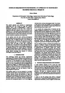


![Minimum Computer Requirements Guide - MATC [PDF]](https://m.moam.info/img/260x300/minimum-computer-requirements-guide-matc-pdf_6481c202098a9ea0088b4588.jpg)