May 2, 1987 - It was found recently that the jerk, the third derivative of position, of the desired trajectory, adversely affects the efficiency of the control al-.
M I N I M U M JERK PATH GENERATION
Konstantinos J. Kyriakopoulos George N. Saridis Department of Electrical, Computer and Systems Engineering Rensselaer Polytechnic Institute Troy, New Yoik 12180-3590
ABSTRACT
of this factor, and challenge the opinion of some researchers that jerk must always be continuous3. The free execution time o f a manipulation task has been used t o account for the velocity and acceleration constraints instead of the complete bounded state variable formulationz0. This approach yields simpler and more practical expressions for trajectory planning. Section 2 states the formulation o f the problem in joint space. Sections 3 and 4 solve i t for some cost criteria. In Section 5 the statement of the problem i n Cartesian space i s presented and analytical solutions for two criteria are given. Section 6 presents the resulting desired trajectories and gives on-line results. Finally in section 7 further research in this direction is suggested.
This paper presents a simple method o f trajectory generation of robot manipulators based on an optimal control problem formulation. It was found recently that the jerk, the third derivative of position, of the desired trajectory, adversely affects the efficiency of the control algorithms and therefore should be minimized. Assuming joint position, velocity and acceleration t o be constrained a cost criterion containing jerk is considered. Initially. the simple environment without obstacles and constrained by the physical limitations o f the joint angles only i s examined. For practical reasons, the free execution time has been used t o handle the velocity and acceleration constraints instead of the complete bounded state variable formulation. The problem o f minimizing the jerk along an arbitrary Cartesian trajectory i s formulated and given analytical solution, making this method useful for real world environments containing obstacles.
2. STATEMENT OF T H E PROBLEM The problem under consideration is expressed as: "Starting from an initial point i. in the joint space. definedby the joint angles vector, q ' , with 2 = 2 = 0. go t o the final point f defined by q', and q' = q' = 0. by minimizing a cost function J ( q , q , i,'q, T)",The execution time T IS free and i s specified in the above cost function i n order t o satisfy the inequality constraints on the states. Consequently, the joint position, velocity and acceleration for the i-th joint are expressed as state variables z i l rz ; ~z,3 , respectively, then
1. INTRODUCTION During the last two decades several control methods for robotic manipulators have been d e v e l ~ p e d ~ * " - ' ~ Most . of the already developed control methods indicate that the control of manipulators i s achieved in several sequential stages. One o f these stages i s trajectory planning, where a desired trajectory with prespecified position, velocity and acceleration i s necessary. In some o f these methods, in order t o calculate the input vector 7 ( k ) o f torques at instant k . the desired position at the instant k + 2 i s needed, making off-line trajectory generation necessary5. Several methods of trajectory planning have been developed in the 'z. methods assume a prespecified past y e a r s ' ~ 6 ~ 1 0 ~ 1 3 ~ 1 4 ~ 1 6 ~ ' 1 ~These path in Cartesian space that can be subsequently transformed by inverse kinematics. i n joint space as a set of points, each representing a specific configuration of the arm1>l5. Earlier method^'^^'^ assume that the preplanned path t o be traveled is composed o f straight line segments in Cartesian coordinates, connected by smooth arcs, while the other2~13~16~Z1~22 assume a general smooth Cartesian path. A real time technique for obstacle avoidances is presented in6, where the path generation problem is being done in the lower level o f a hierarchical control system. A generalized version o f the statement of the problem of trajectory planning is given inz1: "Given a curve i n the robot's joint soace. the robot's dynamic Drooerties. and the robot's characteristics, what set of sianals t o the actuators will drive the robot from its current state t o a desired final state w i t h a minimum cost?" The actuator's characteristics represent mainly torque constraints which can be expressed i n terms of bounds related t o torque, rather than torque itself. For example. a trajectory under constrained joint position, velocity acceleration and jerk is a sufficient trajectory for the input torques. The last term. jerk. has recently been defined a s a serious constraining factor for the trajectory planning problem. Some trajectory planning formulations simply report the resulting jerk from their methodsz3. while others attempt time-optimal solutions taking into account jerk constraints, thus producing bounded jerk trajectories". Experimental results i n the Robotics and Automation Labs of Rensselaer Polytechnic Institutes. have indicated that joint position errors are increasing when jerk increases. The present work yields desired trajectories, by minimizing a cost criterion containing jerk in a space free of obstacles. The results are interesting since they show the significance
iil(t) =
t ~ ( t )
i.,(t) = ' q , ( t ) = U; where jerk ' q , i s expressed a s an input U, t o the system. Doing the same for all n joints of the manipulator, a system describing the position. velocity and acceleration o f the manipulator is obtained, with the jerk as an input 0 0 0
1 0 0
0 1 0
0
0 1 0
0 0 1 0 0 0 0 0 0 1 ... ...
0 0
+
0 0 0 0 0 0 ...
0 0
... ... ...
0 0
1
...
... ... ... ...
...
..
..
0 0 0
0 0
1-
This system is obviously decoupled. consisting of n-subsystems of the form z,=A,z,+B,u, z - l , 2 , ...,n
364
CH2555-1/88/0000/0364$01.000 1988 IEEE
& ( t )= ~
= k ( t ) = 2i3(t)
&2(t)
where 2; =
and
Q
for some arbitrary admissible control ui(t). The costate equation i s
[q; q; q;1=
i s the input (jerk) for the i t h joint, and
ax = -ATpf(t)
f ( t ) = --
az,
w i t h e-ATt =
= e-Ar'p*(0)
*pf(t)
[
0 1 -t
with initial and final conditions
(3.3)
0 01
(3.4)
1
and
1'
Pi(0) = [ P i i ( o ) Piz(0) Pi3(0) (3.5) Substituting (3.5) and (3.4) i n t o (3.3) and subsequently t o (3.2) one obtains ai FJf&)uf(t) Iai Plt3(t) ' ui(t) (3.6)
where T represents the free execution time for the motion. The current problem i s a bounded state one, due t o the physical limitations o f the joints and actuators. as expressed by the equations q,(O) = qimin
+
I qs(t) = zil(t) I qimmsx = qi(T)
Pf3(t) = Pi3(0)
Iz.z(~) 2 V i m s x I& ( t )I = 1% ( t )I I 0; max Iqi(t)I =
- tPi2(0)
t2
+ TPil(0)
(3.7)
The minimum o f the right side o f (3.7) i s achieved for
(2.5)
In this analysis, a cost function containing only the jerk i s assumed. Therefore, a control i s sought that U;
+
where
u ' ( t ) = -a; . sgnpf3(t)
(34
The case where pf ( t ) . given by eq. (3.7). has one or no real roots i n [O,T]give no phy%al results. In the case of two real roots i n [O,T] these lie a t tl = and tz = 3T. between which pf3(0) < 0. Consider the solution o f (1.8) and the resulting trajectories i n the resulting time subintervals
E U 3 J(u)* I J(u)Vu E U
T
where U is the set o f admissible controls. A t this point a proper selection o f the minimizing criterion J(ui) i s necessary. In this work, solutions were obtained and gave desired trajectories that were tested on-line. for two kinds o f cost functions. The first was a %ax" type cost function
1.
[-:I
O t -uf(t) = a ;
&it) = a;t t2
and the second an input energy type cost function, used mainly for comparison purposes, since an approach based on that has been given in
q;(t) = a;-
I41
q ; ( t ) =a;-
2
t3
. T
II. [tl = Analytical solutions for these cost functions are presented i n the following t w o sections respectively.
T,
t2
(3.9)
6
-1
= 3T
4
uf ( t ) = a;
3. MINIMIZATION OF T H E M A X I M U M JERK FOR JOINT SPACE The following criterion minimizes the maximum value o f the jerk over the interval [0, TI:
(3.10) The above optimal control problem i s not trivial. Therefore, a more detailed solution which i s closely related to18.1Q is presented here. The solution of the problem without the position. velocity and acceleration constraints i s as follows: First, introduce the costate vector p;(t) = [pil@) p ; 2 ( t ) p;3(t)lT and the Hamiltonian
111.
[tz =
y ,TI uf ( t ) = a;
& i t )= a;t - a;T
T2
t2
Q,(t)=a;--a;Tt+a;2 2 t3 T q ; ( t ) = a;- - a,-t2 + a.-t '2 '2 6
Assuming that u , ( t ) i s bounded by some value a;:
13 96'
- -a,T3
(3.11)
The above equations were derived by applying the initial conditions &(O) = 0. assuming continuity o f q;,q;,and Q everywhere. and applying the final point conditions q,(T) = G(T) = 0. Applying the final point condition q;(T)= Si one obtains q;(O) = q ; ( O ) =
the Hamiltonian i s rewritten as
H ( z , , ~ , , u , , t=)a , + ~ T ( t ) A z , ( + t )~ T ( t ) B u , ( t )
si
a;= 32-
(3.1)
T3
The Pontryagins minimum p r i n ~ i p l e ' ~expressed . i n terms o f the optimal values indicated by *. yields
The set o f equations (3.9) - (3.12) give a complete solution, and the corresponding trajectories have been plotted i n figures 1-4. under the label "by minimizing max ( U / " . A complete study of the current problem requires consideration of the velocity and acceleration constraints. However, if time T i s free, the control u ( t ) may be selected t o avoid the joint velocity and acceleration
H(uf,pf,u:, t ) = a;+ pi' ( t ) . A zf ( t )+ pf ( t ). B . uf ( t ) 5 a;+ pfT( t ) . A . z,'(t)
+ pfT(t) . B .
U;(t)
(3.12)
(3.2)
365
of upper bounds V , and aimaxrespectively. The minimum execution time T may be obtained t o satisfy these constraints.
Trajectories representing the above equations have been plotted in figures
1-4. under the label "by minimizing
lT
u'dt".
Investigation of the joint velocity and acceleration constraints yield the value of the minimum execution time. Using (4.5)one can derive
and
or, combining (3.13)and (3.14).
> 2.4028
,
T > T , = m a x [ 2 8 2 8 ( S - ) a, ' max
2(s,)] vi m a x
'
(">
a, m a x
(3.15) and
and seeking a lower bound for an d i n k manipulator
T >
max T,
(3.16)
i = l ,...,n
This last equation (3.16)gives just a lower bound of execution time, t o satisfy the velocity and acceleration constraints of the joint actuators. However, this is a gross estimation of the minimum execution time for a specific task, since the relation between velocity and acceleration constraints, and the torque of the actuators is position dependent. T h e position constraints d o not affect the execution time T. because i f the initial and final values of the joint angles, obtained by inverse kinematics, are acceptable, the values of the intermediate joint position trajectory have t o lie between these t w o values. This can be easily verified either from equations (3.9)(3.10)(3.11)where we see that q,(t) . S, 3 0 V t c [ O , TI. or f r o m figure 1 where the joint position trajectory i s plotted.
1.875 (
or combining (4.6)and (4.7)
T > T, = max 1 . 4 0 2 8
+ P T A ~+; pTBu,
where Pr(0) = IP,l(O) P d O ) P , 3 ( 0 ) l T In order t o find u : ( t ) from (4.3) explicitly, the costate transition matrix e - A T t is first calculated
1 -t
0
01 1
(4.8)
(4.9)
5. JERK MINIMIZATION I N CARTESIAN SPACE T h e problems stated so far and their solutions. refer t o the case of joint space constrained only by the physical limitations of the robot's joint angles and not including possible obstacles. However, in a realistic environment obstacles exist constraining the working space. Therefore, usually a sequence of set points are given representing a collision-free path specified by Cartesian coordinates, orientation Euler angels and by manipulator configurations (left-right arm. u p or down elbow, flipped or non-flipped wrist, etc.). This sequence of set points is connected properly (e.g. spline functions or straight line segments) finally giving a trajectory .(A) where X is a parameter of the Cartesian trajectory (e.g. the length of the trajectory covered up t o a specific point). In the general case. the robot arm has t o follow a fixed path in Cartesian space given by
(4.1)
(4.3)
0
(4.7)
The remarks stated in the preceding section for this time lower bound are also valid here. In addition t o that. for the reasons expressed before.the position constraints do not affect the execution time.
2
[
rnax
*=l,n
and
e-ATt=
I)-"(
T>mawT,
= 0 =+-u : ( t ) = --BTp:(t) 1
a U.
2
and seeking a lower bound for an n-link manipulator
Applying Pontryagin's maximum principle"
E
,
(L) * , 1.874 vx A inax
4. T H E " M I N I M U M ENERGY" PROBLEM FOR JOINT SPACE T h e cost function (2.6)i s t o be minimized, for the system (2.2) with initial and final conditions (2.4)and under the inequality constraints (2.5). T h e solution of the problem without the constraints, is a s follows: Define the costate vector pi(t) = [pil(t) p i z ( t ) p,3(t)]T and the Hamiltonian
H ( z , , y , p , , t ) =U:
U
(4.4)
r = .(A)
= lPz(X) PY(X) Pz(X)
4(X) Q ( X ) OX,P,
The dynamics of the manipulator are represented by
+
+ G(q) + R(d) = 7
D(q)(i+ H ( q , dl
6pT(x(z) -.(A))
5 rmax
~ ( z -) rmmax 50
= [q? 0 0 q;
Zf =
[q; 0 0 9; 0 0
"
+
+ Bu'
,20
(5.10.1)
+ ( z ( r ) ) = z ( r ) - zf = 0
(5.10.2)
x ( z * ) = .(A')
(5.4)
while the final condition i s
where
z6A)
i. = Az'
w(z*)
Q ( z ( T ) )= z ( T ) - Zf = 0
(g6z-
+pT
L, w, x , f,r, twice continuously differentiable functions
is the desired
o]=
0 o...q:
Z)
6J'(u*,p*,z*,s*, p*,X*,p',u*) = 0 it results that for
U
+ BU- + L ( u ) } dt
and since
+ R(d).
where z is given a t (5.2)A , B . can be seen a t (2.1)and jerk trajectory. The initial conditions of the system are
- +))+
6pT(Az+ B u - z ) + p T ( A . 6 z +B~u 6i)I d t
(5.3)
~ ( z ) D(ql(i + H(q,d) + G(q) where The system equation IS 5 = Az+ Bu
+ f(sH + PT(+
- 7,
Therefore. the first variation is
where T,,, is a 6 x 1 vector containing the maximum torques that the actuators can apply. If we introduce also the state vector z as in (6.2). then
20
{rT(+)
+pT(Az
where D ( q ) is the inertia matrix H ( q , Q )are the Coriolis and Centrifugal terms G ( q ) is the Gravity term R(q),,is the viscous friction term q, q , q, 7 = 6 x 1 vectors representing the joint position, velocity. acceleration and torque. The dynamic contraints require that 7
I'
4=y T W r ) ) +
+ f(s')
- r,
(5.10.3) =0
p*(T) = u'(T)
(5.5)
(5.10.4) (5.10.5) (5.10.6)
. q L 0 OIT
Therefore, the statement o f the problem, expressed verbally in the introduction, can now be formulated mathematically as: "Find the optimal control input U* t o the system
(5.10.7) (5.10.8)
z = Az+ Bu
(5.6)
,ZO given
aL
-+p*
driving the system t o the terminal manifold expressed as in eq. (5.5)
Q(z(T)) = 0
aU
B=O
(5.10.9)
The above problem is a two point boundary value problem which has t o be solved numerically.
(5.7)
under the contraints
5.1 Minmax problem
x ( z ) = .(A)
Assuming that
and W(Z)
,
- r, 5 0
J(u) = l ' L ( u ) d t
+ f(s) = 0
The optimal input U* cannot be found by (5.10.9)since L is not twice differentiable. Using Pontryagin's maximum principal as in Section 3. one obtains
(5.9.a)
J(u*,p*,p*,p',X',s*,z*,u*)
f(s)= xb;sTe;s2 0
which eventually gives
and since
'0 0
0 0 1
ei =
n
where a >0 then define as the cost criterion
(5.10)
of the input (jerk)." The above problem is an optimal control problem which, in order t o be solved, the inequality constraint (5.9)has t o be equality by assigning w ( 2 ) - 7,
c
tyoy,,=1 I = a
by minimizing some cost function
where
T
t
the minimum is obtained i f
ith r o w
0 0 0
-
5.2 Weighted input problem
367
5 J(u*,p*,p*,p*,X*,S*,Z*,u)
If we assign as cost function
expected. Further research could be directed towards the numerical solution of the resulting equations and a more detailed solution including the joint angles constraints which have not been considered here, using a formulation involving the complete bounded state variable approach developed in2'. Additionally, other cost functions, as minimum time or functions of jerk should be considered for minimization.
then (5.10.9) gives
2Ru' + p * = B = 0 j U* = - - 1R - ' P * ~ B 2
ACKNOWLEDGEMENTS The authors would like t o express their gratitude t o Steve Murphy for his assistance. This work was supported under the NSF Grant DMC83-12179.
Therefore. minimum energy problem given in4 was treated in the n-th space. Notice the fact that the above formulation does not include joint angles constraints because it would introduce n more state variables complicating the solution more. This is suggested for further research.
REFERENCES [l] A . Bazerghi. A. A. Goldenberg. and J. Apkarian. "An Exact Kinematic Model of P U M A 4 0 0 Manipulator". IEEE Transactions on Systems, Man and Cybernetics, Vol. SMC-14. No. 3. May/June 1984. [2] J. E. Bobrow. S. Dubowsky and J. S. Gibson, "On the Optimal Control of Robotic Manipulators With Actuator Constraints", Proceedings of American Control Conference, pp. 782-787. June 1983. [3] M . Brady. "Trajectory Planning and Robot Motion: Planning and Control", Cambridge. MA: M I T Press, 1982. [4] Hollerbach. J. M.. "The Minimum Energy Movement for a Spring Muscle Model", Artificial Intelligence Laboratory, M.I.T.. AIM-424, 1977. [ 5 ] R. Horowitz and M . Tomizuka. "Discrete Time Model Reference Adaptive Control of Mechanical Manipulators". Computers in Engineering, 1982. Vol. 2. Robots and Robotics. ASME. pp. 107-112. [GI 0. Khatib. "Real-Time Obstacle Avoidance for Manipulators and Mobile Robots". Proceedings 1985 IEEE International Conference on Robotics and Automation pp. 5OC-505. [7] P. K . Khosla. "Real-Time Control and Identification or Direct-Drive Manipulators". Ph.D. Thesis, Department of Electrical and Computer Engineering, Carnegie Mellon University, August 1986. [ 8 ] M . B . Leahy and G. N. Saridis. "Compensation of Unmodeled PUMA Manipulator Dynamics". Proceedings 1987 IEEE International Conference on Robotics and Automation, pp. 151-156. [9] M . B . Leahy. "Development and Application of a Hierarchical Robotic Evaluation Environment". Ph.D. Dissertation, Robotics and Automation Labs, RPI. August 1986. [ l o ] J. Y. S. Luh and C. S. Lin. "Optimal Path Planning for Mechanical Manipulators". ASME Journal of Dynamic Systems. Measurement and Control, Vol. 102. pp. 142-151. June 1981. [ll] G. L . Luo and G. N. Saridis. "L-Q Design of PID Controllers for Robot Arms". IEEE Journal of Robotics and Automation. Vol. RA1. No. 3. September 1985 1121 B . R . Markiewicz. "Analysis of the Computed Torque Drive Method and Comparison with Conventional Position Servo for a Computed Controlled Manipulator". Technical Memo 33-601. JPL. March 1973. 1131 R. P. Paul, "Robot Manipulators: Mathematics, Programming and Control". Cambridge, M A : M I T Press, 1981. [14] R. Paul, "Manipulator Cartesian Path Control". IEEE Transactions on Systems, Man and Cybernetics, Vol. SMC-9. No. 11. Nov. 1979. pp. 702-711. [15] P. P. Paul, B . Shimano and G. E. Mayer. "Kinematic Control Equations for Simple Manipulators". IEEE Transactions on Systems, Man and Cybernetics, Vol. SMC-11. pp. 449-455. June 1981. [16] F. Pfeiffer and R. Johanni. "A Concept for Manipulator Trajectory Planning", IEEE Journal of Robotics and Automation, Vol. RA-3, No. 2. April 1987. pp. 115-123. [17] L . S. Pontryagin. V . Boltyanskii. R. Gamkrelidze and E. Mishehenko. The hfathematical Theory of Optimal Processes. lnterscience Publishers. Inc.. New York, 1962. [18] G. Saridis and Z. V . Rekasius. "Investigation of Worst-case Errors When Inputs and Their Rate of Change Are Bounded", IEEE Transactions on Automatic Control, Vol. AC-11. No. 2. April 1966. pp. 296-300. [19] G. Saridis, "Algorithms for Worst Error in Linesr Systems with Bounded Input and i t s Rate of Change". IEEE Transactions on Autotnatic Control, Vol. AC-12. No. 2. April 1967. pp. 203-207.
6. ON-LINE RESULTS Since numerical solutions for the Cartesian space problem have not been obtained yet. i n this section only the joint unconstrained space is considered in order t o validate the assumption for the negative effect of jerk on the performance of a manipulator. In order t o plot the trajectories resulting from the previous analysis and validate the claims made, consider the following motion of the end effector of the PUMA-600. which was actually tested on the P U M A 4 0 0 robotic manipulator of the Robotics and Automation Labs of Rensselaer Polytechnic Institute. Initial Condition i p; = [ 0
0.4
n , = [ ~o 0, =
[-1
a; = [ O
0.21'
-11' 0
01'
1 01'
Final Condition f
I
p j = 0.4 n,
=IO
0,
=[-1
aj = [ O
-0.2IT
0.4
o
-11' 0
01'
1 01'
The minimum execution time for the case of minimum energy problem i s found from (4.8). T2 = 1.375 sec. while for the case of minmax problem i s found from (3.15). 2'7 = 1.4667 sec. Therefore, we selected T = 1.8 sec. The trajectories and the errors of joint 2 were considered a s representative and were plotted in Figures 1-5. In order t o compare the resulting "optimal" trajectories, two more trajectories were considered. The first plotted under the label "Cartesian triangular acceleration profile", follows a straight line between the initial and final point, with a Cartesian acceleration having a triangular profile, starting and finishing with zero Cartesian velocity and acceleration, which for a configuration with nonsingular Jacobian are translated t o zero joint velocity and acceleration for all joints: something desirable for the actuators. The second. plotted under the label "simple Cartesian straight line", is a constant Cartesian velocity straight line trajectory having. a s a matter of fact, large jerk a t the beginning and the end of the trajectory. The trajectories were tested using a computed torque/PID controller and the position errors can be found in Figure 5. The superiority of the "optimal" trajectories is obvious, especially for the intervals where the other have large jerk. However, the performance of the trajectory with "Cartesian triangular acceleration profile" is considered very satisfactory.
7. CONCLUSIONS The error analysis of Section 6 demonstrated the significance of jerk and the optimality of our results. Jerk affects adversely the performance of the actuators and has t o be minimum. The mathematical analysis and solution for the unconstrained joint space problem was given t o given an insight of the problem and also t o verify the assumptions on the significance of jerk. However, due t o the fact that in a realistic environment the robot has t o follow an arbitrary Cartesian trajectory, in order t o satisfy the obstacle avoidance specifications, this problem was stated and theoretically solved. In this case of a general Cartesian trajectory the optimal control problem was reduced t o a two-point boundary value problem as
368
(201 G. N. Saridis and Z. V. Rekasius, "Design of Approximately Optimal Feedback Controllers for Systems of Bounded States". IEEE Transactions on Automatic Control. Vol. AC-12. No. 4. August 1967. pp. 373-379. [21] K. G. Shin and N. D. McKay. "Automatic Generation o f Trajectory Planners for Industrial Robots", Proc. 1986. IEEE Conference on Robotics and Automation, pp. 260-266. April 1986. [22] K . G. Shin and N. D.McKay. "Minimum-Time Trajectory Planning for Industrial Robots with General Torque Constraints", Proc. 1986. IEEE Conference on Robotics and Automation, pp. 412-417. April 1986. [23] S . E. Thomson. R. V. Patel. "Formulation of Joint Trajectories for Industrial Robots Using B-Splines" , IEEE Transactions on Industrial Electronics, Vol. IE-34. No. 2. May 1987. pp. 192-199.
Position 0
-
0
' o oa
Trajectory rlrplc cart c l 1 trlang
0 53
~ C Ci i r o f l l e
Figure 3.
0 hy nlnlllilng narlul P
1.60
I37
13
TlmelSec)
ItT 11°C
by ainlmlzlnQ Tu2'dt
Desired Acceleration Trajectory for Joint 2
Jerk Trajectory
-
0
by .Inlmlilng
, ju""dt line
Q r i s r i c c a r 1 sir Q
i r t trlanp acc profile
13
Figure 1.
Differential Desired Position Trajectory wrt to Initial Angles for Joint 2
Velocity
Figure 4.
Trajectory
rlmple c a r t sir Ilnc Q c r t t r h n g acc p r o f l h 0
Resulting Jerk Trajectory for Joint 2
P o s i t i o n Error o
0 by i l n l l l l l n Q m x b l
siaplccart sir llne prolllr
Q crt r r l a n g a m
by m l n l n l z l n g ) z ~ d t
0
3
Figure 2 .
Desired Velocity Trajectory f o r Joint 2
Figure 5.
369
On-Lme
Position Errors for Joint 2