Seasonal trends and weekday/weekend effects were investigated. Conditional ...... Polissar, A. V., P. K. Hopke, and R. L. Poirot (2001), Atmospheric aerosol.
JOURNAL OF GEOPHYSICAL RESEARCH, VOL. 110, D07S19, doi:10.1029/2004JD004707, 2005
Mining airborne particulate size distribution data by positive matrix factorization Liming Zhou,1 Eugene Kim, and Philip K. Hopke Center for Air Resources Engineering and Science and Department of Chemical Engineering, Clarkson University, Potsdam, New York, USA
Charles Stanier2 and Spyros N. Pandis Department of Chemical Engineering, Carnegie Mellon University, Pittsburgh, Pennsylvania, USA Received 28 February 2004; revised 13 July 2004; accepted 2 August 2004; published 17 March 2005.
[1] Airborne particulate size distribution data acquired in Pittsburgh from July 2001 to
June 2002 were analyzed as a bilinear receptor model solved by positive matrix factorization (PMF). The data were obtained from two scanning mobility particle spectrometers and an aerodynamic particle sampler with a temporal resolution of 15 min. Each sample contained 165 size bins from 0.003 to 2.5 mm. Particle growth periods in nucleation events were identified, and the data in these intervals were excluded from this study so that the size distribution profiles associated with the factors could be regarded as sufficiently constant to satisfy the assumptions of the receptor model. The values for each set of five consecutive size bins were averaged to produce 33 new size intervals. Analyses were made on monthly data sets to ensure that the changes in the size distributions from the source to the receptor site could be regarded as constant. The factors from PMF could be assigned to particle sources by examination of the number size distributions associated with the factors, the time frequency properties of the contribution of each source (Fourier analysis of source contribution values), and the correlations of the contribution values with simultaneous gas phase measurements (O3, NO, NO2, SO2, CO) and particle composition data (sulfate, nitrate, organic carbon/ elemental carbon). Seasonal trends and weekday/weekend effects were investigated. Conditional probability function analyses were performed for each source to ascertain the likely directions in which the sources were located. Five factors were separated. Two factors, local traffic and nucleation, are clear sources, but each of the other factors appears to be a mixture of several sources that cannot be further separated. Citation: Zhou, L., E. Kim, P. K. Hopke, C. Stanier, and S. N. Pandis (2005), Mining airborne particulate size distribution data by positive matrix factorization, J. Geophys. Res., 110, D07S19, doi:10.1029/2004JD004707.
1. Introduction [2] There have been many studies that find relationships between elevated morbidity and mortality and higher particulate matter (PM) concentrations [Dockery and Pope, 1994; Pope et al., 1995; Brunekreef et al., 1995; van Bree and Cassee, 2000]. In order to develop an effective control strategy for airborne particles, the relationship between the sources and receptor concentrations needs to be understood. [3] Positive matrix factorization (PMF) is a powerful tool for solving receptor models with aerosol composition data and has been used successfully in identifying the sources of the airborne particles in many studies [Xie et al., 1999; Lee 1 Now at Providence Engineering and Environmental Group LLC, Baton Rouge, Louisiana, USA. 2 Now at Department of Chemical and Biochemical Engineering, University of Iowa, Iowa City, Iowa, USA.
Copyright 2005 by the American Geophysical Union. 0148-0227/05/2004JD004707$09.00
et al., 1999; Ramadan et al., 2000; Chueinta et al., 2000; Polissar et al., 2001; Song et al., 2001]. Recently, the aerosol size distribution data have been analyzed by principal component analysis [Ruuskanen et al., 2001; Wahlin et al., 2001] and PMF [Kim et al., 2004]. [4] It is obvious that particles in different size ranges have unique characteristics and one always needs to consider classifying the size range before detailed analyses. A threemodal structure was widely used to describe continental particle number size distribution, including a nucleation mode at 10– 20 nm, an Aitken mode at 40– 80 nm, and an accumulation mode at 100– 300 nm [Whitby, 1978; Raes et al., 1997; Hussein et al., 2004]. Lognormal distribution functions representing the three modes were used to parameterize size distribution, and the modes fit by the lognormal distribution functions were thought to be associated with particle sources and processes during the transport [Birmili et al., 2001]. Using constant modal distribution functions was also proved possible if particle growth processes from nucleation mode to Aitken or even accumulation mode were
D07S19
1 of 15
D07S19
ZHOU ET AL.: MINING PARTICLE SIZE DISTRIBUTIONS
not considered [Ma¨kela¨ et al., 2000]. It is worth mentioning that for size distributions with a stable structure, using variant modal distributions instead of constant ones tends to be an overfitting, which means that the small random variations of the modes and even measurement errors may be fit and, consequently, the features of the modes may be smeared. [5] The Pittsburgh supersite was located in a strong anthropogenic source region, and the size distribution measured there cannot be fit well by the aforementioned threemodal distribution [Stanier et al., 2004c]. Thus some other methods need to be applied for classifying the size ranges. [6] Previously, size distribution data from July 2001 measured by the Pittsburgh Air Quality Study (PAQS) have been analyzed to identify the particle sources by PMF [Zhou et al., 2004]. Five sources were identified: secondary aerosol (from distant sources), local stationary combustion, remote traffic (probably from the interstate highway 1 mile away), local traffic (from the street and minor roads close to the receptor site), and nucleation, with decreasing sizes. The PMF method has successfully divided the particles into the five classes on the basis of both their size ranges and temporal behavior without prior assumptions such as lognormal distribution and the number of modes. The PMF analysis requires stationary or quasistationary size distributions measured at the receptor site. In a short period such as one month, conditions that might affect particle size changes such as photochemical activity or temperatures may be taken as relatively constant, and the change of the particle size distribution can be thought to be sufficiently constant to permit the PMF analyses. [7] Our recent study has indicated linear relationships between size distribution data and chemical composition data simultaneously measured at the Pittsburgh supersite [Zhou et al., 2005], and this is a direct proof of the stationarity of the size distribution. [8] In this study, a larger data set from PAQS, containing 1 year of size distribution data from July 2001 to June 2002, has been analyzed for source identification. Data mining is a process to discover patterns and relationships in data using various tools. The tools used in this study, including PMF, will be introduced in the next sections. Each factor found by PMF can be thought of as a pattern that represents the variations of a source or a group of sources. The possible sources associated with each factor (or pattern) will be investigated. [9] Over a full year the atmospheric processes influencing the size distributions vary significantly, and our previous efforts in directly analyzing the full year data set proved to be inappropriate [Zhou et al., 2003]. Therefore this analysis will be performed on a month-by-month basis. [10] In our previous work [Zhou et al., 2004], the days with extensive nucleation events, especially those events followed by particle growth, were excluded, and this leads to an incomplete description of the summer situation at the Pittsburgh area. In this study, a special method has been designed to remove only the data representing particle growth events, and thus a more thorough and complete investigation will be made.
2. Description of the Data [11] The receptor site was located in Schenley Park, Pittsburgh (latitude 40.4395�, longitude �79.9405�). An
D07S19
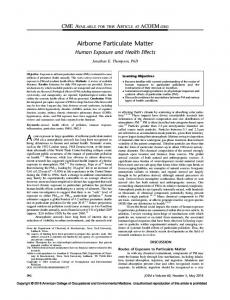
Figure 1. Typical particle growth on 2 July 2001.
overall summary and preliminary results for PAQS were given elsewhere [Wittig et al., 2003]. The size distribution data were obtained from July 2001 to June 2002. Samples were collected and measured continuously every 15 min. The data were from two scanning mobility particle spectrometers (SMPS) and an aerodynamic particle sampler (APS). Above 583 nm, the data used in this study represent the electrical mobility diameter inferred from aerodynamic mobility and estimated density [Khlystov et al., 2004]. The ratio of APS diameter and SMPS diameter is around 1.3. The samples were collected at 25% relative humidity, and ‘‘dry’’ particle distributions were obtained [Stanier et al., 2004a]. [12] The gas phase concentrations (O3, NO, NOx, SO2, and CO, with a 10 min resolution), particle mass and composition (PM2.5, sulfate, and nitrate, with 10 min time resolution; organic carbon (OC) and elemental carbon (EC), with 2 to 4 hour resolution), and meteorological conditions (wind direction, wind speed, etc., with 10 min resolution) were measured at the same time and location as the size distribution data. A detailed description of the instrument and sampling methods can be found elsewhere [Wittig et al., 2003; Stanier et al., 2004b]. Each size distribution sample contained 165 geometrically equal sized intervals covering the particle size range of 0.003 – 2.5 mm.
3. Exclusion of Data Representing Particle Growth [13] Nucleation events observed at the Pittsburgh site were classified as regional and short-lived by Stanier et al. [2004b]. In a regional nucleation event, it is often observed that the newly formed particles continue growing. Particle growth events are confined to limited time intervals and size ranges from over 10 nm up to accumulation mode size. A typical growth event after the nucleation is shown in Figure 1, where the number concentrations on 2 July 2001 are shown. These particle growth events were also observed at many other places, and the experimental and theoretical studies on this phenomenon were recently reviewed by Kulmala et al. [2004]. Discussions of the mechanisms of these events are beyond the scope of this study.
2 of 15
ZHOU ET AL.: MINING PARTICLE SIZE DISTRIBUTIONS
D07S19
D07S19
Figure 2. Number concentration and mean size variations on 2 July 2001.
[14] Receptor models require that the property being apportioned be stationary or, in this case, that there must be constant size distribution profiles associated with all factors. The temporal variations of the size distribution caused by particle growth events will deform the model solutions and make the sources unidentifiable. Particle growth during a regional nucleation event was identified, and the data representing the growth were removed by the following method. The number-concentration-weighted mean diameter is defined by the following equation: log dav ¼
X � � X � � N dp log dp = N dp : dp
ð1Þ
dp
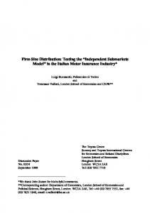
In addition to the variation of number concentration dN/dt, the number-concentration-weighted diameter can also be used to investigate the nucleation event. If there is a nucleation event, the number concentration increases sharply, and the mean diameter should simultaneously drop sharply since the newly formed particles have the smallest sizes and the largest number concentrations. [15] Since many particle growth events occurred in the size range above 6 nm, the total number concentration and mean diameter above 6 nm, N6 and dp6,av, were used. Here, N6 is the total number concentration over 6 nm; dp6,av is computed by equation (1) for all particles larger than 6 nm. The beginning of particle growth is defined quantitatively as the point at which no significant decrease of mean diameter occurs when the number concentration has a sharp increase and the mean diameter rises gradually afterward. In Figure 2, t1 is found to be the start of particle growth. The mean diameter dp6,av does not change with time when particle growth becomes stable. A polynomial regression of log dp6,av against time
was made to estimate the time after which the variation in mean diameter is sufficiently small, as shown in Figure 2. When the first derivative of the regressed value is below a criterion value, such as at t2 in Figure 2, the growth can be considered to have terminated. [16] By assuming the number concentration distribution versus dp6,av to be lognormal (during the particle growth after the nucleation, the number concentration distribution over 6 nm is usually unimodal), we define the data, within ±1.2s from the regressed dp6,av and between t1 and t2, representing particle growth, where s is the standard deviation of the lognormal distribution for each time interval. Figure 3 shows the result of this definition for 2 July 2001. The data thus defined were treated as missing values, which means replacing these values by the mean values and
Figure 3. Definition of particle growth zone for 2 July 2001.
3 of 15
ZHOU ET AL.: MINING PARTICLE SIZE DISTRIBUTIONS
D07S19
Table 1. Days With a Particle Growth Zone Defined (Data by This Definition Excluded in PMF Analysis) Month
Days
July 2001 Aug. 2001 Sept. 2001 Oct. 2001 Nov. 2001 Dec. 2001 Jan. 2002 Feb. 2002 March 2002 April 2002 May 2002
2, 11, 14, 15, 24, and 30 July 7, 11, 14, and 18 Aug. 1, 5, 11, 14, 16, and 26 Sept. 7, 10, 11, 15, 18, 20, 24, 25, 29, and 30 Oct. 3, 4, 8, 9, 10, and 22 Nov. None 25 and 26 Jan. 13, 14, and 25 Feb. 6, 7, 9, 15, 23, 24, and 29 March 2, 10, 11, 12, 16, 17, 18, and 19 April 4, 5, 10, 11, 15, 16, 17, 23, 24, 26, 27, 28, 29, 30, and 31 May 2, 3, 4, 5, 8, 9, 21, 22, 23, 24, and 29 June
June 2002
seen that this kind of particle growth phenomenon rarely happened in winter.
4. PMF and Other Tools for Mining the Size Distribution Data 4.1. PMF [17] A detailed introduction to PMF can be found elsewhere [Paatero, 1997]. In this study, PMF2 (two-way PMF) is used to solve the following two-way receptor model: X ¼ GF þ E
ð2Þ
or, in the elemental form, xij ¼
assigning them high uncertainties (low weights), such as 10 times their concentrations. Thus these data will not influence the PMF result and will not be reflected in the factors obtained by PMF. The data before and after this operation were inspected visually, and sometimes the parameters were adjusted manually to properly define the particle growth zone. If a regional nucleation event is followed with no particle growth, the corresponding data were not processed by this method. The days processed by this method are listed in Table 1. From this table, it can be
D07S19
p X
gik fkj þ eij ;
ð3Þ
k¼1
where X is the matrix of observed data and the element xij is the number concentration value of the ith sample at the jth size bin. G and F are the source contributions and size distribution profiles, respectively, of the sources that are unknown and to be estimated from the analysis. To be specific, gik is the concentration of particles from the kth source associated with the ith sample and fkj is the size distribution associated with kth source. E is a matrix of residuals.
Table 2. Description of the Whole Year Data (Data Representing Particle Growth Excluded) Number Concentration, number cm�3 Min
Max, � 103
Median, � 103
Lower 25%, � 103
Upper 25%, � 103
Mean Volume Concentration, mm3 cm�3
0 0 0 0 0 0 0 0 0 0 0 0 0 0.6 0.44 0 0 0 0 0 0 0 0 0 0.32 0 0 0 0.43 1.81 0.23 0.1 0
1550 496 241 306 667 2110 406 304 405 688 481 371 1170 444 224 150 131 124 118 96.9 51.8 38.0 23.5 19.2 19.0 11.0 5.9 4.1 2.6 0.84 0.21 0.054 0.036
7.8 5.7 5.4 5.9 6.9 8.3 10.1 11.5 12.6 12.0 12.3 12.3 12.7 13.4 13.7 13.6 12.6 11.2 9.8 8.5 6.9 5.3 3.8 2.6 1.7 0.98 0.51 0.22 0.089 0.056 0.0075 0.00190281 0.0009
0 0 2.4 3.2 3.9 4.9 5.8 6.7 7.2 6.9 7.2 7 7.5 7.8 7.7 7.6 7.2 6.7 6.0 5.1 4.1 3.3 2.5 1.7 1.1 0.62 0.29 0.12 0.045 0.027 0.0037 0.0012 0.0007
23 13 10 9.7 10 12 13 15 16 17 17 17 18 20 19 19 17 15 13 11 9.3 7.3 5.7 4.1 2.7 1.7 0.96 0.45 0.19 0.109 0.12 0 0.0013
0.00038 0.00034 0.00045 0.00074 0.0013 0.0026 0.0050 0.0096 0.018 0.030 0.056 0.10 0.18 0.31 0.54 0.90 1.4 2.2 3.2 4.7 6.6 8.8 11 13 15 16.5 16 14 11 11 3.8 2.3 3.6
a
Size, mm
Mean, � 103
SD, � 103
0.0032 0.0039 0.0046 0.0055 0.0066 0.0079 0.0095 0.0113 0.0136 0.0163 0.0195 0.0233 0.0279 0.0334 0.0400 0.048 0.057 0.069 0.082 0.098 0.118 0.141 0.169 0.20 0.24 0.29 0.35 0.41 0.50 0.63 0.90 1.29 1.84
21.5 11.2 8.8 8.4 8.8 9.9 11.2 12.6 13.7 14.3 14.6 15.0 15.5 16.1 16.2 15.6 14.6 13.0 11.2 9.5 7.8 6.03 4.43 3.11 2.09 1.31 0.74 0.37 0.16 0.087 0.01 0.0021 0.0011
53 21 12.7 10.1 9.7 14 9.1 9.6 10.4 12.5 12.7 13.3 15.1 13.9 13.2 12.0 10.8 9.6 8.1 6.7 5.2 3.87 2.74 1.90 1.36 0.99 0.68 0.41 0.21 0.092 0.010 0.0018 0.0009
a
SD, standard deviation.
4 of 15
ZHOU ET AL.: MINING PARTICLE SIZE DISTRIBUTIONS
D07S19
D07S19
Figure 4. Histograms of the scaled regression residuals. The horizontal axes indicate the scaled residual, and the vertical axes indicate the frequencies.
[18] The residual sum of squares (Q) is minimized by finding the optimal F and G values as indicated in equations (2) and (3): � � X X �eij �2 �ð X � GF Þ�2 � Q¼� ¼ : � � sij s F;G j i
ð4Þ
[19] Rotations are obtained by setting an FPEAK value [Paatero et al., 2002]. When the FPEAK value is positive, the following additional term is included in the object function Q: P
Q ¼b
2
p X n X
!2 fkj
;
ð5Þ
k¼1 j¼1
where b2 corresponds to the FPEAK value. The term defined above attempts to pull the sum of all the elements of F toward zero and makes the program do elementary transformations for F and G by subtracting the F vectors from each other and adding corresponding G vectors to obtain a more physically realistic solution. Recently, a method for solving rotational ambiguities by detecting edges in G space have been developed, and the best solution is obtained without clearly defined edges in G space [Paatero et al., 2005]. In this study, the FPEAK
value is set to 0.2 for each of the months to eliminate G space edges, and five similar factors were found for each month. [20] The F values were normalized to make the sum of each size interval equal to 1 for each factor. The G values were then rescaled correspondingly. The uncertainties were estimated with the method described by Zhou et al. [2004]. To smooth the size distribution data and minimize the error caused by the discontinuity between instruments, every five consecutive size bins were combined into one, and 33 new size intervals were produced from the original 165 size bins. The analysis of volume size distribution data does not provide much more information since it generates similar source contributions as number size distribution analyses do [Zhou et al., 2004], and hence it will not be performed in this study. During the period between October 2001 and April 2002 the APS was not working, and only 29 new size intervals were produced for these months. This also caused incomplete information on volume size distribution. Table 2 summarizes the data set after the aforementioned treatment. 4.2. Correlation Analyses [21] Correlations of some compositions and gases with source contributions were investigated. Using only gas data as an input to PMF will not bring much more information, and both data sets need to be averaged to 30 min. The 15 min resolution has made possible a more thorough time series
5 of 15
ZHOU ET AL.: MINING PARTICLE SIZE DISTRIBUTIONS
D07S19
D07S19
Figure 5. Size distribution profiles for each month.
analysis than 30 min resolution, such as in the time of day effect. 4.3. Conditional Probability Function (CPF) [22] A conditional probability function [Ashbaugh et al., 1985; Kim et al., 2004] was calculated using the source contributions obtained by PMF2 and wind direction values by the following equation: CPF ¼
mDq ; nDq
ð6Þ
where mDq is the number of occurrences in the direction sector that exceeds the threshold, upper 25th percentile of the fractional contribution from each source, and nDq is the total number of wind occurrences in the same direction sector. Fractional contributions are used to avoid the influence of atmospheric dilution on CPF results. The angular width of direction sector is set as 10�, and thus there are 36 directional sectors. Those samples corresponding to a wind speed below 1.0 m s�1 are excluded from this study, and two thirds of the total samples were excluded. The sources are thought to be located in the direction sectors
6 of 15
D07S19
ZHOU ET AL.: MINING PARTICLE SIZE DISTRIBUTIONS
Figure 6. Discussion of the two modes of factor 1 in July 2001. (a) Size distribution of factor 1. (b) Scatterplot of the number concentration of the central size intervals of the two modes. with high CPF values. When nDq is below 10, the CPF value is set to zero. 4.4. Fourier Analysis [23] The source contributions from each month are linked in a temporal sequence to form annual source contribution series, and Fourier analyses have been performed for these annual series. In the signal-processing field, it is well known that Fourier analysis has no temporal specificity. For example, if the Fourier analysis says that the series has a daily pattern (24 hour period), it cannot determine that the daily pattern exists at any specific time in the series. Therefore many time-frequency analysis techniques have been developed and used in combination with Fourier analyses. To address the problem in this study, the Fourier analysis was performed for the source contributions of each month. The correlations of the source contributions with the gas and particle composition data were calculated for each month.
5. Results and Discussion [24] Table 2 describes the average number and volume size distribution of the full year of data. The volume distribution mode is located between 0.1 and 1 mm. The smallest particles
D07S19
have the largest mean number concentration, but their median concentrations are not the highest. This situation may be caused by the frequent nucleation events that produce large numbers of new particles. Table 2 also indicates that the minimum number concentrations in all the size intervals are nearly zero, implying very low contributions from certain sources. The 12 months of data were summarized and described in detail elsewhere [Stanier et al., 2004c]. Figure 4 indicates the histograms of the scaled regression residuals for all size intervals of all 12 months. Most of the residuals are within �2 and +2, and the distributions are symmetric and close to normal distributions. If the size distributions measured at the receptor are not stationary or quasistationary, then these good regressions cannot be obtained. The five factors are arranged in order of decreasing size from factor 1 to factor 5. These five factors are similar to the sources identified in our previous study [Zhou et al., 2004]. Detailed discussion is provided as follows. [25] Factor 1 has a number mode between 0.15 and 0.25 mm and a submode at 0.02 mm, as shown in Figure 5. Detecting edges in F space is a method to help resolve rotation problems [Henry, 2003]. For July 2001 the number concentrations of the two size intervals d1 (240 nm) and d2 (23 nm), the center size intervals of the two modes, were plotted in Figure 6. The edge corresponding to FPEAK = 0.2 was also plotted. When pulling down the submode by increasing the FPEAK value, the edge will rotate toward the d1 axis, but it is clear that the edge cannot overlap with the d1 axis, suggesting that the submode cannot be eliminated completely. Nevertheless, for the solutions with different rotations, the major mode and source contributions did not experience large changes, and our analysis and conclusions were not severely influenced. [26] In Figure 7, the Fourier analysis shows a weak daily pattern for factor 1. Table 3 indicates that the daily pattern is clear in February and April of 2002 but not that clear in other months. Fourier analyses have also been applied for sulfate and nitrate data for each month. These analyses found that sulfate does not have daily patterns except in the summer months (it had weak daily patterns in July and August of 2001 and June of 2002) and nitrate usually has a strong diurnal pattern during the whole year except in November and December of 2001 and January and March of 2002. On the basis of these facts, one possible explanation for the periodicity of factor 1 is as follows: When the sulfate concentration is low and nitrate has a strong simultaneously diurnal pattern, such as the situation of February and April of 2002, the temporal behavior of factor 1 can be influenced by nitrate and shows observable daily patterns. Another possible reason is that some local emissions have been included in factor 1. However, the reason cannot be completely clarified within the current data sets. [27] Factor 1 has a strong correlation with PM2.5 mass over the entire period as indicated in Table 4 and is related to the major components of the PM2.5 mass at the Pittsburgh supersite. In winter the correlation of nitrate with factor 1 increases, suggesting that more nitrate is included in factor 1. [28] As indicated in Table 4, factor 1 usually has high correlations with sulfate. Secondary sulfate was formed by the oxidation of SO2 through photochemical reactions.
7 of 15
D07S19
ZHOU ET AL.: MINING PARTICLE SIZE DISTRIBUTIONS
D07S19
Figure 7. Fourier transformation for the annual contribution of each factor. (The powers are all nearly zero for all factors from 0.2 h�1 to 2 h�1, the Nyquist frequency.) The main SO2 sources are coal-fired power plants hundreds of kilometers away. In winter the correlation of factor 1 with nitrate increases noticeably. The lower temperatures support ammonium nitrate in the solid phase, and the fraction of nitrate in PM2.5 mass increases. The increase of the correlation coefficient with nitrate may explain the higher correlation of factor 1 with PM2.5 than with sulfate during winter, and this is also consistent with the fact that there was much less sulfate in winter. [29] Factor 1 has a higher correlation with OC than with EC in the summer and fall of 2001, but the correlations are similar for both species in the first half of 2002. The higher correlation with OC than with EC in the summer may be caused by secondary organic matter condensing onto preexisting particles during the transport as well as more production of secondary OC in the summer. When primary OC dominates, the correlations with OC and with EC are similar since they are from the same sources and have similar temporal variations. In Figure 8 the CPF analysis shows that factor 1 is from the south. Table 5 summarizes the characteristics of factor 1 and other factors. [30] Factor 1 typically includes sulfate, nitrate (in winter), and secondary organics as well as primary organics that have aged in the atmosphere and have grown from their original size. The particles of the submodes cannot be from distant places; otherwise, they would be depleted during the transport. The small modes of factor 1 are more likely to be from fresh emissions of some combustion sources south of
the site. Since the dominating direction of factor 1 is south, the particles of the small mode have the same variations as other large particles in factor 1, which may explain the correlation with CO. Factor 1 includes secondary, aged primary aerosol particles and also fresh primary particles from local combustion sources. [31] The number mode of factor 2 is at 0.08 � 0.1 mm in July, August, and September of 2001. In 2002 the number mode is at 0.06 � 0.07 mm. In Figure 9 a daily pattern, caused by the reduction of mixing height at night, is clearly observed. The nocturnal increase of the source contribution, owing to the reduction of the mixing height, may be the Table 3. Results of Monthly Fourier Analysis for Daily Patternsa July 2001 Aug. 2001 Sept. 2001 Oct. 2001 Nov. 2001 Dec. 2001 Jan. 2002 Feb. 2002 March 2002 April 2002 May 2002 June 2002
Factor 1
Factor 2
Factor 3
Factor 4
Factor 5
no no very weak very weak no no no weak no weak no no
weak no very weak weak very weak no no very weak no weak weak weak
no no no no no no no no no no no no
strong strong strong strong strong strong strong strong strong strong strong strong
strong strong strong strong strong strong strong strong strong strong strong –
a The strength of the daily patterns was decided by comparing the spectral intensity at 1/24 h�1 with other frequencies.
8 of 15
ZHOU ET AL.: MINING PARTICLE SIZE DISTRIBUTIONS
D07S19
D07S19
Table 4. Correlations r of the Source Contributions With Gas and Particle Composition Dataa O3
NO
NOx
SO2
CO
PM2.5
Sulfate
Nitrate
OC
EC
0.87 0.75 0.80 0.73 0.90 0.81 0.70 0.91 0.88 0.73 0.85 0.82
0.85 0.54 0.78 0.75 0.68 0.47 0.48 0.61 0.62 0.58 0.74 0.63
0.23 0.29 0.46 0.61 0.40 0.54 0.67 0.54 0.57 0.45 0.31 0.31
0.63 0.56 –b 0.67 0.89 0.74 0.56 0.82 0.65 0.51 0.80 0.58
0.28 0.42 –b 0.56 0.67 0.76 0.55 0.76 0.69 0.43 0.66 0.56
July 2001 Aug. 2001 Sept. 2001 Oct. 2001 Nov. 2001 Dec. 2001 Jan. 2002 Feb. 2002 March 2002 April 2002 May 02 June 02
0.18 �0.02 0.10 0.03 �0.05 �0.47 �0.42 �0.53 �0.50 �0.33 �0.12 0.18
0.03 0.20 0.26 0.32 0.42 0.46 0.51 0.70 0.43 0.44 0.39 0.13
0.18 0.29 0.34 0.41 0.48 0.45 0.56 0.75 0.57 0.52 0.45 0.35
0.16 0.07 0.21 0.27 0.33 0.14 0.17 0.34 0.30 0.18 0.22 0.17
Factor 1 0.19 0.42 0.38 0.51 0.57 0.61 0.47 0.76 0.59 0.52 0.50 0.49
July 2001 Aug. 2001 Sept. 2001 Oct. 2001 Nov. 2001 Dec. 2001 Jan. 2002 Feb. 2002 March 2002 April 2002 May 2002 June 2002
�0.18 �0.15 �0.24 �0.46 �0.51 �0.46 �0.37 �0.61 �0.50 �0.41 �0.29 �0.21
0.47 0.34 0.60 0.66 0.74 0.53 0.59 0.71 0.53 0.50 0.60 0.36
0.57 0.48 0.73 0.78 0.79 0.53 0.71 0.78 0.68 0.59 0.68 0.58
0.48 0.32 0.32 0.46 0.42 0.36 0.44 0.58 0.59 0.48 0.47 0.27
Factor 2 0.54 0.35 0.77 0.56 0.79 0.67 0.59 0.70 0.61 0.54 0.64 0.61
0.29 0.25 0.61 0.46 0.48 0.81 0.72 0.79 0.70 0.49 0.65 0.45
0.15 0.23 0.52 0.23 0.23 0.47 0.61 0.56 0.57 0.46 0.41 0.19
0.54 0.31 0.58 0.61 0.34 0.40 0.45 0.38 0.43 0.34 0.38 0.52
0.46 0.31 –b 0.43 0.41 0.80 0.71 0.66 0.53 0.36 0.64 0.50
0.56 0.39 –b 0.58 0.75 0.81 0.71 0.71 0.61 0.34 0.71 0.58
July 2001 Aug. 2001 Sept. 2001 Oct. 2001 Nov. 2001 Dec. 2001 Jan. 2002 Feb. 2002 March 2002 April 2002 May 2002 June 2002
�0.24 �0.27 �0.31 �0.24 �0.32 �0.25 �0.20 �0.23 �0.32 �0.28 �0.21 �0.17
0.37 0.32 0.36 0.39 0.33 0.20 0.38 0.16 0.35 0.30 0.33 0.22
0.40 0.44 0.51 0.45 0.36 0.18 0.42 0.20 0.42 0.37 0.41 0.30
0.23 0.18 0.29 0.24 0.15 0.34 0.40 0.45 0.52 0.59 0.49 0.21
Factor 3 0.28 0.31 0.43 0.22 0.21 0.24 0.30 0.08 0.28 0.28 0.27 0.20
�0.14 �0.01 0.13 0.13 0.04 0.34 0.28 0.11 0.31 0.22 0.15 0.02
�0.23 �0.11 0.07 0.02 �0.15 0.13 0.41 0.19 0.36 0.19 0.01 �0.05
0.23 0.25 0.30 0.28 0.17 0.31 0.35 0.10 0.22 0.17 0.11 0.20
�0.04 0.14 –b 0.08 �0.07 0.27 0.20 �0.10 0.14 0.02 0.06 0.04
0.26 0.35 –b 0.27 0.21 0.30 0.33 0.02 0.25 0.13 0.21 0.17
July 2001 Aug. 2001 Sept. 2001 Oct. 2001 Nov. 2001 Dec. 2001 Jan. 2002 Feb. 2002 March 2002 April 2002 May 2002 June 2002
�0.10 �0.13 �0.09 0.01 0.20 0.05 0.05 0.11 �0.10 �0.03 0.02 �0.04
0.18 0.23 0.17 0.11 �0.17 �0.04 0.16 �0.07 0.14 0.08 0.03 0.21
0.19 0.21 0.11 0.07 �0.18 �0.04 0.14 �0.08 0.15 0.07 0.05 0.13
0.06 0.07 0.12 0.18 0.06 0.06 0.16 0.13 0.21 0.34 0.24 0.21
Factor 4 0.01 �0.05 �0.10 �0.03 �0.23 �0.09 0.07 �0.19 0.06 �0.08 �0.08 0.04
�0.03 �0.20 �0.18 �0.11 �0.11 �0.10 �0.10 �0.23 0.10 �0.05 �0.08 �0.05
�0.06 �0.23 �0.20 �0.03 �0.17 �0.20 0.02 �0.09 0.12 �0.07 �0.11 �0.08
0.09 0.01 �0.03 0.02 �0.10 0.06 0.16 �0.10 0.14 �0.03 �0.03 0.01
�0.11 �0.17 –b �0.07 �0.16 �0.15 �0.15 �0.27 0.01 �0.19 �0.17 �0.10
0.10 0.03 –b 0.04 �0.16 �0.02 0.03 �0.16 0.10 �0.02 �0.07 0.01
July 2001 Aug. 2001 Sept. 2001 Oct. 2001 Nov. 2001 Dec. 2001 Jan. 2002 Feb. 2002 March 2002 April 2002 May 2002 June 2002
0.08 0.12 0.09 0.17 0.17 0.27 0.20 0.35 0.21 0.13 0.18 –c
�0.13 �0.05 �0.11 �0.17 �0.12 �0.06 �0.08 �0.16 �0.08 �0.01 �0.11 –c
�0.16 �0.12 �0.20 �0.25 �0.15 �0.08 �0.15 �0.21 �0.14 �0.05 �0.14 –c
�0.02 0.03 0.03 0.03 0.13 �0.07 �0.10 �0.03 �0.08 0.16 0.11 –c
Factor 5 �0.15 �0.17 �0.19 �0.25 �0.14 �0.10 �0.16 �0.20 �0.11 �0.09 �0.14 –c
�0.15 �0.22 �0.24 �0.27 �0.11 �0.19 �0.28 �0.27 �0.11 �0.03 �0.08 –c
�0.11 �0.18 �0.20 �0.14 �0.14 �0.21 �0.25 �0.20 �0.10 0.00 �0.11 –c
�0.19 �0.19 �0.24 �0.27 �0.07 �0.13 �0.21 �0.22 �0.09 �0.15 �0.16 –c
�0.25 �0.24 –b �0.19 �0.14 �0.15 �0.26 �0.22 �0.02 �0.08 �0.14 –c
�0.18 �0.17 –b �0.12 �0.17 �0.08 �0.17 �0.20 �0.03 0.02 �0.13 –c
a The source contributions and the species with 10 min resolution were averaged to 30 min; for OC and EC the source contributions were averaged to the corresponding OC/EC sampling period. b OC or EC data are missing. c Half of the data between 3 nm and 15 nm were missing during this month because the SMPS was not functioning properly.
9 of 15
D07S19
ZHOU ET AL.: MINING PARTICLE SIZE DISTRIBUTIONS
D07S19
Figure 8. Wind profile and CPF of the whole year contribution of each factor. cause of the negative correlation with ozone. Table 3 shows that the diurnal pattern of factor 2 does not appear in all months, indicating that this daily pattern is weak and is easily disturbed. [32] The correlations between factor 2 and these gases, NO, NOx, CO, and SO2, suggest that the particles are from combustion sources and arrived at the receptor site accompanied by these gases. The strong correlation with SO2 suggests coal burning, including coal power plants and steel mills. The correlation with CO can be explained by the emission from steel mills as well as a boiler 1 km away to the northwest of the site. [33] Factor 2 has a weak correlation with OC in summer, and in winter the correlation becomes stronger. Like factor 1, the winter correlations with OC and with EC are similar, indicating primary OC sources. Factor 2 probably contains both emissions from wood burning and other local com-
bustion sources that are too similar in size to separate. The average contribution of factor 2 in the winter months (December 2001, January 2002, February 2002, and March 2002) is higher than that in the summer months (July 2001, August 2001, and September 2001) by 34%. In comparison, the average number contribution of factor 3 increases from summer to winter by only 17%. The higher increase of the factor 2 contribution may suggest an additional source from wood burning. As shown in Figure 9, factor 2 has no significant differences between weekdays and weekends. The CPF analysis shows it is also from the south to southeast. [34] Factor 2 is thus assigned as stationary combustion, including emissions from local combustion sources. Probably, it may also include wood burning in winter. The emission from the boiler may also be included, except in summer when it seldom ran. The higher correlation of factor
10 of 15
no clear dominating directions no clear dominating directions southeast and northwest
a weak correlation with ozone; no correlations with other species no obvious correlations with any species weak correlations with NO, NOx and SO2; no correlations with other species
Monthly results can be found in Table 4.
a
Dominating direction by CPF
south
negative correlation with ozone; strong correlations with other gases; correlations with sulfate, nitrate and OC/EC south and southeast
no moderate very weak small
Diurnal patterna Weekday/weekend difference Correlations with gas and particle composition data
no correlation with ozone; strong correlation with sulfate; correlations with other species
strong significant