Mining and modeling character networks

Mining and Modeling Character Networks? Anthony Bonato1 , David Ryan D’Angelo1 , Ethan R. Elenberg2 , David F. Gleich3 , and Yangyang Hou3

arXiv:1608.00646v2 [cs.SI] 30 Sep 2016

2

1 Ryerson University University of Texas at Austin 3 Purdue University

Abstract. We investigate social networks of characters found in cultural works such as novels and films. These character networks exhibit many of the properties of complex networks such as skewed degree distribution and community structure, but may be of relatively small order with a high multiplicity of edges. Building on recent work of Beveridge and Shan [4], we consider graph extraction, visualization, and network statistics for three novels: Twilight by Stephanie Meyer, Steven King’s The Stand, and J.K. Rowling’s Harry Potter and the Goblet of Fire. Coupling with 800 character networks from films found in the http://moviegalaxies.com/ database, we compare the data sets to simulations from various stochastic complex networks models including random graphs with given expected degrees (also known as the Chung-Lu model), the configuration model, and the preferential attachment model. Using machine learning techniques based on motif (or small subgraph) counts, we determine that the Chung-Lu model best fits character networks and we conjecture why this may be the case.

1

Introduction

Complex networks lie at the intersection of several disciplines and have found broad application within the study of social networks. In social networks, nodes represents agents, and edges correspond to some kind of social interaction such as friendship or following. For more on complex networks and on-line social networks, the reader is directed to the book [5] and the survey [6]. In the present paper, we consider social networks arising in the context of cultural works such as novels or movies. In these character networks, nodes represent characters in a specified fictional or non-fictional work such as a novel, script, biography, or story, with edges between characters determined by their interaction within the work. We also consider character networks as weighted graphs, where the weights are positive integers specifying the co-appearance or co-occurrence of character names within a specified range of the text or scenes (such as being within fifteen words of each other; see [4]). Not surprisingly, character networks are typically of smaller order than many other types of complex networks. Nevertheless, they still exhibit many of the interesting features of complex networks including clearly defined community structure, with communities centered on the various protagonists of the story, skewed degree distributions, focused on the most important characters, and dynamics. Character networks defined over larger fictional universes, such as the Marvel Universe, even grow to over 10,000 nodes [1,12]. There is an emerging approach using the tools of graph theory and big data to mine and model character networks. This new topic reflects the ease of access of cultural works in electronic formats, and the efficacy of big data-theoretic algorithms. Our approach in this work is study new networks with these tools to replicate some of the findings as well as study network models of these data. ?

Research supported by grants from NSERC and Ryerson University; Gleich and Hou’s work were supported by NSF CAREER Award CCF-1149756, IIS-1546488, CCF-093937, and DARPA SIMPLEX.

2

First, we wish to study the complexity of these character networks through graph mining. Our approach here is more a microscopic view of an individual work’s network. We focus on three well known novels: Twilight by Stephanie Meyer, Steven King’s The Stand, and J.K. Rowling’s Harry Potter and the Goblet of Fire. Various complex network statistics, such as diameter and clustering coefficient, are presented along with centrality metrics (such as PageRank and betweenness, paralleling the approach of [4]) that predict the major characters within each book. See Section 2 for the methodology used, and Section 3 has a summary of our results. The second part of our approach is to compare and contrast the character networks with several well known stochastic network models. Hence, in this approach, we take a broader, macroscopic view of the structure of a larger sample of character networks. Using motifs (that is, small subgraph counts), eigenvalues, and machine learning techniques, we develop an approach for model selection for character networks. The models considered were the configuration model, preferential attachment model, the Chung-Lu model for random graphs with given expected degree sequences, and the binomial random graph (as a control). The parameters of the models were chosen as to equal the number of nodes and average degree of the character network data sets. Model selection was conducted for the three novels described above, and also for a set of 800 networks arising from movies in the http://moviegalaxies.com/ database [15]. Our results show consistent selection of the Chung-Lu model as the most realistic, with a clear separation between the models. We will discuss possible interpretations and implications of our results in the final section. We consider undirected graphs throughout the paper. For background on graph theory, the reader is directed to [22]. Additional background on machine learning can be found in [13,20]. 1.1

Previous Work

Quantitative methods have now emerged as a modern tool for literary analysis. Literary theories are now supported, debated, and refuted based on data [10]. In recent work, Reagan et al. [17] implement data mining techniques inspired by Kurt Vonnegut’s theory of the shape of stories. Vonnegut suggested graphing fictional works based on the fortune of the main character’s experiences over the passage of time in the story. Using text sentiment analysis, Reagan et al. scored the emotional content over the course of a novel based on the occurrence of select words in the labMT data set for 1,737 books from the Project Gutenberg database. They found the majority of emotional arcs resided in six classes. In a study of 60 novels, including Jane Austin’s Pride and Prejudice, Dames et al. [10] determined that the type of narrative is a good predictor for social network structure among characters. In [4], Beveridge and Shan applied network algorithms on the social network they generated from A Storm of Swords, the third novel in George R.R. Martin’s A Song of Ice and Fire series (which is the literary origin of the HBO drama Game of Thrones). Metrics such as PageRank, closeness, betweenness centrality, and modularity provided an empirical approach to determine communities and key characters within the network. Work done by Ribeiro et al. [18] focuses on examining structural properties, such as assortivity and transitivity, of communities in the social network of J.R.R. Tolkien’s The Lord of the Rings (which included that unabridged novel, along with text from The Hobbit and The Silmarillion). Beyond static networks, Agarwal et al. [2] analyze the dynamic network for Alice in Wonderland, defined by the mining of the ten chapters independently of each other. Such analysis may be important in determining characters with low global

3

importance metrics who are significantly important for part of the story. Deviating from the extraction of character networks, Sack [19] provides a social network generation model for narratives through the concept of structural balance theory using signed edges between characters.

2

Experimental Design and Methods

The twin goals of our experiments are to highlight some of the complexities present in character networks via their network properties and to determine a possible synthetic model of the character networks. 2.1

Network Properties

We use the Gephi open source software package to extract communities and compute various network statistics from character networks. These analyses are all done on weighted, undirected, graphs. For community analysis, we use modularity and the Louvain method. Centrality measures are a classic tool in social network analysis to determine the important individuals. They have been found to also serve the same role in character networks. We consider weighted degree, closeness, betweenness, eigencentrality, and PageRank centrality. We briefly review these methods; see [5] for more background on complex network properties. The closeness of a node u is the average distance between u and all other nodes (here distance is the standard shortest path metric in graph theory). The betweenness of u is the proportion of shortest paths that transit through an u as an intermediate node. The eigencentrality of u is its corresponding coordinate in the largest eigenvector of the weighted adjacency matrix. PageRank centrality is based on the stationary distribution of a random walk on the network that periodically teleports to a node chosen uniformly at random. 2.2

Model Selection

The goal of our model selection experiments is to determine a random graph model that matches empirically observed properties of character networks. Our methodology is to create a compact summary of the network statistics that is invariant to the labeling of the nodes of the network. In other words, we would derive the same statistics if we permuted the adjacency matrix. The summaries we use are the 3-profile, 4-profile, and eigenvalue histogram. The k-profile of a graph G counts the number of times each graph on k nodes appears as an induced subgraph of G; see [8]. An eigenvalue histogram is a histogram of the eigenvalues of the normalized Laplacian matrix, which all lie between 0 and 2, with equally spaced bins. These techniques are well established in model selection for various types of biological and social networks [6,14]. In contrast to the previous section we use undirected, unweighted graphs for this experiment. This choice reflects our goal to model the connectivity of the networks, rather than their joint connectivity and weight structure. We use the algorithm in [9] to compute a global graph 4-profile for each character network. This is a generalization of graphlets [16,21], a similar method of motif counting for connected subgraphs. One difference is that the 4-profile includes disconnected graphs as well. We use standard algorithms for computing all eigenvalues of the normalized Laplacian where we treat the normalized Laplacian as a dense matrix. We compute a histogram based on five equally spaced bins.

4

We examine the following random graph models on n nodes, with parameters chosen to match those of the original character network: 1. Preferential Attachment (PA). In the PA model, at each step, a node is added to the graph and m edges are placed from the new node to existing nodes. These edges are chosen with probability proportional to the degree of each node before the new node arrived. If m is chosen such that 2|E| 2 + 2m = , n n then the number of edges will match that of the original graph in expectation.
2. The Binomial Random Graph G(n, p), or Erd˝os -R´enyi (ER) model. Each of the n2 edges is connected according to an independent binomial random variable
with probability p proportional to the expected average degree. We use p = |E|/ n2 to match the average degree of the original network. 3. The Chung-Lu (CL) model. The CL model generalizes the binomial random graph model to non-uniform edge probabilities. Graphs in this model are parameterized by an expected degree distribution (the character network’s true degree distribution) rather than a scalar average degree. Each edge is connected with probability proportional to the product of the expected degrees wi of its endpoints: pij =

1 wi wj . C

4. The Configuration Model (CFG). In the CFG model, we select a graph uniformly from the set of graphs which exactly match the target degree distribution. In practice, the degree distribution may vary slightly from the target since we disregard self loops and multi-edges created during this process. Our method to determine the best random graph model fitting the data is to generate samples and train a machine learning algorithm to identify each model. We then ask the algorithm to classify the real graph. First, 100 random graphs from each model are used to train a machine learning classifier. Then in the test step, the classifier predicts a class label for the original character network. This provides a measure of which random graph model best fits the character network. We study the following machine learning algorithms: two variants of linear classifiers (SVMs) and two ensemble methods based on decision trees (Random Forests and Boosted Decision Trees). For more about these models, see [13]. 1. Support Vector Machines (SVM). The SVM algorithm is a simple way to classify points in Euclidean space. Geometrically, the binary SVM classifier is defined by a hyperplane w that maximally separates points from both classes on either side. This problem can be formulated as a quadratic program with either `1 or `2 regularization. Since our application involves more than two classes, a “one-versus-the-rest” classifier is trained for each random graph model. Then we select the model corresponding to the highest confidence score during classification. 2. Random Forest. In this algorithm, classifiers combine many weaker decision trees, each working on a random subset of the feature space, to reduce variance and increase robustness. The output is simply a sum of the scores given by each tree. 3. Boosted Decision Trees. This algorithm gives another approach to combine several weak learners. We use a popular boosting algorithm called AdaBoost [11] in which new trees are constructed sequentially to correct mistakes made by the previous trees. As before, the final prediction is decided by summing across trees.

5

2.3

Data

Novels: Our method for extracting character networks from novels begins with the tokenization of an input of text. Character names and aliases are then gathered by the parser, coupled with manual addition and subtraction as needed. Names and aliases representing one character are assigned to its main name. The main names represent the nodes in the network. The parser runs through the text recording the occurrence of two names within a certain number of words apart. For our results, we set the distance parameter to 15 words apart. In the instance where two names share the same keystone and are both within the specified distance along with another name, the parser will record one occurrence between the unique key names. The number of occurrences between two key names represents the weighted edge between the corresponding nodes in the character graph. The node and adjacency lists are recorded via two separate CSV files, which are imported to Gephi, an open source software platform for network analysis and visualization. The following books were selected for the experiment: Twilight by Stephanie Meyer, Harry Potter and the Goblet of Fire by J.K. Rowlings, and The Stand by Stephen King. We summarize basic network statistics for the novels in Table 1. The results support the view of character networks as complex networks that are dense and small world. Table 1. Global metrics of character networks from the novels. Novel # Nodes Avg. Degree Avg. Weighted Degree Diameter Edge Density Avg. Distance Clust. Coeff. The Stand 39 14.36 335.33 3 0.378 1.66 0.718 Goblet 62 18.55 305.29 2 0.304 1.69 0.746 Twilight 27 9.11 76.37 4 0.35 1.74 0.783

number of edges

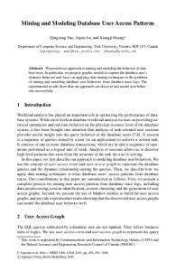
Moviegalaxies: The website http://moviegalaxies.com/ has assembled a large number of character networks based on movie scripts. There are over 800 networks available. Each network is weighted, although we discard the weights as we only use this for the model selection problem. Some of the properties of these networks are shown in Figure 1.

700

60

600

50

500

40

400 30

300 200

20

100

10

0 0

20

40 60 number of nodes

80

100

0

Fig. 1. Number of characters versus number of edges in the Moviegalaxies network data. The color shows how many graphs (according to the color bar) lie at the same (nodes, edges) bin.

6

3 3.1

Results Analysis of Novel Character Networks

Main characters from each of the novels analyzed scored consistently high in each of the six centrality measures. We present the centrality measures for the top twelve characters from the novel character networks in the figures below. Characters are ranked by increasing PageRank. For example, Harry, Ron and Hermione are identified as the top characters in Harry Potter and the Goblet of Fire. Further, our methods accurately predict the community structure for each of the three novels. Visualizations of the character networks and their community in the novels is found below. For Harry Potter and the Goblet of Fire the communities were: Hogwarts, the Dursleys, the Weasleys, Sytherin, and the inseparable friends Seamus and Dean. See Figure 2.

George Bill Charlie

Fred Lee Roberts

Molly

Seamus

Ginny

Percy Cho Crabbe

Maxime

Fleur

Dean Arthur

Hedwig

McGonagall

Neville

Goyle

Karkaroff

Pomfrey

Ludo

Lucius

Rita Fang

Bartemius

Hagrid

Viktor James

Draco

Albus Parvati

Cedric

Hermione

Sibyll

Voldemort

Ron

Cornelius Nick

Snape

Harry

Dobby

Frank

Colin

Dudley

Moody

Petunia Pigwidgeon

Winky

Sirius

Myrtle

Remus

Argus Amos

Bertha

Peeves

Crookshanks

Vernon Fawkes Lily

Wormtail

Fig. 2. The character network for Harry Potter and the Goblet of Fire. Each community is represented by a distinct color. The thickness of an edge is scaled to its weight, and the size of a name is scaled to the Pagerank score.

7

Fig. 3. Centrality measures for Harry Potter and the Goblet of Fire.

For Twilight, the three communities can be labeled as: vampires, high school students, and characters close to Charlie. See Figure 4.

Esme

Emmett

Rosalie

Alice James Snow

Carlisle Lee

Edward Varner

Angela

Jasper

Victoria

Laurent Cope

Eric

Jessica

Tyler

Phil

Jacob

Lauren

Mike

Banner

Bella Charlie

Billy Rene

Fig. 4. The character network for Twilight.

8

Fig. 5. Centrality measures for Twilight.

For The Stand, the government and the evil Las Vegas group emerged as separate communities. The free zone society was divided into three groups based on their relation to the main characters, Stu, Larry, and Nick. See Figure 6.

Peri

Olivia June

Kojak Julie

Charles

Mark Gina

Abagail

Nick

Glen

Patty

Harold Dick

Ralph Poke

Tom

Stu

Susan

Fran

Len

Larry

Kid

Barry

Lucy

Flagg

Starkey

Lloyd Hector

Nadine

Joe

Judge

Trashcan Dayna

Jenny Rita

BobbyTerry

Whitney

Rat-Man

Fig. 6. The character network for The Stand.

3.2

Model Selection Results

Hyperparameters for each classifier were selected using stratified, 5-fold cross validation. All features were normalized to have zero mean and unit variance before training. First, the random graph data was split into half training and half holdout. Classification performance

9

Fig. 7. Centrality measures for The Stand.

on the holdout set verified both the choice of hyperparameters and the separability of classes in our chosen feature space. All classifiers achieved nearly perfect classification on the holdout set, with over 0.98 precision and recall in nearly all cases (often exactly 1). The F1 score was at least 0.97. Thus, our four random graph models represent distinct classes. Table 2 shows model selection scores for the setup described in Section 2.2 (we train on the entire random graph data, and test on the original character network). These scores were calculated differently depending on the classifier. For the SVM algorithms, distance to the separating hyperplane was used. For AdaBoost, we use the final decision function, and soft decision probabilities were used for the random forests; see Figure 8. For all classifiers, a more positive (negative) score indicates more confidence the original graph does (not) belong to the model. Clearly, CL is the best random graph model for all three novels, with each remaining model taking a distant second place in at least one case. Figure 9 shows our naming convention for the motifs used in our graph profile features. The most important features for the CL SVM hyperplanes were predominantly cliques: induced subgraphs H3 , F5 , F9 , and F10 . For the tree-based classifiers, the most important motifs for distinguishing among graph models include some disconnected subgraphs: H0 , H2 , F2 , F5 , and F10 . The eigenvalue histograms generally had low importance for all machine learning classifiers. Thus, similar results were obtained using only graph profile features. See Table 3. Figure 10 shows similar aggregate results for the 800 character networks in the Moviegalaxies data set, with CL as the best random graph model for the overwhelming number of character networks.

4

Discussion and Future Work

We presented a comparative and quantitative analysis of character networks arising from various novels and films. In particular, we analyzed the weighted social networks from the

10 Table 2. Model selection scores for random graph models using graph profiles and eigenvalue histograms as features. CL is selected by all machine learning classifiers as the best model.

Novel Goblet

Twilight

The Stand

Classifier SVM-`2 SVM-`1 Forest AdaBoost SVM-`2 SVM-`1 Forest AdaBoost SVM-`2 SVM-`1 Forest AdaBoost

PA 2.78 −0.66 0.00 −47.2 −0.671 −3.08 0.00083 −43.06 −1.52 −2.32 0.00 −47.04

CL 4.59 3.81 0.91 47.4 4.49 5.19 0.800 32.30 2.65 2.87 0.946 50.03

ER −1.10 −1.55 0.094 25.5 −2.98 −2.06 0.0248 10.74 −1.24 −1.14 0.00 37.83

CFG −10.65 −10.80 0.0011 −25.7 −9.39 −12.21 0.175 0.0205 −3.87 −4.97 0.0544 −40.82

Table 3. Model selection scores for random graph models using graph profiles alone as features. Once again, CL is selected by all machine learning classifiers as the best model.

Novel Goblet

Twilight

The Stand

Classifier SVM-`2 SVM-`1 Forest AdaBoost SVM-`2 SVM-`1 Forest AdaBoost SVM-`2 SVM-`1 Forest AdaBoost

PA 3.18 −0.68 0.000 −47.2 −0.54 −2.78 0.00 −39.72 −1.18 −2.35 0.00 −46.49

CL 4.44 3.81 0.998 47.4 5.51 5.25 1.00 34.51 2.58 2.86 0.94 50.32

ER −1.15 −1.53 0.002 25.5 −2.73 −2.02 0.00 −7.44 −1.33 −1.14 0.00 38.36

CFG −10.64 −10.81 0.000 −25.7 −9.52 −12.24 0.00 12.66 −4.02 −4.99 0.06 −42.19

H_2