MINING BALANCED PATTERNS IN WEB ACCESS DATA Edgar H. de Graaf, Joost N. Kok and Walter A. Kosters Leiden Institute of Advanced Computer Science Leiden University Leiden, The Netherlands email:
[email protected] ABSTRACT In web access analysis of a large-scale website the behaviour of visitors accessing the website is examined. An example instance of a pattern is if a visitor accesses the same parts of the website every seven days; we will call such types of patterns balanced patterns. We define balanced patterns using standard deviation and average. We propose a new approach for pruning such patterns. In comparison with related work the required algorithm and definitions will be relatively simple. Furthermore, the new pruning threshold is intuitive from an analysts perspective. KEY WORDS Support Measures, Data Mining, Frequent Pattern Mining, Web Access Data
1 Introduction Mining frequent patterns is an important area of data mining, where we discover substructures that occur often in (semi-)structured data. In this work we will further investigate one of the simplest (and most researched) structures: itemsets. Our datasets can be seen as a sequence of transactions arriving in order, where each transaction is an itemset. However the algorithm and definitions that we introduce are easily extended to sequential pattern mining, tree and graph mining. We consider web access data: a transaction is then a set of accessed webpages during a small session. The analysis of online visitor behavior is becoming an increasingly more popular area of research, as shown for example by the development of the Urchin Traffic Monitor by Google (see [1]). In our analysis of web access data we are interested in the behaviour of visitors of the website. We will look for repeated occurrence of patterns (subsets) in the sequence of transactions (itemsets) such that the lengths of the gaps between the occurrences are similar. To this end, this paper makes the following contributions: — We will define balanced patterns and show how to use them: these balanced patterns will enable the analyst to better filter uninteresting patterns (Section 2). — Furthermore we will propose an algorithm for mining balanced patterns (Section 3). — Finally we will empirically show that the algorithm
can find interesting patterns efficiently in real world data, e.g., web access data (Section 4). One of the main differences with sequential pattern mining is that our dataset consists of just one sequence of transactions. In Section 2.1 we will recall some definitions [2] on the subject of mining regular occurring patterns. In Section 2.2 we will define our current approach where we introduce balanced patterns. This research is related to work done on the (re)definition of support, using time with patterns and the incorporation of distance measured by the number of transactions between pattern occurrences. The notion of support was first introduced by Agrawal et al. in [3] in 1993. Since then many new and faster algorithms where proposed. We make use of E CLAT, the algorithm developed by Zaki et al. in [4]. Steinbach et al. in [5] generalized the notion of support providing a framework for different definitions of support in the future. Our work is also related to work described in [6] where association rules are mined that only occur within a certain time interval. In other work time series data is mined for periodic patterns [7]. Here the dataset consists of sequences representing, e.g., one day where each item represents a value changing as the day goes by. Time series data is a related issue but different since our method aims to discover itemsets occurring with a transaction wise regular interval. Furthermore there is some minor relation with mining data streams as described in [8, 9, 10], in the sense that they use time to say something about the importance of a pattern. Finally this work is related to some of our earlier work. Results from [11] indicated that the biological problem could profit from incorporating consecutiveness into frequent itemset mining, which was elaborated in [12]. In the case of regular occurring patterns we also make use of the transactions and the distance between them.
2 Regular Occurrence In this section we will first repeat the definition of stable patterns to better understand the problems and the difference with the definition of balanced patterns. Roughly speaking, patterns that occur at regular intervals (e.g., at equidistant time stamps) will be called stable or balanced. In the case of stable patterns, in order to judge this prop-
erty, we will determine how often events occur “in the middle” between two other events [2]. In the case of balanced patterns we prune patterns that do not have at least one frequent intermediate distance (between all occurrences) and we filter those patterns that have a too high deviation for all distances between successive occurrences. Furthermore we filter patterns that do not reach a certain minimal average distance for all successive occurrences. 2.1 Stable Patterns In this paper a dataset consists of transactions that take zero time. Each transaction is an itemset, i.e., a subset of {1, 2, 3, . . . , max } for some fixed integer max . The transactions can have time stamps; if so, we assume that the transactions take place at different moments. We choose some notion of distance between transactions; examples include: (1) the distance is the time between the two transactions and (2) the distance is the number of transactions (in the original dataset) strictly in between the two transactions. In the case of (2) transactions should arrive at a constant rate for not having skewed results. In this paper we will use (2) in all our examples, since the transactions in the datasets are uninterrupted arriving at a constant rate. This enables the algorithm to decide the time between two pattern occurrences without the need to compare timestamps. We will define Trans(p) as the series of transactions that contain pattern (i.e., itemset) p; the support of a pattern p is the number of elements in this ordered series. We now define w-stable patterns as itemsets that occur frequent (support ≥ minsup) in the dataset and that have stability value ≥ minstable, where the values minsup and minstable are user-defined thresholds. A wgood triple (L, M, R) consists of three transactions L, M and R, occurring in this order, such that |distance(L, M )− distance(M, R)| ≤ 2 · w; here w is a pregiven small constant ≥ 0, e.g., w = 0. The stability value of a pattern p is the number of w-good triples in Trans(p), plus the number of transactions in Trans(p) that occur as left endpoint in a w-good triple, plus the number of transactions in Trans(p) that occur as right endpoint in a w-good triple. Note that the stability value of a pattern p′ with p′ ⊆ p is at least equal to that of p: the so-called A PRIORI or anti-monotone property. Also note that the stability value remains the same if we consider the dataset in reverse order. In our work on stable patterns [2] we showed that equidistant events are “very” stable (in case w = 0). Example 1 Suppose we have the following itemsets in our dataset: transaction 1: {A, B, C} transaction 2: {D, C} transaction 3: {A, B, E} transaction 4: {E, F } transaction 5: {A, B, F } transaction 6: {E, F }
transaction 7: {A, B, F } transaction 8: {E, F } transaction 9: {A, B, C} The stability value (with w = 0) of {A,B} is 4+3+3 = 10, the maximal value possible. Indeed, there are 4 0-good triples; we have 3 transactions that are left (right) endpoint of a 0-good triple (see picture below, left). If we insert two transactions {E, F } between transaction 1 and 2, and also two between 8 and 9, we still have 4 0-good triples, but now we only have 2 transactions that are left (right) endpoint of a good 0-triple (see picture below, right), leading to stability value 4 + 2 + 2 = 8 < 10. By the way, this example also shows that in order to guarantee equidistance one has to add left and right endpoints to the stability value. s
s
s
s
s
s
s
s
s
s
2.2 Balanced Patterns In this section we will define balanced patterns. We first discuss several problems and possibilities, and finally give the proper definition. We call the occurrences balanced if between two successive occurrences there is (almost) always the same amount of transactions. The problem with patterns with balanced occurrences is that an itemset may occur less balanced than a superset of this itemset. Patterns occurring with a balanced interval do not have the anti-monotone property, where the subset is either equally good or better than the superset. However first we notice that for the distance between all occurrences the count for one distance can only decrease for a superset. Example 2 Say that item A occurs in transactions 1, 3, 4, 7 and 10 and item B occurs in transaction 4, 7, 10 and 13, then the itemset {A, B} will occur in transaction 4, 7 and 10. Both A and B have three times two transactions between (successive and non-successive) occurrences. For instance, the non-successive occurrences 1 and 4 of A have the two transactions 2 and 3 in-between. However, the itemset {A, B} has only two times two transactions between occurrences, because an occurrence can only become a nonoccurrence and not the other way around. For our definition of balanced patterns we first notice that all balanced occurrences (successive and nonsuccessive) should have at least one intermediate distance a minimal number of times. Furthermore if you count the distances between all occurrences then this count is antimonotone: a superset never has more of one particular distance. This is obvious because the number of occurrences will never increase for a superset and as a consequence the count of one particular distance will never increase. This property is also anti-monotone if we limit the distances we count, e.g., we count a distance only if it is smaller than 10 in-between transactions. Example 3 The following table, where we only count up to 4 in-between transactions, is an example:
In-between transactions Count
0 0
1 5
2 200
3 30
4 199
The balanced value for the pattern with these counts will be 200, the highest count in the table. Still if we only look at the distance count we will not find the balanced patterns we want, since patterns that occur with very unbalanced intervals might still have a minimum amount of one particular distance. We filter those patterns by keeping the distance between occurrences that immediately succeed each other (instead of taking all distances). If a pattern is balanced then these distances should approach the average of all these distances. Their standard deviation will be near 0, since one distance should occur the most. Note that in calculating the standard deviation we do not limit the distances we consider. This can be done because the number of possible distances is far less for successive occurrences. Now we can find all balanced patterns, however we will still find many patterns that are occurring every transaction. Their distance is almost always 0 and although they are well balanced they are often not interesting. These patterns can be filtered if we demand a certain average distance, e.g., if the user-defined threshold minavg is set to 1 then all these patterns will be filtered out, since their average distance approaches 0. Before we define balanced patterns, we first introduce the so-called O-series. This series simply indicates in which transactions from the original database a given itemset occurs: Definition 1 (O-series) Suppose we have an itemset I and let Oj ∈ {0, 1} (j = 1, 2, . . . , r) denote whether or not the j th transaction in some ordered subset S of the database D contains I (Oj is 1 if it does contain I, and 0 otherwise; the series of Oj ’s are referred to as the O-series), r = |S|. The function ϕ : N → N is a translation from the index j for the j-th transaction in S to the index ϕ(j) giving the position of this same transaction in D. This O-series is used in the definition of balanced patterns. We will introduce three parameters, minnumber, maxstdev and minavg: Definition 2 (Balanced Pattern) An itemset I is called a balanced pattern if among all occurrence pairs Oi = 1 and Oj = 1, where i < j, at least one distance (= j − i − 1) occurs at least a user-defined number minnumber of times. Also the standard deviation σ for all distances between successive occurrences is at most equal to a userdefined value maxstdev. Two occurrences Oi and Oj are successive if Oi = 1 and Oj = 1 and there is no k, i < k < j, where Ok = 1. Finally the mean µ for all distances between successive occurrences is at least equal to a userdefined value minavg. The three parameters of Definition 2 are more intuitive and easier to estimate in comparison to the stability value as defined in the previous section. Moreover, stability
value is more sensitive to small variations in the occurrence interval.
3 Algorithm We now consider algorithms that find all frequent itemsets, given a database. A frequent itemset is an itemset with support at least equal to some pre-given threshold, the socalled minsup. Thanks to the A PRIORI property many efficient algorithms exist. However, the really fast ones rely upon the concept of FP- TREE or something similar, which does not keep track of in-between distances. This makes these algorithms hard to adapt for use in balanced patterns. One fast algorithm that does not make use of FPTREE s is called E CLAT [4]. E CLAT grows patterns recursively while remembering which transactions contained the pattern, making it very suitable for balanced patterns. In the next recursive step only these transactions are considered when counting the occurrence of a pattern. All counting is done by using a matrix and patterns are extended with new items using the order in the matrix. This can easily be adapted to incorporate balance counting. Our algorithm BALANCE C LAT will use the E CLAT algorithm. However instead of counting support we count the different distances between all occurrences, e.g., pattern A has 10 times 3 transactions between occurrences. We will prune on this value instead of pruning on the minimal support threshold. In this case the user-defined threshold will be the minimal number of times at least one of ℓ + 1 distances {0, 1, 2, . . . , ℓ} is seen. For balanced patterns we consider this threshold to be the minnumber threshold. As said before, we can only find balanced patterns if we also demand a maximal standard deviation for distances between occurrences. This will be done by introducing the maxstdev threshold. Usually we are not interested in patterns occurring in every transaction. We introduce a third user-defined threshold that demands a minimal average distance: minavg. For maxstdev and minavg we only use distances between successive occurrences and for minnumber all distances ≤ ℓ. The main adaptation to E CLAT is replacing support with a balance value denoted with t. Also the algorithm calculates the standard deviation (stdev ) and average distance (avgdist ) for the successive occurrences. The standard deviation for succdists can simply be calculated in the following way: sP
− i)2 · succdists i i succdists i
i (avg (succdists) P
(1)
E CLAT can now prune using the balance value t (if t < minnumber) and patterns are only displayed if their standard deviation and average distance are sufficient. These straightforward adaptations are not given in detail. Standard deviation changes if patterns occur less balanced in a certain small number of successive transac-
j := 2, h := −1 succdists := array of distance counts between successive occurrences alldists := array of distance counts (≤ ℓ) between all occurrences while ( j ≤ r ) do if ( Oj = 1 ) then i := 1 while ( i < j ) do if ( Oi = 1 and ϕ(j) − ϕ(i) − 1 ≤ ℓ ) then alldists[ϕ(j) − ϕ(i) − 1]++ fi i++ od if ( h 6= −1 ) then succdists[ϕ(j) − ϕ(h) − 1]++ fi h := j fi j ++ od t := max (alldists), the largest count in the sequence stdev := standard deviation for succdists avgdist := average for succdists, also denoted with avg(succdists)
tions, small periods. In some cases it might be preferable to remove the influence of these periods. One possible approach is to calculate average distance and the standard deviation for frequent distances (for successive occurrence) only. The value for filtering with standard deviation for the sequences Q = hy|y = succdisti , y ≥ mindfreqi and I = hi|y = succdisti , y ≥ mindfreqi will be:
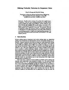
First the BALANCE C LAT algorithm is executed with maxstdev = 2.5, minavg = 2.0 and minnumber = 150. Figure 1 displays the number of expected patterns that were actually found by the algorithm. We see that the algorithm detects most patterns up to a noise level of 15%. Due to the way we generate noise, long patterns become less likely as the noise level increases. With a high noise level we only find the patterns of 1 item in length. This can be improved if we change our settings for maxstdev and minavg, but we kept them fixed for comparison reasons.
if Q is not empty 35
otherwise
(2) Note that via the threshold mindfreq the user decides when a distance is considered frequent.
4 Results and Performance
30
25 Nr. of Expected Patterns
rP 2 i (avg(Q) P − Ii ) · Qi stdev = Q i i maxstdev + 1
called find-noise-x% where x is a noise value ranging from 0 to 30. E.g., if the noise is 10%, this means there is a 10% chance that one element of the balanced pattern does not occur when it “should”. In each of these find-noise-x% datasets one pattern of 5 of the 200 items occurs every 4 transactions (so distance = 3) and each dataset has 2,000 transactions. Furthermore the remaining items have a probability of 50% to occur. If 5Pitems always occur balanced 5 like this, we expect to find k=1 5!/(5 − k)!k! = 31 patterns when we would apply standard frequent itemset mining algorithms. We will call these frequent occurring itemsets expected patterns. The first real dataset we test our algorithm on is called the website dataset. This dataset is based on an access log of the website of the Computer Science department of Leiden University, as said before. It contains all 1,991 items of the web-pages that were visited, grouped in half-hour blocks, so each of the 1,488 transactions contains the pages visited during one half-hour. The second real dataset is called the one-visitor dataset and it stores the webpages accessed by one heavy user of the former PortalExecutivo.com website. Each day represents one transaction of pages accessed. Some days there is no access and some of the 1,603 transactions are empty. Webpages are categorised resulting in a total of 185 possible items for every transaction.
20
15
10
5
The experiments were done for three main reasons. First of all we want to show that known balanced patterns will be found also in the case of noise. Secondly we want to show that interesting balanced patterns can be found in real datasets. Finally we will discuss runtime for real data and how the minnumber threshold influences runtime. Our implementation of the balanced pattern mining algorithm is called BALANCE C LAT. All experiments were performed on an Intel Pentium 4 64-bits 3.2 GHz machine with 3 GB memory. As operating system Debian Linux 64bits was used with kernel 2.6.8-12-em64t-p4. The synthetic datasets used in our first experiment are
0 0
5
10
15 Noise Level (0%-30%)
20
25
30
Figure 1. The effect of noise on the algorithm using the find-noise-x% datasets. We can use the mindfreq threshold to decrease the influence of small noisy periods on the balanced occurrences. Figure 2 shows how the effect of noise becomes less if we set a mindfreq of 50. Now one also finds more of the other patterns that happen to occur reasonably balanced, however we can filter them by lowering maxstdev .
35
80000
70000
30
60000
Avg. Runtime (ms)
Nr. of Expected Patterns
25
20
15
50000
40000
30000
10 20000 5
10000
0
0 5
10
15 Noise Level (0%-30%)
20
25
30
Figure 2. The effect of noise on the algorithm using the find-noise-x% datasets with mindfreq = 50. With our next experiment we want to show the effect of dataset size on the algorithm, scalability. To this end we measured runtime for different sizes of the dataset where each transaction can contain up to 200 items and 5 items occur every 4 transactions and the remaining items have a probability 50% to occur, the find-noise-0% dataset. In Figure 3 first the runtime drops; this is because many patterns have distances occurring only a few times. E.g., when the dataset size is 100 then minnumber = 0.1 · 100 = 10. Many patterns have distances that occur at least 10 times. As this effect becomes less, runtime increases and eventually it becomes nearly linear. 11000
50
100
150
200 250 The minnumber threshold
300
350
400
Figure 4. Runtime in ms for different values of minnumber for the website dataset (maxstdev = 1.0, minavg = 2.0, ℓ = 10). 500
450
400
350 Avg. Runtime (ms)
0
300
250
200
150
100
50 0
5
10
15 The minnumber threshold
20
25
30
Figure 5. Runtime in ms for different values of minnumber for the one-visitor dataset (maxstdev = 5.0, minavg = 2.0, ℓ = 10).
10000
9000
2
7000
6000
5000
4000
3000
2000 0
2
4
6
8 10 12 Nr. of Transaction x 100
14
16
18
20
Figure 3. Runtime in ms for different dataset sizes for the find-noise-0% dataset; minnumber is 10% of the dataset size (maxstdev = 1.0, minavg = 2.0, ℓ = 10). Figure 4 shows how the runtime for the website dataset drops fast as minnumber increases. Figure 5 also shows a drop of runtime for the one-visitor dataset. Many patterns in the one-visitor dataset occur mostly unstable and only some occur stable in such a way that the standard deviation of the interval does not suffer too much (becomes more than minavg ). One pattern that was found was the access of research and training part of the website on the same day every seven days, see Figure 6. Also this pattern lasted for more than one month. Another example is given below, showing the count for distances between successive occurrences. This pattern shows that the websites of two cooperating professors are accessed every half-hour and often at least every hour.
1 = transaction contains pattern, 0 = otherwise
Avg. Runtime (ms)
8000
1.5
1
0.5
0 600
605
610
615
620
625
630
Transactions
Figure 6. The occurrence of one pattern discovered with BALANCE C LAT in the one-visitor dataset (minnumber = 20, maxstdev = 3.0, minavg = 1.5, ℓ = 7). Example 4 The distances (with count ≥ 20) between successive occurrences and their counts for one pattern (two professors & the main page) in the website dataset (maxstdev = 2.0, minavg = 1.0, ℓ = 10): In-between transactions Count
0 385
1 171
2 78
3 25
4 23
Finally we also applied the BALANCE C LAT algorithm to the Nakao dataset used in [12]. In this dataset each of the 2,124 transactions is in fact a clone located on the human chromosomes. The items are the patients with a higher
than normal value for this clone (≥ 0.225). The specifics of the dataset can be found in [13]. The parameter minavg was set to 0.0, because the interesting patterns are expected to occur very close to each other. Also mindfreq = 10 because patterns were expected to have small periods of transactions where they occurred unbalanced. Furthermore maxstdev = 0.2, ℓ = 10 and minnumber = 100. Results were similar to results found with consecutive support as presented in [12] where most consecutive patterns occurred close together in chromosome 9, see Figure 7. However, the difference with consecutive support is that it looks at all gap sizes between occurrences and it does not have to maintain a count for all possible distances. 20
Imielinski and R. Srikant, Minrules between sets of items in Proc. ACM SIGMOD Conference of Data, Washington, D.C., USA,
[4] M. Zaki, S. Parthasarathy, M. Ogihara and W. Li, New algorithms for fast discovery of association rules, Proc. 3th Int. Conference on Knowledge Discovery and Data Mining, Newport Beach, USA, 1997, 283–296. [5] M. Steinbach, P. Tan, H. Xiong and V. Kumar, Generalizing the notion of support, Proc. 10th Int. Conference on Knowledge Discovery and Data Mining, Seattle, USA, 2004, 689–694. [6] Y. Li, P. Ning, X.S. Wang and S. Jajodia, Discovering calendar-based temporal association rules, Proc. 8th Int. Symposium on Temporal Representation and Reasoning, Cividale del Friuli, Italy, 2001, 111–118.
15
# Patterns
[3] R. Agrawal, T. ing association large databases, on Management 1993, 207–216.
10
5
0 0
500
1000
1500
2000
2500
Clone
Figure 7. The occurrence of one pattern discovered with BALANCE C LAT in the Nakao dataset (minnumber = 20, maxstdev = 0.2, minavg = 0.0, mindfreq = 10, ℓ = 10).
5 Conclusions We have presented a new way of mining for patterns occurring with a regular interval. In comparison with previous methods we now use a pruning threshold minnumber that is more intuitive to website analysts and easier to estimate. Definitions and algorithm are less complex and easier to understand. The analyst only indicates the number of times at least one intermediate distance should occur. Such a distance is the number of transactions between two occurrences of the pattern, since transactions arrive uninterrupted at a constant rate. One can also use time stamps to calculate the time between occurrences. In this work we call patterns with a regular interval balanced and we discuss an algorithm to find them efficiently. Runtime performance and scalability are evaluated through experiments. In the future we plan to study balanced patterns with more complicated intermediate intervals. Also research will be done on effectively visualizing balanced patterns.
References [1] Google Urchin, http://www.google.com/support/urchin45/. [2] E.H. de Graaf and W.A. Kosters, Mining for stable patterns: Regular intervals between occurrences, 18th Belgium-Netherlands Conference on Artificial Intelligence, Namur, Belgium, 2006, 149–155.
[7] J. Yang, W. Wang and P.S. Yu, Mining asynchronous periodic patterns in time series data, IEEE Transactions on Knowledge and Data Engineering, 15(3), 2003, 613–628. [8] Y. Chen, G. Dong, J. Han, B. Wah and J. Wang, Multidimensional regression analysis of time-series data streams, Proc. 28th Int. Conference on Very Large Data Bases, Hong Kong, China, 2002, 323–334. [9] C. Giannella, J. Han, J. Pei, X. Yan and P. Yu, Mining frequent patterns in data streams at multiple time granularities, Proc. NSF Workshop on Next Generation Data Mining, Baltimore, USA, 2002, 191–210. [10] W. Teng, M. Chen and P.S. Yu, A regression-based temporal pattern mining scheme for data streams, Proc. 29th Int. Conference on Very Large Data Bases, Berlin, Germany, 2003, 93–104. [11] J.M. de Graaf, R.X. de Menezes, J.M. Boer and W.A. Kosters, Frequent itemsets for genomic profiling, Proc. First International Symposium on Computational Life Sciences, Konstanz, Germany, 2005, 104–116. [12] E.H. de Graaf, J.M. de Graaf and W.A. Kosters, Using consecutive support for genomic profiling, Proc. ECML/PKDD Workshop on Data and Text Mining for Integrative Biology, Berlin, Germany, 2006, 16– 27. [13] K. Nakao, K.R. Mehta, J. Fridlyand, D.H. Moore, A.N. Jain, A. Lafuente, J.W. Wiencke, J.P. Terdiman and F.M. Waldman, High-resolution analysis of DNA copy number alterations in colorectal cancer by array-based comparative genomic hybridization, Carcinogenesis, 25, 2004, 1345–1357.