Mining Fuzzy Multidimensional Association Rules ... - Petra's Repository

(IJCNS) International Journal of Computer and Network Security, Vol. 1, No. 2, November 2009

60

Mining Fuzzy Multidimensional Association Rules Using Fuzzy Decision Tree Induction Approach* Rolly Intan1、 Oviliani Yenty Yuliana2, Andreas Handojo3 Department of Informatics Engineering, Petra Christian University, Siwalankerto 121-131, Surabaya 60236, Indonesia 1 [email protected], [email protected], [email protected]

Abstract: Mining fuzzy multidimensional association rules is one of the important processes in data mining application. This paper extends the concept of Decision Tree Induction (DTI) dealing with fuzzy value in order to express human knowledge for mining fuzzy multidimensional association rules. Decision Tree Induction (DTI), one of the Data Mining classification methods, is used in this research for predictive problem solving in analyzing patient medical track records. Meaningful fuzzy labels (using fuzzy sets) can be defined for each domain data. For example, fuzzy labels poor disease, moderate disease, and severe disease are defined to describe a condition/type of disease. We extend and propose a concept of fuzzy information gain to employ the highest information gain for splitting a node. In the process of generating fuzzy multidimensional association rules, we propose some fuzzy measures to calculate their support, confidence and correlation. The designed application gives a significant contribution to assist decision maker for analyzing and anticipating disease epidemic in a certain area.

Keywords: Data Mining, Classification, Decision Tree Induction, Fuzzy Set, Fuzzy Association Rules.

1. Introduction Decision Tree Induction (DTI) has been used in machine learning and in data mining as a model for prediction a target value based on a given relational database. There are some commercial decision tree applications, such as the application for analyzing a return payment of a loan for owning or renting a house [16] and the application of software quality classification based on the program modules risk [17]. Both applications inspire this research to develop an application for analyzing patient medical track record. The Application is able to present relation among (single/group) values of patient attribute in decision tree diagram. In the developed application, some domains of data need to be utilized by meaningful fuzzy labels. For example, fuzzy labels poor disease, moderate disease, and severe disease describe a condition/type of disease; young, middle aged and old are used as the fuzzy labels of ages. Here, a fuzzy set is defined to express a meaningful fuzzy label. In order to utilize the meaningful fuzzy labels, we need to extend the concept of (crisp) DTI using fuzzy approach. Simply, the extended concept is called Fuzzy Decision Tree (FDT). To generate FDT from a normalized database that consists of several tables, there are several sequential processes as shown in Figure 1. First is the process of joining tables known as Denormalization of

Database as discussed in [4]. The process of denormalization can be provided based on the relation of tables as presented in Entity Relationship Diagram (ERD) of a relational database. Result of this process is a general (denormalized) table. Second is the process of constructing FDT generated from the denormalized table.

Figure 1. Process of mining association rules In the process of constructing FDT, we propose a method how to calculate fuzzy information gain by extending the existed concept of (crisp) information gain to employ the highest information gain for splitting a node. The last is the process of mining fuzzy association rules. In this process, fuzzy association rules are mined from FDT. In the process of mining fuzzy association rules, we propose some fuzzy measures to calculate their support, confidence and correlation. Minimum support, confidence and correlation can be given to reduce the number of mining fuzzy association rules. The designed application gives a significant contribution to assist decision maker for analyzing and anticipating disease epidemic in a certain area. The structure of the paper is the following. Section 2 discusses denormalized process of data. Section 3 gives a basic concept of association rules. Definition and formulation of some measures such as support, correlation and confidence rule as used for determining interestingness of the association rules are briefly recalled. Section 4, as main contribution of this paper is devoted to propose the concept and algorithm for generating FDT. Section 5 proposes some equations of fuzzy measures that play important role in the process of mining fuzzy multidimensional association rules. Section 6 demonstrates the algorithm and in a simple illustrative results. Finally a conclusion is given in Section 7.

(IJCNS) International Journal of Computer and Network Security, 61 Vol. 1, No. 2, November 2009

2. Denormalization Data In general, the process of mining data for discovering association rules has to be started from a single table (relation) as a source of data representing relation among item data. Formally, a relational data table [13] R consists of a set of tuples, where ti represents the i-th tuple and if there are n domain attributes D, then ti = ( d i1 , d i 2 , L , d in ). Here, dij is an atomic value of tuple ti with the restriction to the domain Dj, where d ij ∈ D j . Formally, a relational data table R is defined as a subset of the set of cross product D1 × D2 ×L× Dn , where D = {D1 , D2 , L, Dn } . Tuple

Figure 2. Example of ERD Physical Design

t (with respect to R) is an element of R. In general, R can be shown in Table 1.

From the example, it is clearly seen that there are four tables: A, B, C and D. Here, all tables are assumed to be independent for they have their own primary keys. Cardinality of relationship between Table A and C is supposed to be one to many relationships. It is similar to relationship between Table A and B as well as Table B and D. Table A consists of four domains/fields, D1, D2, D3 and D4; Table B also consists of four domains/fields, D1, D5, D6 and D7; Table C consists of three domains/fields, D1, D8 and D9; Table D consists of four domains/fields, D10, D11, D12 and D5. Therefore, there are totally 12 domains data as given by D={D1, D2, D3, …, D11, D12}. Relationship between A and B is conducted by domain D1. Table A and C is also connected by domain D1. On the other hand, relationship between B and D is conducted by D5. Relation among A, B, C and D can be also represented by graph as shown in Figure 3.

Table 1: A Schema of Relational Data Table

Tuples D1 D2 L Dn t1 d11 d12 L d1n t2 M

d21 d22 L d2n M M O M

tr

dr1 dr2 L drn

A normalized database is assumed as a result of a process of normalization data in a certain contextual data. The database may consist of several relational data tables in which they have relation one to each others. Their relation may be represented by Entities Relationship Diagram (ERD). Hence, suppose we need to process some domains (columns) data that are parts of different relational data tables, all of the involved tables have to be combined (joined) together providing a general data table. Since the process of joining tables is an opposite process of normalization data by which the result of general data table is not a normalized table, simply the process is called Denormalization, and the general table is then called denormalized table. In the process of denormalization, it is not necessary that all domains (fields) of the all combined tables have to be included in the targeting table. Instead, the targeting denormalized table only consists of interesting domains data that are needed in the process of mining rules. The process of denormalization can be performed based on two kinds of data relation as follows. 2.1. Metadata of the Normalized Database Information of relational tables can be stored in a metadata. Simply, a metadata can be stored and represented by a table. Metadata can be constructed using the information of relational data as given in Entity Relationship Diagram (ERD). For instance, given a symbolic ERD physical design is arbitrarily shown in Figure 2.

{D1}

C

{D1}

A

{D5}

B

D

Figure 3. Graph Relation of Entities

Metadata expressing relation among four tables as given in the example can be simply seen in Table 2.

Table-1 Table A Table A Table B

Table 2: Example of Metadata Table-2 Relations {D1} Table B {D1} Table C {D5} Table D

Through the metadata as given in the example, we may construct six possibilities of denormalized table as shown in Table 3. Table 3: Possibilities of Denormalized Tables No. Denormalized Table 1 CA(D1,D2,D3,D4,D8,D9); CA(D1,D2,D8,D9); CA(D1,D3,D4,D9), etc. 2 CAB(D1,D2,D3,D4,D8,D9,D5,D6,D7), CAB(D1,D2,D4,D9,D5,D7), etc. 3 CABD(D1,D2,D3,D4,D5,D6,D7,D8,D9, D10,D11,D12), etc. 4 AB(D1,D2,D3,D4,D5,D6,D7), etc. 5 ABD(D1,D2,D3,D4,D5,D6,D7,D10, D11,D12), etc. 6 BD(D5,D6,D7,D10,D11,D12), etc.


62

CA(D1,D2,D3,D4,D8,D9) means that Table A and C are joined together, and all their domains are participated as a result of joining process. It is not necessary to take all domains from all joined tables to be included in the result, e.g. CA(D1,D2,D8,D9), CAB(D1,D2,D4,D9,D5,D7) and so on. In this case, what domains included as a result of the process depends on what domains are needed in the process of mining rules. For D1, D8 and D5 are primary key of Table A. C and B, they are mandatory included in the result, Table CAB. 2.2. Table and Function Relation It is possible for user to define a mathematical function (or table) relation for connecting two or more domains from two different tables in order to perform a relationship between their entities. Generally, the data relationship function performs a mapping process from one or more domains from an entity to one or more domains from its partner entity. Hence, considering the number of domains involved in the process of mapping, it can be verified that there are four possibility relations of mapping. Let A( A1 , A2 , L , An ) and B ( B1 , B2 ,L, Bm ) be two different entities (tables). Four possibilities of function f performing a mapping process are given by: o One to one relationship

f : Ai → Bk o

One to many relationship

f : Ai → B p1 × B p2 × L × B pk o

Many to one relationship

f : Ar1 × Ar2 × L× Ark → Bk o

Many to many relationship f : Ar1 × Ar2 × L × Ark → B p1 × B p2 × L × B pk

Obviously, there is no any requirement considering type and size of data between domains in A and domains in B. All connections, types and sizes of data are absolutely dependent on function f. Construction of denormalization data is then performed based on the defined function.

3. Fuzzy Multidimensional Association Rules Association rule finds interesting association or correlation relationship among a large data set of items [1,10]. The discovery of interesting association rules can help in decision making process. Association rule mining that implies a single predicate is referred as a single dimensional or intradimension association rule since it contains a single distinct predicate with multiple occurrences (the predicate occurs more than once within the rule). The terminology of single dimensional or intradimension association rule is used in multidimensional database by assuming each distinct predicate in the rule as a dimension [1]. Here, the method of market basket analysis can be extended and used for analyzing any context of database. For instance, database of medical track record patients is analyzed for finding association (correlation) among diseases taken from the data of complicated several diseases suffered by patients in a certain time. For example, it might be discovered a Boolean association rule “Bronchitis

⇒ Lung

Cancer” representing relation between “Bronchitis” and “Lung Cancer” which can also be written as a single dimensional association rule as follows: Rule-1 Dis ( X , " Bronchitis " ) ⇒ Dis ( X , " Lung Cancer" ),

where Dis is a given predicate and X is a variable representing patient who have a kind of disease (i.e. “Bronchitis” and “Lung Cancer”). In general, “Lung Cancer” and “Bronchitis” are two different data that are taken from a certain data attribute, called item. In general, Apriori [1,10] is used an influential algorithm for mining frequent itemsets for mining Boolean (single dimensional) association rules. Additional related information regarding the identity of patients, such as age, occupation, sex, address, blood type, etc., may also have a correlation to the illness of patients. Considering each data attribute as a predicate, it can therefore be interesting to mine association rules containing multiple predicates, such as: Rule-2: Age( X , "60") ∧ Smk( X , " yes" ) ⇒ Dis( X , " Lung Cancer"), where there are three predicates, namely Age, Smk (smoking) and Dis (disease). Association rules that involve two or more dimensions or predicates can be referred to as multidimensional association rules. Multidimensional association rules with no repeated predicate as given by Rule-2, are called interdimension association rules [1]. It may be interesting to mine multidimensional association rules with repeated predicates. These rules are called hybriddimension association rules, e.g.: Rule-3: Age( X , "60" ) ∧ Smk ( X , " yes" ) ∧ Dis( X , " Bronchitis " ) ⇒ Dis( X , " Lung Cancer" ), To provide a more meaningful association rule, it is necessary to utilize fuzzy sets over a given database attribute called fuzzy association rule as discussed in [4,5]. Formally, given a crisp domain D, any arbitrary fuzzy set (say, fuzzy set A) is defined by a membership function of the form [2,8]:

A : D → [0,1].

(1)

A fuzzy set may be represented by a meaningful fuzzy label. For example, “young”, “middle-aged” and “old” are fuzzy sets over age that is defined on the interval [0, 100] as arbitrarily given by[2]:


support ( A ⇒ B ) = support( A ∪ B ) # tuples ( A and B) = , # tuples (all _ data )

, x ≤ 20 1  young ( x ) = ( 35 − x ) / 15 , 20 < x < 35 0 , x ≥ 35  , x ≤ 20 or x ≥ 60 0 . ( x − 20 ) / 15 , 20 < x < 35  middle _ aged ( x ) =  ( 60 − x ) / 15 , 45 < x < 60 1 , 35 ≤ x ≤ 45 0  old ( x ) = ( x − 45 ) / 15 1 

where #tuples(all_data) is the number of all tuples in the relevant data tuples (or transactions). For example, a support 30% for the association rule (e.g., Rule-1) means that 30% of all patients in the all data medical records are infected both bronchitis and lung cancer. From (3), it can be followed support(A ⇒ B) = support(B ⇒ A). Also, (2) can be

, x ≤ 45 , 45 < x < 60 , x ≥ 60

calculated by

Using the previous definition of fuzzy sets on age, an example of multidimensional fuzzy association rule relation among the predicates Age, Smk and Dis may then be represented by: Rule-4 Age( X , " young") ∧ Smk( X , " yes") ⇒ Dis( X , " Bronchitis") 3.1. Support, Confidence and Correlation Association rules are kind of patterns representing correlation of attribute-value (items) in a given set of data provided by a process of data mining system. Generally, association rule is a conditional statement (such kind of ifthen rule). More formally [1], association rules are the form A ⇒ B , that is,

a1 ∧ L ∧ am ⇒ b1 ∧ L ∧ bn ,

where

ai (for

i∈

{1,…,m}) and b j (for j ∈ {1,…,n}) are two items (attributevalue). The association rule A ⇒ B is interpreted as “database tuples that satisfy the conditions in A are also likely to satisfy the conditions in B”. A = {a1 , L , am } and

B = {b1 , L , bn } are two distinct itemsets. Performance or interestingness of an association rule is generally determined by three factors, namely confidence, support and correlation factors. Confidence is a measure of certainty to assess the validity of the rule. Given a set of relevant data tuples (or transactions in a relational database) the confidence of “ A ⇒ B ” is defined by: confidence ( A ⇒ B) =

# tuples ( A and B) , # tuples ( A)

(3)

(2)

where #tuples(A and B) means the number of tuples containing A and B. For example, a confidence 80% for the Association Rule (for example Rule-1) means that 80% of all patients who infected bronchitis are likely to be also infected lung cancer. The support of an association rule refers to the percentage of relevant data tuples (or transactions) for which the pattern of the rule is true. For the association rule “ A ⇒ B ” where A and B are the sets of items, support of the rule can be defined by

confidence ( A ⇒ B ) =

support ( A ∪ B ) , support ( A)

(4)

Correlation factor is another kind of measures to evaluate correlation between A and B. Simply, correlation factor can be calculated by: correlation ( A ⇒ B) = correlation( B ⇒ A)

=

support ( A ∪ B) , support ( A) × support( B)

(5)

Itemset A and B are dependent (positively correlated) iff correlatio n( A ⇒ B ) > 1 . If the correlation is equal to 1, then A and B are independent (no correlation). Otherwise, A and B are negatively correlated if the resulting value of correlation is less than 1. A data mining system has the potential to generate a huge number of rules in which not all of the rules are interesting. Here, there are several objective measures of rule interestingness. Three of them are measure of rule support, measure of rule confidence and measure of correlation. In general, each interestingness measure is associated with a threshold, which may be controlled by the user. For example, rules that do not satisfy a confidence threshold (minimum confidence) of, say 50% can be considered uninteresting. Rules below the threshold (minimum support as well as minimum confidence) likely reflect noise, exceptions, or minority cases and are probably of less value. We may only consider all rules that have positive correlation between its itemsets. As previously explained, association rules that involve two or more dimensions or predicates can be referred to as multidimensional association rules. Multidimensional rules with no repeated predicates are called interdimension association rules (e.g. Rule-2)[1]. On the other hand, multidimensional association rules with repeated predicates, which contain multiple occurrences of some predicates, are called hybrid-dimension association rules. The rules may be also considered as combination (hybridization) between intradimension association rules and interdimension association rules. Example of such rule are shown in Rule-3, the predicate Dis is repeated. Here, we may firstly be interested in mining multidimensional association rules with no repeated predicates or interdimension association rules. The interdimension association rules may be generated from a relational database or data warehouse with multiple


64

attributes by which each attribute is associated with a predicate. To generate the multidimensional association rules, we introduce an alternative method for mining the rules by searching for the predicate sets. Conceptually, a multidimensional association rule, A ⇒ B consists of A and B as two datasets, called premise and conclusion, respectively. Formally, A is a dataset consisting of several distinct data, where each data value in A is taken from a distinct domain attribute in D as given by A = {a j | a j ∈ D j , for some j ∈ N n } , where, D A ⊆ D is a set of domain attributes in which all data values of A come from. Similarly,

B = {b j | b j ∈ D j , for some j ∈ N n } , where, DB ⊆ D is a set of domain attributes in which all data values of B come from. For example, from Rule-2, it can be found that A={60, yes}, B={Lung Cancer}, DA={Age, Smk} and DB={Dis}. Considering A ⇒ B is an interdimension association rule, it can be proved that | D A |=| A | , | DB |=| B | and

DA ∩ DB = ∅ .

| {ti | d ij = a j , ∀a j ∈ A} | r

,

(6)

| {ti | d ij = a j , ∀a j ∈ A} | | QD ( D A ) |

,

(7)

where QD(DA), simply called qualified data of DA, is defined as a set of record numbers (ti ) in which all data values of domain attributes in DA are not null data. Formally, QD(DA) is defined as follows.

QD( D A ) = {t i | t i ( D j ) ≠ null, ∀D j ∈ D A } .

(8)

confidence ( A ⇒ B ) =

| {t i | d ij = c j , ∀c j ∈ A ∪ B} | (11) | {t i | d ij = a j , ∀a j ∈ A} |

If support(A) is calculated by (6) and denominator of (10) is changed to r, clearly, (10) can be proved having relation as given by (4). A and B in the previous discussion are datasets in which each element of A and B is an atomic crisp value. To provide a generalized multidimensional association rules, instead of an atomic crisp value, we may consider each element of the datasets to be a dataset of a certain domain attribute. Hence, A and B are sets of set of data values. For example, the rule may be represented by Rule-5:

where A={{20…29}, {yes}} and B={{bronchitis, lung cancer}}. Simply, let A be a generalized dataset. Formally, A is given by A = { A j | A j ⊆ D j , for some j ∈ N n } . Corresponding to (7), support of A is then defined by:

support( A) =

| {ti | d ij ∈ A j , ∀A j ∈ A} |

| {t i | d ij = b j , ∀b j ∈ B} | | QD( DB ) |

.

As defined in (3), support ( A ⇒ B) is given by

(9)

| QD( D A ) |

.

(12)

Similar to (10),

support( A ⇒ B) = support( A ∪ B) | {t i | d ij ∈ C j , ∀C j ∈ A ∪ B} | (13) = | QD( D A ∪ DB ) | Finally, confidence ( A ⇒ B) is defined by confidence ( A ⇒ B) =

Similarly,

support(B) =

confidence ( A ⇒ B) as a measure of certainty to assess the validity of A ⇒ B is calculated by

Dis ( X , " bronchitis , lung cancer" ),

where r is the number of records or tuples (see Table 1). Alternatively, r in (6) may be changed to |QD(DA)| by assuming that records or tuples, involved in the process of mining association rules are records in which data values of a certain set of domain attributes, DA, are not null data. Hence, (6) can be also defined by:

support( A) =

(10)

Age ( X , "20...60" ) ∧ Smk ( X , " yes" ) ⇒

Support of A is then defined by:

support( A) =

support( A ⇒ B) = support( A ∪ B) | {ti | d ij = c j , ∀c j ∈ A ∪ B} | = | QD( D A ∪ DB ) |

| {t i | d ij ∈ C j , ∀C j ∈ A ∪ B} | (14) | {t i | d ij ∈ A j , ∀A j ∈ A} |

To provide a more generalized multidimensional association rules, we may consider A and B as sets of fuzzy labels. Simply, A and B are called fuzzy datasets. Rule-4 is an example of such rules, where A={young, yes} and B={bronchitis}. A fuzzy dataset is a set of fuzzy data consisting of several distinct fuzzy labels, where each fuzzy label is represented by a fuzzy set on a certain domain attribute. Let A be a fuzzy dataset. Formally, A is given by


A = { A j | A j ∈ F( D j ), for some j ∈ N n } , where F( D j ) is a fuzzy power set of Dj, or in other words, Aj is a fuzzy set on Dj. Corresponding to (7), support of A is then defined by: r

support( A) =

∑ inf {A (d j

A j ∈A

i =1

ij

)} .

| QD ( DA ) |

(15)

Similar to (10),

support( A ⇒ B) = support( A ∪ B)

m

I (s1 , s2 ,..., sm ) = −∑ pi log 2 ( pi )

r

=

∑ i =1

inf {C j (dij )}

(16)

C j ∈ A∪ B

| QD( DA ∪ DB ) |

Confidence ( A ⇒ B ) is defined by r

∑

confidence( A ⇒ B) =

i =1 r

inf {C j (d ij )}

C j ∈A∪ B

(17)

∑ inf { A (d i =1

A j∈ A

j

chosen as the test attribute for the current node. This attribute minimizes the information needed to classify the samples in the resulting partitions and reflects the least randomness or impurity in these partitions. In order to process crisp data, the concept of information gain measure is defined in [1] by the following definitions. Let S be a set consisting of s data samples. Suppose the class label attribute has m distinct values defining m distinct classes, Ci (for i=1,…, m). Let si be the number of samples of S in class Ci . The expected information needed to classify a given sample is given by

ij

)}

where pi is the probability that an arbitrary sample belongs to class Ci and is estimated by si /s. Let attribute A have v distinct values, {a1, a2, …, av}. Attribute A can be used to partition S into v subsets, {S1, S2, …, Sv}, where Sj contains those samples in S that have value aj of A. If A was selected as the test attribute then these subsets would correspond to the braches grown from the node containing the set S. Let sij be the number of samples of class Ci in a subset Sj. The entropy, or expected information based on the partitioning into subsets by A, is given by

Finally, correlatio n ( A ⇒ B) is defined by r

correlation( A ⇒ B) =

∑ i=1

inf {C(dij )}

C j ∈A∪B

r

∑ inf {A(d i =1

Aj ∈A

ij

(18)

)}× inf {B(dik )} Bk ∈B

Similarly, if denominators of (15) and (16) are changed to r (the number of tuples), (17) can be proved also having relation as given by (4). Here, we may consider and prove that (16) and (17) are generalization of (13) and (14), respectively. On the other hand, (13) and (14) are generalization of (10) and (11).

4. Fuzzy Decision Tree Induction (FDT) Based on type of data, we may classify DTI into two types, namely crisp and fuzzy DTI. Both DTI are compared based on Generalization-Capability [15]. The result shows that Fuzzy Decision Tree (FDT) is better than Crisp Decision Tree (CDT) in providing numeric attribute classification. Fuzzy Decision Tree formed by the FID3, combined with Fuzzy Clustering (to form a function member) and validated cluster (to decide granularity) is also better than Pruned Decision Tree. Here, Pruned Decision Tree is considered as a Crisp enhancement [14]. Therefore in our research work, disease track record analyzer application development, we propose a kind of FDT using fuzzy approach. An information gain measure [1] is used in this research to select the test attribute at each node in the tree. Such a measure is referred to as an attribute selection measure or a measure of the goodness of split. The attribute with the highest information gain (or greatest entropy reduction) is

(19)

i =1

v

s1 j + ... + s mj

j =1

s

E ( A) = ∑ The term

I ( s1 j ,..., smj )

(20)

sij + ... + s mj

acts as the weight of the jth subset s and is the number of samples in the subset divided by the total number of samples in S. The smaller the entropy value, the greater the purity of the subset partitions.The encoding information that would be gained by branching on A is Gain(A)=I(s1, s2,…, sm) – E(A)

(21)

In other words, Gain(A) is the expected reduction in entropy caused by knowing the values of attribute A. When using the fuzzy value, the concept of information gain as defined in (19) to (21) will be extended to the following concept. Let S be a set consisting of s data samples. Suppose the class label attribute has m distinct values, vi (for i=1,…, m), defining m distinct classes, Ci (for i=1,…, m). And also suppose there are n meaningful fuzzy labels, Fj (for j=1,…, n) defined on m distinct values, vi . Fj(vi ) denotes membership degree of vi in the fuzzy set Fj . Here, Fj (for j=1,…, n) is defined by satisfying the following property: n

∑ F (v ) = 1, ∀i ∈ {1,...m} j

i

j

Let βj be a weighted sample corresponding to Fj as given m

by β j = ∑ det(C i ) × Fj (v i ) , where det(Ci ) is the number of i


66

elements in Ci . The expected information needed to classify a given weighted sample is given by n

I ( β1 , β 2 ,..., β n ) = −∑ p j log 2 ( p j )

(22)

j =1

where pj is estimated by βj/s. Let attribute A have u distinct values, {a1, a2, …, au}, defining u distinct classes, Bh (for h=1,…, u). Suppose there are r meaningful fuzzy labels, Tk (for k=1,…, r), defined on A. Similarly, Tk is also satisfy the following property.

Related to the proposed concept of FDT as discussed in Section 4, the fuzzy association rule, Tk ⇒Fj can be generated from the FDT. The confidence, support and correlation of Tk ⇒Fj are given by confidence (Tk ⇒ F j ) =

u

m

h

i

∑∑ min( F (v ), T (a j

i

k

u

∑ T (a k

h

h

)) × det(Ci ∩ Bh ) (27)

) × det( Bh )

h

support(Tk ⇒ F j ) =

u

m

h

i

∑∑ min(F (v ),T (a )) × det(C j

i

k

h

i

∩ Bh )

(28)

s

r

∑ T (a ) = 1, ∀h ∈ {1,..., u} k

h

k

If A was selected as the test attribute then these fuzzy subsets would correspond to the braches grown from the node containing the set S. The entropy, or expected information based on the partitioning into subsets by A, is given by r

α1k + ... + α nk

k =1

s

E ( A) = ∑

I (α1k ,...,α nk )

(23)

Where αjk be intersection between Fj and Tk defined on data sample S as follows. u

m

h

i

α jk = ∑∑ min( F j (vi ), Tk (ah )) × det(Ci ∩ Bh ) (24) Similar to (4), I(αik,…, αnk) is defined as follows.

correlation (Tk ⇒ F j ) =

u

m

h

i

∑∑ min( F (v ), T (a j

u

m

h

i

j

i

k

h

h

)) × det(Ci ∩ Bh ) (29)

) × det(Ci ∩ Bh )

To provide a more generalized fuzzy multidimensional association rules as proposed in [6], it is started from a single table (relation) as a source of data representing relation among item data. In general, R can be shown in Table 1 (see Section 2). Now, we consider χ and ψ as subsets of fuzzy labels. Simply, χ and ψ are called fuzzy datasets. A fuzzy dataset is a set of fuzzy data consisting of several distinct fuzzy labels, where each fuzzy label is represented by a fuzzy set on a certain domain attribute. Formally, χ and ψ are given by χ={Fj|Fj∈Ω(Dj), ∃ j∈Nn} and ψ={Fj|Fj∈Ω(Dj), ∃ j∈Nn}, where there are n domain data, and Ω(Dj) is a fuzzy power set of Dj. In other words, Fj is a fuzzy set on Dj. The confidence, support and correlation of χ ⇒ ψ are given by s

(25)

j =1

support(χ ⇒ ψ ) =

∑ i =1

(26)

Association rules are kind of patterns representing correlation of attribute-value (items) in a given set of data provided by a process of data mining system. Generally, association rule is a conditional statement (such kind of ifthen rule). Performance or interestingness of an association rule is generally determined by three factors, namely confidence, support and correlation factors. Confidence is a measure of certainty to assess the validity of the rule. The support of an association rule refers to the percentage of relevant data tuples (or transactions) for which the pattern of the rule is true. Correlation factor is another kind of measures to evaluate correlation between two entities.

(30)

s

confidence( χ ⇒ ψ ) =

∑ i =1 s

inf {F j ( d ij )}

F j ∈χ ∪ψ

(31)

∑ infχ{F (d i =1

Since fuzzy sets are considered as a generalization of crisp set, it can be proved that the equations (22) to (26) are also generalization of equations (19) to (21).

5. Mining Fuzzy Association Rules from FDT

inf {F j (d ij )}

F j ∈χ ∪ψ

s

where pjk is estimated by αjk/s. Finally, the encoding information that would be gained by branching on A is Gain(A)=I(β1, β2,…, βn) – E(A)

k

∑∑ F (v ) × T (a

n

I (α1k ,...,α nk ) = −∑ p jk log 2 ( p jk )

i

j

Fj ∈

ij

)}

s

correlation ( χ ⇒ ψ ) =

∑ i =1

inf {F j (d ij )}

F j ∈χ ∪ψ

s

∑ infχ{ A (d i =1

A j∈

j

ij

(32)

)} × inf {Bk (d ik )} Bk ∈ψ

Here (30), (31) and (32) are correlated to (16), (17) and (18), respectively.

6. FDT Algorithms and Results The research is conducted based on the Software Development Life cycle method. The application design conceptual framework is shown in Figure 1. An input for developed application is a single table that is produced by denormalization process from a relational database. The main algorithm for mining association rule process, i.e.


Decision Tree Induction, is shown in Figure 4. For i=0 to the total level Check whether the level had already split If the level has not yet split Then Check whether the level can still be split If the level can still be split Then Call the procedure to calculate information gain Select a field with the highest information gain Get a distinct value of the selected field Check the total distinct value If the distinct value is equal to one Then Create a node with a label from the value name Else Check the total fields that are potential to become a current test attribute If no field can be a current test attribute Then Create a node with label from the majority value name Else Create a node with label from the selected value name End If End If End If End If End for Save the input create tree activity into database Figure 4. The generating decision tree algorithm はurthermore, the procedure for calculating information gain, to implementing equation (22), (23), (24), (25) and (26), is shown in Figure 5. Based on the highest information gain the application can develop decision tree in which the user can display or print it. The rules can be generated from the generated decision tree. Equation (27), (28) and (29) are used to calculate the interestingness or performance of every rule. The number of rules can be reduced based on their degree of support, confidence and correlation compared to the minimum value of support, confidence and correlation determined by user. Calculate gain for a field as a root Count the number of distinct value field For i=0 to the number of distinct value field Count the number of distinct value root field For j=0 to the number of distinct value root field Calculate the gain field using equation (4) and (8) End For Calculate entropy field using equation (5) End For Calculate information gain field Figure 5. The procedure to calculate information gain

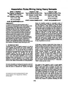
Figure 6. The generated decision tree

In this research, we implement two data types as a fuzzy set, namely alphanumeric and numeric. An example of alphanumeric data type is disease. We can define some meaningful fuzzy labels of disease, such as poor disease, moderate disease, and severe disease. Every fuzzy label is represented by a given fuzzy set. The age of patients is an example of numeric data type. Age may have some meaningful fuzzy labels such as young and old. Figure 6 shows an example result of FDT applied into three domains (attributes) data, namely Death, Age and Disease.

7. Conclusion The paper discussed and proposed a method to extend the concept of Decision Tree Induction using fuzzy value. Some generalized formulas to calculate information gain ware introduced. In the process of mining fuzzy association rules, some equations ware proposed to calculate support, confidence and correlation of a given association rules. Finally, an algorithm was briefly given to show the process how to generate FDT.

Acknowledgment This research was supported by research grant Hibah Kompetensi (25/SP2H/PP/DP2M/V/2009) and Penelitian Hibah Bersaing (110/SP2H/PP/DP2M/IV/2009) from Indonesian Higher Education Directorate.

References [1] J. Han, M. Kamber, Data Mining: Concepts and Techniques, The Morgan Kaufmann Series, 2001. [2] G. J. Klir, B. Yuan, Fuzzy Sets and Fuzzy Logic: Theory and Applications, New Jersey: Prentice Hall, 1995.

68


[3] R. Intan, “An Algorithm for Generating Single Dimensional Association Rules,”, Jurnal Informatika Vol. 7, No. 1, May 2006. [4] R. Intan, “A Proposal of Fuzzy Multidimensional Association Rules,”, Jurnal Informatika Vol. 7 No. 2, November 2006. [5] R Intan, “A Proposal of an Algorithm for Generating Fuzzy Association Rule Mining in Market Basket Analysis,”, Proceeding of CIRAS (IEEE). Singapore, 2005 [6] R. Intan, “Generating Multi Dimensional Association Rules Implying Fuzzy Valuse,”, The International Multi-Conference of Engineers and Computer Scientist, Hong Kong, 2006. [7] R. Intan, O. Y. Yuliana, “Fuzzy Decision Tree Approach for Mining Fuzzy Association Rules,”, 16th International Conference on Neural Information Processing, in be appeared, 2009. [8] O. P. Gunawan, Perancangan dan Pembuatan Aplikasi Data Mining dengan Konsep Fuzzy c-Covering untuk Membantu Analisis Market Basket pada Swalayan X, (in Indonesian) Final Project, 2004. [9] L. A. Zadeh, “Fuzzy Sets and systems,” International Journal of General Systems, Vol. 17, pp. 129-138, 1990. [10] R. Agrawal, T. Imielimski, A.N. Swami, “Mining Association Rules between Sets of Items in Large Database,”, Proccedings of ACM SIGMOD International Conference Management of Data, ACM Press, pp. 207-216, 1993. [11] R. Agrawal, R. Srikant, “Fast Algorithms for Mining Association Rules in Large Databases,”, Proccedings of 20th International Conference Very Large Databases, Morgan Kaufman, pp. 487-499, 1994. [12] H. V. Pesiwarissa, Perancangan dan Pembuatan Aplikasi Data Mining dalam Menganalisa Track Records Penyakit Pasien di DR.Haulussy Ambon Menggunakan Fuzzy Association Rule Mining, (in Indonesian) Final Project, 2005. [13] E.F. Codd, “A Relational Model of Data for Large Shared Data Bank,”, Communication of the ACM 13(6), pp. 377-387, 1970. [14] H. Benbrahim, B. Amine, “A Comparative Study of Pruned Decision Trees and Fuzzy Decision Trees,”, Proceedings of 19th International Conference of the North American, Atlanta, pp. 227-231, 2000. [15] Y. D. So, J. Sun, X. Z. Wang, “An Initial comparison of Generalization-Capability between Crisp and fuzzy Decision Trees,”, Proceedings of the First International Conference on Machine Learning and Cybernetics, pp. 1846-1851, 2002. [16] ALICE d'ISoft v.6.0 demonstration [Online]. Available at:http://www.alice-soft.com/demo/al6demo.htm [Accessed: 31 October 2007]. [17] Khoshgoftaar Taghi M., Y. Liu, N. Seliya “Genetic Programming-Based Decision Trees for Software Quality Classification,”, Proceedings of the 15th IEEE International Conference on Tools with Artificial Intelligence, California, pp. 374-383, 2003.

Authors Profile Rolly Intan obtained his B.Eng. degree in computer engineering from Sepuluh Nopember Institute of Technology, Surabaya, Indonesia in 1991. Now, he is a professor in the Department of Informatics Engineering at Petra Christian University, Surabaya, Indonesia. He received his M.A. in information science from International Christian University, Tokyo, Japan in 2000, and his Doctor of Engineering in Computer Science from Meiji University, Tokyo, Japan in 2003. His primary research interests are in data mining, intelligent information system, fuzzy set, rough set and fuzzy measure theory.

Oviliani Yenty Yuliana is an associate professor at the Department of Informatics Engineering, Faculty of Industrial Technology, Petra Christian University, Surabaya, Indonesia. She received her B.Eng. in Computer Engineering from Institut Teknologi Sepuluh Nopember, Surabaya, Indonesia. Her Master of Science in Computer Information System is obtained from Assumption University, Bangkok, Thailand. Her research interests are database systems and data mining.

Andreas Handojo obtained his B.Eng. degree in electronic engineering from Petra Christian University, Surabaya, Indonesia in 1999. He received his master, in Information Technology Management from Sepuluh November Institute of Technology, Surabaya, Indonesia, in 2007. Now, he is a lecturer in the Department of Informatics Engineering at Petra Christian University. His primary research interest are in data mining, business intelligent, strategic information system plan, and computer network.