Mining Image Datasets Using Perceptual Association Rules

Mining Image Datasets Using Perceptual Association Rules Jelena Teˇsi´c, Shawn Newsam and B. S. Manjunath Electrical and Computer Engineering Department University of California, Santa Barbara Santa Barbara, CA 93106-9560 {jelena, snewsam, manj}@ece.ucsb.edu Abstract This paper describes a framework for applying traditional data mining techniques to the non-traditional domain of image datasets for the purpose of knowledge discovery. In particular, perceptual association rules, a novel extension of traditional association rules, are used to distill the frequent perceptual events in large image datasets in order to discover interesting patterns. The focus is on spatial associations although the method is equally applicable to associations within or between other dimensions; i.e., spectral, or in the case of video, temporal. A primary contribution is the derivation of image equivalents for the traditional association rule components, namely the items, the itemsets, and the rules. The proposed approach is modular, consisting of three steps that can be individually adapted to a particular application. First, the image dataset is labeled in a perceptually meaningful way using a visual thesaurus. Second, the first- and second-order associations are tabulated in a scalable data structure termed a spatial event cube. Finally, the higher-order associations and rules are determined using an adaptation of the Apriori algorithm. The proposed approach is applied to an aerial video dataset to demonstrate the kinds of knowledge perceptual association rules can help discover.

1

Introduction

Multimedia data is being acquired at an increasing rate due to technological advances in sensors, computing power, and storage. The value of these sizable datasets extends beyond what can be realized by traditional “focused” computer vision solutions, such as face detection, object tracking, etc. Instead, new methods of analysis ∗ This research was supported in part by the following grants/awards: The Institute of Scientific Computing Research (ISCR) award under the auspices of the U.S. Department of Energy by the Lawrence Livermore National Laboratory under contract No.W-7405-ENG-48, Department of Transportation grant to the NCRST infrastructure at UCSB, ONR# N00014-01-10391, NSF Instrumentation #EIA-9986057, and NSF Infrastructure #EIA-0080134.

∗

based on data mining techniques are required to discover the implicit patterns, relationships and other knowledge that is not readily observable. Such knowledge is useful for a variety of applications, ranging from data summarization and visualization in scientific experimentation, to query refinement in multimedia data management systems. Data mining techniques have been used for some time to discover implicit knowledge in transaction databases. In particular, methods are available for determining the interesting associations among itemsets over large numbers of transactions, such as the products that are most frequently purchased together in market basket analysis. Achieving similar success with multimedia datasets remains a challenge, however, not only due to the size and complexity of image and video data, but also the lack of image equivalents for the association rule components, namely the items, the itemsets, and even the rules. It is not straightforward to define, let alone detect, the items and itemsets appropriate for discovering the implicit spatial knowledge contained in large collections of aerial images. The main contribution of this work is a framework for applying a specific set of traditional data mining techniques to the non-traditional domain of image datasets. In particular, perceptual association rules are proposed as a novel, multimedia extension to traditional association rules. 1.1 Motivation The objectives for applying association rule algorithms to traditional transaction databases are clear. A primary objective of market basket analysis is to determine optimal product placement on store shelves. However, the objectives for mining association rules in multimedia datasets are less obvious at this early stage in research on perceptual data mining when the limit of what is technically feasible are not known. Ideally, the rules would provide insight into the prominent trends in the dataset, such as interesting but non-obvious spatial or temporal causalities.

A spatial association rule derived from remote sensed imagery might help discover that two particular crops have a higher yield when planted near to each other. A strong motivation for the research presented in this paper is to investigate the kinds of knowledge perceptual association rules can help discover. This, in turn, will allow data mining practitioners to work with domain experts in identifying objectives that are both interesting and feasible. 1.2 Overview of the Proposed Approach An association rule [1] is an expression of the form A ⇒ B meaning the presence of itemset A implies the presence of itemset B. An association rule algorithm discovers the rules that have support and confidence larger than a specified threshold. The bottom-up approach proposed by this work transforms the raw image data into a form suitable for such analysis in three steps. First, image regions are labelled as perceptual synonyms using a visual thesaurus that is constructed by applying supervised and unsupervised machine-learning techniques to low-level image features. The region labels are analogous to items in transaction databases. Second, the first- and second-order associations among regions with respect to a particular spatial predicate are tabulated using spatial event cubes (SECs). The SEC entries are analogous to first- and second-order itemsets. Finally, higher-order associations and rules are determined using an adaptation of the Apriori association rule algorithm. These modular steps can be individually tailored, making the framework applicable to a variety of problems and domains The rest of the paper is organized as follows. Section 2 presents related work and Section 3 provides a general description of association rules and outlines a widely-used algorithm for discovering them. The proposed approach is described in Section 4 and experimental results for an aerial video dataset are presented in Section 5. Section 6 concludes with a discussion. 2 Related Work Several approaches to applying association rules to image datasets have been proposed. Ordonez and Omiecinksi [2] use segmentation results from the Blobworld system [3] to mine the co-occurrence of image regions that have been labeled as similar using an empirically determined distance measure and threshold. The segmented regions are viewed as items and the images are viewed as transactions so that the resulting rules are of the form, “The presence of regions A and B imply the presence of region C with support X and confidence Y”. It is not clear, however, that the results from applying the technique to a dataset of synthetic images composed

of basic colored shapes would generalize to real images for which segmentation and notions of region similarity present a significant challenge. Ding et al. [4] extract association rules from remote sensed imagery by considering set ranges of the spectral bands to be items and the pixels to be transactions. They also consider auxiliary information at each pixel location, such as crop yield, to derive association rules of the form “Band 1 in the range [a, b] and band 2 in the range [c, d] results in crop yield Z with support X and confidence Y.” However, analysis at the pixel scale is susceptible to noise, unlikely to scale with dataset size, and limited in its ability to discover anything other than unrealistically localized associations-i.e., in reality, what occurs at one pixel location is unlikely to be independent of nearby locations. 3 Association Rules This section provides a general description of association rules and outlines a widely used algorithm to discover them. Association rule approach was first introduced in [1] as a way of discovering interesting patterns in transactional databases. An association rule tells us about the association between two or more items. Let U = {u1 , ...uN } be set of items. A set A is a K −itemset, if A ⊆ U and |A| = K. An association rule is an expression A ⇒ B, where A and B are itemsets that satisfy A ∩ B = Ø. Lets D as a superset, i.e. D = {T |T ⊆ U }. Elements of database D are called transactions. Transaction T ⊆ D supports an itemset A if A ⊆ T . Support of itemset A over all database transactions T is defined as: |{T ∈ D|A ⊆ T }| |D| Apriori algorithm discovers combination of items that occur together with greater frequency than might be expected if the values or items were independent. The algorithm selects the most “interesting” rules based on their support and confidence. Rule A ⇒ B expresses that whenever a transaction T contains A, it probably contains B also. Support measures statistical significance of a rule: (3.1)

supp(A) =

|{T ∈ D|A ⊆ T ∧ B ⊆ T }| |D| Confidence is a measure of a strength of a rule:

(3.2)

supp(A ⇒ B) =

|{T ∈ D|A ⊆ T ∧ B ⊆ T }| |{T ∈ D|A ⊆ T }| The probability of rule confidence is defined as conditional probability p(B ⊆ T |A ⊆ T ). Association rules can be between more than 2 items, i.e. A, B ⇒ C where A, B, C ⊆ U . Association rule is strong if its confidence is larger than user’s specified minimum support. (3.3)

conf (A ⇒ B) =

Several improvements have been proposed for mining association rules [5]. They deal with complexity of rule mining and separating interesting rules from the generated rule set in a more efficient way. The user has to specify minimum support of frequent itemsets. Every subset of a frequent itemset is also frequent. An itemset can be frequent only if it is frequent in at least one of these partitions and algorithm takes advantage of that property. The Apriori algorithm identifies frequent itemsets as following: Algorithm 1 Apriori Algorithm 1. Find frequent item sets; F1 = {ui | kui k > minimum support} for (K = 2; FK−1 6= Ø; K + +) do CK = {ck |c(a) ∧ c(b) ∈ FK−1 }, where: ck = (ui1 , ..., uik−2 , uik−1 , uik ) c(a) = (ui1 , ..., uik−2 , uik−1 ) c(b) = (ui1 , ..., uik−2 , uik ) kck k = 0; for (∀T, T ⊆ D) and (∀ck , ck ∈ CK ) do if (ck ∈ T ) then kck k = kck k + 1; end if end for FK = {ck |kck k > minimum support } end S for F = K FK 2. Use the frequent itemsets to generate strong association rules. 4 Perceptual Association Rules This section describes the three steps of the proposed approach: 1) perceptual labeling of the image regions using a visual thesaurus; 2) tabulation of first- and second-order associations using SECs; and 3) mining of higher-order associations and rules.

perceptual synonyms of the visual thesaurus. The image dataset is then labeled by assigning each region the codeword of its entry in the thesaurus. More details on the visual thesaurus and its construction can be found in [6]. 4.2 Spatial Event Cubes The visual thesaurus is used to label the image regions based solely on their distribution in the feature space. Knowledge of the spatial arrangement of the regions is incorporated through SECs, a scalable data structure that tabulates the region pairs that satisfy a given binary spatial predicate, see [7]. Define the raster space R for an image partitioned into M × N tiles as R = {(x, y)| x ∈ [1, M ], y ∈ [1, N ]}. Let the set of T of thesaurus entries ui be: T = {ui |ui is a thesaurus entry/codeword}. Let τ be a function that maps image coordinates to thesaurus entries, τ (P ) = u, where P ∈ R and u ∈ T ; and let ρ be the given binary spatial predicate, P ρQ ∈ {0, 1}, where P, Q ∈ R. Then, an SEC face is the co-occurrence matrix Cρ (u, v) of all pairs of points that have codeword labels u and v, and satisfy the binary predicate ρ: Cρ (u, v) = k(P, Q)| (P ρQ) ∧ (τ (P ) = u) ∧ (τ (Q) = v)k These co-occurrences are computed over all the images in the dataset. Note that it is the relation ρ that determines the particular spatial arrangement tabulated by the SEC. The choice of ρ is application dependent and can include spatial relationships such as adjacency, orientation, and distance, or combinations thereof.

4.3 Perceptual Association An attribute value set T contains N thesaurus entries ui . Spatial Event Cube face entries Cρ (u, v) mark frequency of codeword tuples that satisfy binary relation ρ ρ. Define FK as a set of frequent itemsets of size K. Also define Sρ as a minimum support value for 4.1 Perceptual Labeling using a Visual The- frequency of Cρ (ui1 , ..., uiK ). Our goal is to find sets of tuples that show some among tile spatial saurus S dependency ρ ρ A visual thesaurus is used to label the image regions configurations. F = K FK . Since the Spatial Event in a perceptually meaningful way. The visual thesaurus Cube captures spatial relationship only between two is constructed in two stages using the low-level region tiles, we need to implement some clever processing to features and a manually labeled training set. First, the build higher order candidates. Spatial relationship for dimensionality of the feature space is reduced by feeding K − −itemsets depends on the characteristics of binary the training set into a self-organizing map (SOM), function ρ. Perceptual Association Rule Algorithm supports a clustering technique that is known to preserve the topology of the input space. The resulting clusters atomic pattern set approach to candidate itemset generare assigned class labels using a majority-vote rule and ation in multimedia datasets [8]. We test occurrences of the SOM is used to classify the entire dataset. The interesting patterns in a dataset, thus avoiding the forsecond stage fine-tunes these classes using an improved mulation of transactions. A set of atomic patterns for (1) Learning Vector Quantization (LVQ) algorithm. The our representative dataset D is F1 = {ui | kui k > Sρ }. resulting sub-classes group the region features into the For F2 we build the conjunction of two atomic patterns

(ui , uj ) and look for the corresponding SEC entries. If (2) Cρ (ui , uj ) > Sρ , then (ui , uj ) ∈ F2 . Spatial Event Cubes are built on a binary relationship ρ. For higher order candidate sets we are imposing a clever processing rule i.e. ordering. Then, we go back to representative dataset D and record the occurrences of new candidates, as explained in the previous paragraph. Only the ones with support larger that the user specified minimum (K) Sρ qualify for the frequent itemset of size k. Note that the clever processing rule can differ for a different itemset size. If we have more elements in an itemset, there are more ways to spatially organize those elements. Association rules can be between 3 items is in the form ui , uj ⇒ uk where ui , uj , uk ⊆ D. If Cρ (ui , uj , uk )/Cρ (ui , uj ) is larger than minimum confidence required, the rule ui , uj ⇒ uk is a valid rule. For the right neighbor example, this rule could be formulated as “If codeword uj is right neighbor of codeword ui , that might imply that uk is on the right side of uj ”. Extended association rule algorithm for spatial relationship ρ is: Algorithm 2 Perceptual Association Rule 1. Find frequent item sets (1) F1ρ = {ui | kui k > Sρ }; (2) ρ F2 = {(ui , uj )|Cρ (ui , uj ) > Sρ }; for (K = 3; FK−1 6= Ø; K + +) do Candidate K-item frequent itemset CK is formed of K ρ item set; joint elements from any frequent FK−1 (a) (b) CK = {ck |c , c ∈ FK−1 }, where: ck = (ui1 , ..., uik−2 , uik−1 , uik ) c(a) = (ui1 , ..., uik−2 , uik−1 ) c(b) = (ui1 , ..., uik−2 , uik ) for (∀k, ck ∈ CK ) and (∀i, σi ∈ RK ) do kck k = k{σi |σi satisfies spatial relationship}k AND (τ (P1 ) = u1 ) ∧ ... ∧ (τ (PK ) = uK ), where σi = (P1 , ..., PK ), (P1 , ..., PK ) ∈ RK end for (K) FK = {ck |kck k > Sρ } end for S ρ F ρ = K FK 2. Use the frequent itemsets to generate association rules;

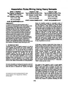
Figure 1: Training set samples. From top to bottom row: pasture, forest, agriculture, road, and urban agery. It is particularly attractive for areas plagued by cloud cover, such as the Amazon, since the aircraft are flown at low altitudes. The sample dataset was captured using a high-end commercial video camera and is geo-referenced. The aerial videos are temporally subsampled to create a sequence of just-overlapping frames, which are treated as a collection of images. One hour of video results in approximately 450 frames of size 720 by 480 pixels. Figure 3(a) shows a sample frame. The results presented here are for one hour of the 40-hour dataset. The proposed method can alternately be applied to image mosaics created from the video although care must be taken that the mosaicking process does not introduce unwanted artifacts.

5.1 Homogeneous Texture Descriptor The raw image data is perceptually characterized using a low-level descriptor based on homogeneous texture. The Vision Research Lab at UCSB has extensive experience with using texture to analyze remote sensed imagery. In particular, an MPEG-7 [9] compliant descriptor based on the outputs of orientation– and scale–selective Gabor filters [6] has shown to effec5 Experimental Results tively characterize a variety of land cover types, such The proposed technique is applied to a collection of as agriculture, forest, and urban development. Since aerial videos of Amazonia made available by the Insti- the texture descriptor captures the spatial distribution tute for Computational Earth System Science (ICESS) of relative pixel values, it is less sensitive to changes in at UCSB. Aerial videography is an affordable alterna- lighting conditions than spectral descriptors. This turns tive to expensive high-resolution aerial and satellite im- out to be a significant advantage for analyzing the aerial

(a) Rotation sensitive retrieval

(b) Rotation invariant retrieval

Figure 2: Similarity retrieval based on a distance function Class 0 1 2 3 4

Description Pasture Forest Agricultural Road Urban

Training Set Size 285 238 116 185 116

Table 1: Training set for 5 class manual labeling. Total Number of Training Tiles is 940

mary land cover types are identified as pasture, forest, water, agricultural, and urban. Water is not considered separately since it does not occur often and is similar to clear pasture with respect to the texture. Roads occur frequently and are distinct so the final basic land cover types are pasture, forest, agricultural, road, and urban. Table 5.1 lists the size of the five classes in the training set. Note that the training set measures less than three percent of the entire dataset. Figure 1 shows sample tiles from the training set. The LVQ stage of the training algorithm results in a visual thesaurus with 73 codewords. These codewords can be considered as fine tuned subclasses of the manually chosen training classes. Figures 3(b) and 3(c) show the results of using the visual thesaurus to label the frame in Figure 3(a). Figure 3(b) shows the class assignments, which are mostly correct. Figure 3(c) shows the codeword labels, which are subclasses of the training set labels. For example, codeword labels 0 through 19 correspond to subsets of the pasture class, and labels 49 through 63 correspond to subsets of the road class. This demonstrates a key feature of the visual thesaurus: the final codeword labeling represents a finer and, therefore, more consistent partitioning of the high dimension feature space than the manually chosen training set.

videos of Amazonia, which contain a mixture of sunny and cloud-shaded regions. The texture descriptors are extracted in an automated fashion by dividing the video frames into nonoverlapping 64 by 64 pixel tiles and applying Gabor filters tuned to combinations of six orientations and five scales. The first– and second–order moments of the filter outputs form the texture feature vector. Thus, one hour of video results in approximately 35,000 tiles each characterized by a 60-dimension vector. The visual similarity between tiles is computed by defining a distance function on the high-dimensional feature space. Euclidean distance results in an orientation– and scale– selective similarity measure. Invariant similarity is measured using a distance function that exploits the structure of the feature vectors [10]. Figure 2 shows examples of both orientation-selective and orientation-invariant similarity retrieval.The visual thesaurus is constructed using the 5.3 Spatial Event Cubes invariant similarity measure since the image regions oc- An SEC is computed from the codeword labeled frames cur at arbitrary orientations in the aerial videos. using 8-neighbor adjacency as the spatial predicate. The diagonal entries of the SEC indicate the number of times 5.2 Visual Thesaurus a codeword appears next to itself. The visual thesaurus is used to label the video frame Thus, the largest diagonal values correspond to the tiles in a perceptually meaningful way by clustering the homogeneous regions of the dataset. Table 2 lists the high-dimensional texture feature vectors using super- diagonal entries with the largest values. These entries vised and unsupervised learning techniques. The train- correspond to pasture and forest codewords. ing set required by the supervised learning stage is manA second SEC is computed this time using a direcually chosen with the help of domain experts. The pri-

(a) Extracted frame No. 238

(b) Labeled frame - 5 classes

(d) 21

(e) 0

(f) 35

(g) 12

(h) 17

(i) 33

(j) 24

(k) 41

i 21 0 35 12 17 33 24 41 4 38

(c) Labeled frame - 73 codewords

kui k 3621 2555 2330 2903 2081 1183 884 943 1289 728

Cρ (ui , ui ) 2366 2273 1608 1566 1054 796 508 508 492 450

Cρ (ui , ui )/kui k 0.653411 0.889628 0.690129 0.539442 0.506487 0.672866 0.575226 0.538706 0.382079 0.618819

Table 2: Corresponding Frequencies of largest diagonal SEC entries for 8-connectivity neighborhood (l) 4

(m) 38

(n) 9

(o) 13

Figure 3: Thesaurus codewords for the most frequent elements of F2ρ tional spatial adjacency predicate ρ: (x1 , y1 )ρ(x2 , y2 ) ⇔ (x1 = x2 ) ∧ (y1 + 1 = y2 ),

i 12 17 35 17 12 35 38 21

j 0 12 33 4 9 24 24 13

Cρ (ui , uj ) 2461 1764 1095 939 876 781 601 571

conf(ui ⇒ uj ) 0.423872 0.423835 0.234979 0.225613 0.150878 0.167597 0.412775 0.078846

conf(uj ⇒ ui ) 0.481605 0.303824 0.462806 0.364236 0.344611 0.441742 0.339932 0.402113

where xi and yi are the horizontal and vertical coordinates of tile i. This predicate allows spatial analysis Table 3: Confidence of generated rules from F2ρ set along the direction of flight of the aerial video. Table 4 lists the diagonal entries with the largest values. These entries correspond to pasture and forest codewords. range 0 through 19 correspond to pasture subclasses and codewords in the range 20 through 39 correspond 5.4 Itemsets and Rules to forest subclasses. The support 3.2 and confidence 3.3 of constructed rule While it is no surprise that forest and pasture ui ⇒ uj for 8-connectivity neighborhood can be derived are the most frequently occurring land types, table from the SEC entries: 3 indicates that specifically forest codeword 21 and C (ui ,uj ) pasture codeword 0 occur most frequently. Pasture supp(ui ⇒ uj ) = ρ |D| codeword 13 is more likely to occur next to forest Cρ (ui ,uj ) conf (ui ⇒ uj ) = 2∗|ui | codeword 21 than vice versa. For the second SEC, constructed associated rules A factor of two is needed in the denominator in this case from F2ρ are listed in tables 4 and 6, respectively. note since ρ is symmetric. Constructed associated rules from F2ρ are listed that the confidence of constructed rule ui ⇒ uj for in tables 2 and 3, respectively. The corresponding “righthand neighborhood rule” is: confidence values are also indicated. Figure 3 shows the C (ui ,uj ) supp(ui ⇒ uj ) = ρ |D| corresponding codewords to the most frequent elements C (u ,u ) conf (ui ⇒ uj ) = ρ |uii | j of the second order item set F2ρ . Codewords in the

i 21 0 35 12 17 33 24 41 4 38

kui k 3621 2555 2330 2903 2081 1183 884 943 1289 728

Cρ (ui , ui ) 1159 1093 677 1760 425 329 191 209 225 167

Cρ (ui , ui )/kui k 0.320077 0.427789 0.290558 0.261798 0.204229 0.278107 0.216063 0.221633 0.174554 0.229396

Table 4: Corresponding Frequencies of largest diagonal SEC entries for the “righthand neighbor” spatial rule

(12, 0, 0) (9, 12, 12) (21, 35, 35) (21, 17, 0)

conf ((12, 0) ⇒ 0) = 0.23077 conf ((9, 12) ⇒ 12) = 0.23737 conf ((21, 35) ⇒ 35) = 0.27708 conf ((12, 17) ⇒ 0) = 0.095

Table 5: Confidence of generated rules from F3ρ set, for the “righthand neighbor” rule Since these results are almost identical to the ones for 8-neighborhood adjacency, it can be concluded that the dataset is isotropic with respect to adjacency. Mining rule for third order itemset is formulated as “If codeword uj is right neighbor of codeword ui , that implies that uk is on the right side of uj with confidence conf((ui , uj ) ⇒ uk )”. We constrained the candidates in C3ρ to form a “righthand neighbor” chain. Constructed associated rules from F3ρ are listed in table 5. 6 Conclusion In this paper, we introduce an association rule mining framework that supports spatial event discovery in large image datasets. Feature vectors are extracted from image tiles and summarized into visual thesaurus. Visual thesaurus allows us to record spatial relationships among labelled features using Spatial Event Cube (SEC) approach. SEC support perceptual association rule mining approach and provide efficient pruning for generating higher order candidate itemsets. We demonstrate the use and possible applications of proposed framework on a large collection of aerial videos of Amazonia and large collection aerial photos of Santa Barbara region. Future research include implementation of mining more complex spatial rules and a cost function that will prove the efficiency of the proposed method. We are also planning to use Spatial Event Cubes as an index structure for multimedia database access.

i 0 12 21 35 17 12 35 33 12 9 17

j 12 0 35 21 12 17 33 35 9 12 4

Cρ (ui , uj ) 521 507 480 442 346 335 227 208 202 198 185

conf(ui ⇒ uj ) 0.203914 0.174647 0.132560 0.189700 0.166266 0.115398 0.097425 0.175824 0.069583 0.155783 0.088900

conf(uj ⇒ ui ) 0.179470 0.198434 0.206009 0.122066 0.119187 0.160980 0.191885 0.089270 0.158930 0.068205 0.143522

Table 6: Confidence of generated rules from F2ρ set, for the “righthand neighbor” rule 7 Acknowledgments The authors would like to thank Chandrika Kamath and Imola K. Fodor for many fruitful discussions. References [1] R. Agrawal and R. Srikant, “Fast algorithms for mining association rules,” in Proc. 20th Int’l Conf. Very Large Data Bases (VLDB), 1994. [2] C. Ordonez and E. Omiecinski, “Discovering association rules based on image content,” in Proc. IEEE Advances in Digital Libraries Conference (ADL), 1999. [3] C. Carson, S. Belongie, H. Greenspan, and J. Malik, “Region-based image querying,” in Proc. CVPR ’97 CBAIVL Workshop, 1997. [4] Qin Ding, Qiang Ding, and William Perrizo, “Association rule mining on remotely sensed images using p-trees,” in Proc. PAKDD, 2002. [5] J. Han and Y. Fu, “Discovery of multiple-level association rules from large databases,” in Proc. 21st Int’l Conf. Very Large Data Bases (VLDB), 1995. [6] W. Ma and B. S. Manjunath, “A texture thesaurus for browsing large aerial photographs,” Journal of the American Society of Information Science, 1998. [7] J. Teˇsi´c, S. Newsam, and B.S. Manjunath, “Scalable spatial event representation,” in Proc. IEEE Int. Conf. on Multimedia and Expo (ICME), 2002. [8] D. J. Hand, H. Mannila, and P. Smyth, Principles of DataMining, MIT Press, Cambridge, MA, 2000. [9] B.S.Manjunath, P. Salembier, and T. Sikora, Eds., Introduction to MPEG7: Multimedia Content Description Interface, John Wiley & Sons, 2002. [10] S. Newsam and B.S.Manjunath, “Normalized texture motifs and their application to statistical object modeling,” in Submitted to ICCV, 2003.