Mining Iterative Generators and Representative Rules for Software

1

Mining Iterative Generators and Representative Rules for Software Specification Discovery David Lo, Member, IEEE, Jinyan Li, Limsoon Wong, and Siau-Cheng Khoo Abstract—Billions of dollars are spent annually on software related cost. It is estimated that up to 45% of software cost is due to the difficulty in understanding existing systems when performing maintenance tasks (i.e., adding features, removing bugs, etc.). One of the root causes is that software products often come with poor, incomplete or even without any documented specifications. In an effort to improve program understanding, Lo et al. have proposed iterative pattern mining which outputs patterns that are repeated frequently within a program trace, or across multiple traces, or both. Frequent iterative patterns reflect frequent program behaviors that likely correspond to software specifications.To reduce the number of patterns and improve the efficiency of the algorithm, Lo et al. have also introduced mining closed iterative patterns, i.e., maximal patterns without any super-pattern having the same support. In this paper, to technically deepen research on iterative pattern mining, we introduce mining iterative generators, i.e., minimal patterns without any sub-pattern having the same support. Iterative generators can be paired with closed patterns to produce a set of rules expressing forward, backward and in-between temporal constraints among events in one general representation. We refer to these rules as representative rules. A comprehensive performance study shows the efficiency of our approach. A case study on traces of an industrial system shows how iterative generators and closed iterative patterns can be merged to form useful rules shedding light on software design. Index Terms—Frequent Pattern Mining, Sequence Database, Iterative Patterns, Generators, Representative Rules, Software Engineering (Reverse Engineering and Program Comprehension).

F

1

I NTRODUCTION

AND

M OTIVATION

It is best if software is developed with clear, precise and documented specifications. However, due to hard deadlines and ‘short-time-to-market’ requirement, software products often come with poor, incomplete and even without any documented specifications. This situation is further aggravated by a phenomenon termed software evolution [1]. As software evolves, the documented specifications often remain unchanged [2]. This might render the documented specification of little use after cycles of program evolution. These factors have contributed to high software maintenance cost. It has been reported that up to 90% of software cost is due to maintenance [3] and up to 50% of the maintenance cost is due to the effort put in comprehending or understanding software code base [4]. Hence, approximately up to 45% of software cost is due to the difficulty in comprehending an existing code base. This is especially true for software projects developed by many developers over a long period of time. These needs motivate work on automated tools to extract or mine specifications from programs. An interesting form of specifications to be mined is patterns of software temporal behaviors. These patterns are intuitive and commonly found • D. Lo is with the School of Information Systems, Singapore Management University, 80 Stamford Road, Singapore 178902. Email: [email protected]. • J. Li is with the School of Computer Engineering, Nanyang Technological University, Nanyang Avenue, Singapore 639798. Email: [email protected]. • L. Wong and S-C. Khoo are with the School of Computing, National University of Singapore, Building COM1, Law Link, Singapore 117590. Email: {wongls,khoosc}@comp.nus.edu.sg.

in software documentations. Some examples are as follows: 1) Resource Locking Protocol : hlock, unlocki 2) Telecommunication Protocol (c.f., [5]): hoff hook, dial tone on, dial tone off, seizure int, ring tone, answer, connection oni 3) Java Authentication and Authorization Service (JAAS) Authorization Enforcer Strategy Pattern (c.f., [6]): hSubject.getPrincipal, PrivilegedAction.create, Subject.doAsPrivileged, JAAS Module.invoke, Policy.getPermission, Subject.getPublicCredential, PrivilegedAction.runi 4) Java Transaction Architecture (JTA) Protocol (c.f., [7]): hTxManager.begin, TxManager.commiti, hTxManager.begin, TxManager.rollback i Each of these patterns reflects an interesting program behavior. It can be mined by analyzing a set of program traces – each being a series of method invocations. These program traces can in turn be generated through running a test suite. From data mining viewpoint, each trace can be considered a sequence. A pattern (e.g., lock-unlock) can appear a repeated number of times within a sequence. Each event can be separated by an arbitrary number of unrelated events (e.g., lock → resource use → . . . → unlock). Since a program behavior can be manifested in numerous ways, analyzing a single trace will not be sufficient. To mine software temporal patterns having the above characteristics from traces, Lo et al. proposed iterative pattern mining [8] which extends sequential pattern mining and episode mining to address software specification mining. Sequential pattern mining first addressed by Agrawal and Srikant in [9] discovers temporal patterns that are supported

2

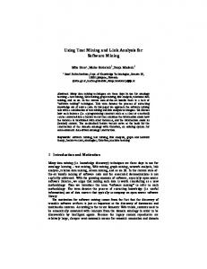
by a significant number of sequences. A pattern is supported by a sequence if it is a sub-sequence of it. It has application in many areas, from analysis of market data to gene sequences. On the other hand, Mannila et al. propose episode mining to discover frequent episodes within a sequence of events [10]. An episode is defined as a series of events occurring relatively close to one another (e.g., they occur at the same window). An episode is supported by a window if it is a sub-sequence of the series of events appearing in the window. Episode mining focuses on mining from a single sequence of events. Frequent iterative pattern is a series of events supported by a significant number of instances repeated within and across sequences. Similar to sequential pattern mining, we consider a database of sequences rather than a single sequence. However, we also mine patterns occurring repeatedly within a sequence. This is similar in spirit to episode mining, but we remove the restriction that related events must happen in the same window. Due to looping, a trace can contain repeated occurrences of interesting patterns. In fact, a series of events in an alarm management system used by Manilla et al. is similar to a series of system calls in a software system. However, there are 2 notable differences. First, program properties are often inferred from a set of traces instead of a single trace. These are either produced by executing a test suite or generated statically from the source code. Secondly, important patterns for verification, such as lock acquire and release or stream open and close, often have their events occur at some arbitrary distance away from each other in a program trace. Hence, there is a need to ‘break’ the ‘window barrier’ in order to capture these patterns of interest. Interestingly, these two notable differences between analysis of events from an alarm management system and program traces are observed by sequential pattern miner first introduced in [9]. To support iterative pattern mining, we need a clear definition and semantics of iterative pattern different from that of episode and sequential pattern. Our definition of iterative pattern is inspired by common languages for specifying software behavioral requirements, namely Message Sequence Chart (MSC) [5] and Live Sequence Chart (LSC) [11]. MSC and LSC are variants of sequence diagram specifying how a system should behave. An example of such a chart is a simplified telephone switching protocol shown in Figure 1 – c.f., [5]. Abstracting caller and callee information, it can be represented as a pattern: hoff hook, dial tone on, dial tone off, seizure int, ring tone, answer, connection oni. Switching Sys Calling Called Party Party off_hook dial_tone_on dial_tone_off seizure ack ring_tone answer connection

Fig. 1. Simplified Telecommunication Protocol.

Pattern mining in general is an NP-hard problem. For it to be practical, efficient search space pruning strategies need to be employed. In [8], Lo et al. address the issue by mining a closed set of iterative patterns. In this work, we investigate mining of iterative generators from program execution traces. Generators are the minimal members of an equivalence class, while closed patterns are the maximal members. An equivalence class in turn is a set of frequent patterns with the same support and corresponding pattern instances. The concept of generator has been applied to frequent itemsets [12], [13], [14] and sequential patterns [15]. We propose an approach to mine generators of iterative patterns. Unless otherwise stated, in this paper, generators refer to iterative generators. We find that the algorithms mining closed iterative patterns and sequential generators can not be trivially extended to mine iterative generators as major properties used for mining closed iterative patterns and sequential generators no longer apply for iterative generators. The set of closed patterns and generators are potentially of much smaller size than the full-set of frequent patterns. As generators are minimal members of equivalence classes, according to the Minimum Description Length (MDL) principle, generators are the preferred descriptors for the “encoding” of the classes. Also, as argued by Li et al, generators are better candidates than closed patterns for applications involving model selection and classification [13]. Furthermore, closed iterative patterns and generators can be merged to form a compact knowledge representation capturing an expressive form of temporal constraints. These constraints are in the form of rules with minimal pre-conditions and maximal post-conditions referred to as representative rules. Temporal constraints add more information to patterns and are useful in software domain as they correspond to temporal properties used to find bugs and ensure correctness of systems via formal verification tools [16]. Past studies on mining rules have focused on finding forward temporal constraints (i.e., if a series of events occurs, eventually another series of events occurs) [17], [18] or backward temporal constraints (i.e., if a series of events occurs, previously, another series of events has occurred before) [19]. A representative rule on the other hand captures a more general form of temporal constraints. It first describes a sequence of pre-condition events which, if satisfied, implies the occurrence of other events which can happen before, in-between or after the sequence of pre-condition events. Aside from being more compact, representative rules capture in-between temporal constraints which are not expressible by combining forward or backward temporal constraints. For example, consider the rule hX, {A}, Y, {B}, Zi, where the ones marked with brackets correspond to the pre-condition events. This rule states that when the events A and B occur, X must happen before A, Y must happen in between A and B and Z must happen after B. The rule captures not only forward temporal constraints but also backward and inbetween temporal constraints. As a visual representation, one can imagine the horizontal arrows in Figure 1 be drawn in two different colors, one representing the pre-condition and

3

the other the post-condition. The utility of the general format of representative rules is readily evident in daily life. Consider an Automated Teller Machine (ATM), one important property is: “a user must be authenticated after an ATM card is inserted and before money is dispensed”, i.e., h{ins card}, authenticate, {dis money}i. Also, consider a university, an important property is: “a student must pass all the examinations after he/she is matriculated and before he/she graduates”, i.e., h{matriculate}, pass exams, {graduate}i. Consider an example temporal constraint used to verify correctness of Windows device drivers: a driver that has called KeAcquireSpinLock , KeInsertDeviceQueue and eventually KeReleaseSpinLock , must have called IoMarkIrpPending after the call to KeInsertDeviceQueue, but before the call to KeReleaseSpinLock , i.e., h{KeAcquireSpinLock }, {KeInsertDeviceQueue}, IoMarkIrpPending, {KeReleaseSpinLock }i – c.f. [20]. These types of temporal constraints can be mined by mining representative rules but not by the previous studies on rule mining which only mine either forward or backward temporal constraints separately. To mine iterative generators, we introduce the concept of approximate iterative pattern. An approximate pattern weakens the constraint that a regular pattern imposes on its instances. We introduce approximate patterns since we can obtain the set of frequent patterns with correct support from them and they have a good property which can be utilized to avoid redundant efforts when traversing the search space of frequent patterns. The support of an approximate pattern is an upper bound of the actual pattern support. We first construct a compact lattice representing frequent approximate patterns by building it depth-first. Redundant search space traversal efforts are avoided by detection of equivalent sub-lattices. If a sub-lattice is equivalent to an existing sub-lattice there is no need to build it again. Next, we traverse the compact lattice breadth-first while performing: (1) Computation of real pattern support, (2) Identification of generators, and (3) Pruning of sub-search-spaces containing only non-generators. After the steps above are performed, a set of generators would be mined. The generators are then merged with closed patterns to produce a set of representative rules capturing forward, backward and in-between temporal constraints. A performance and a comparative study are conducted on synthetic and real benchmark datasets to evaluate the performance of the proposed mining algorithm. The proposed algorithm can run efficiently at low support thresholds, large number of sequences and reasonably long sequences on 10 synthetic and 2 real benchmark datasets. The experiments also show that iterative generators can be mined with similar efficiency as closed patterns. Since, both generators and closed patterns are needed to form representative rules capturing forward, backward and in-between temporal constraints we need to ensure that both algorithms run at least with similar efficiency. It is not our purpose to beat the efficiency of closed iterative pattern mining algorithm. As a case study, we extend the study on JBoss Application Server (JBoss AS) in [8]. The mined generators combined

with mined closed patterns form interesting rules that shed further light on the behavior of the software system expressing forward, backward and in-between temporal constraints that the system obeys. The contributions of this work are as follows: 1) We propose iterative generators and representative rules as new data mining concepts for software specification discovery. 2) We present novel properties of iterative generators for: (i) generator identification, (ii) search-space compaction, and (iii) non-generator pruning. 3) We propose a new algorithm to mine iterative generators and generate representative rules. Different from past algorithms on mining from sequences of events, we introduce: (i) A merge between depth-first and breadthfirst traversal of search space, (ii) A new lattice data structure, and (iii) New techniques to detect equivalences of projected databases, compute real support and utilize the properties of iterative generators for their efficient mining. The outline of the paper is as follows: Section 2 presents related work. Section 3 provides preliminary information on notations, semantics of iterative pattern and definitions of closed pattern and generator. An analysis on the need for a new algorithm to mine iterative generators is also described in the section. Section 4 presents approximate iterative pattern and the approximate pattern lattice data structure. The section also discusses some properties of approximate patterns for effective search space compaction. Furthermore, some properties for efficient pruning of iterative generators are also discussed in this section. Section 5 describes our iterative generator mining algorithm and representative rule generation process. Section 6 presents the results of our performance study. Section 7 presents the case study on JBoss AS. We discuss interesting issues and future work in Section 8.

2

R ELATED W ORK

Iterative pattern mining is an extension of sequential pattern mining, which was first proposed by Agrawal and Srikant [9]. To remove redundant patterns, closed sequential pattern mining was proposed by Yan et al. [21]. The approach was later improved by Wang and Han [22]. Different from sequential pattern, iterative pattern captures multiple occurrences of pattern not only across multiple sequences but also those repeated within each sequence. In this aspect, iterative pattern mining resembles episode mining initiated by Mannila et al. [10] which was later extended by Casas-Garriga to replace a fixedwindow size with a gap constraint between one event to the next in an episode [23]. Both versions of episode mining mine events occurring close to one another, expressed by “window size” and gap constraint respectively. This is different with iterative pattern mining, which does not have the notion of an “episode”. This difference is significant, since important program behavioral patterns, for example: lock acquire and release, or file open and close, often have their events occur at some arbitrary distance away from one another in a trace. In addition, both versions of episode mining handle only one

4

sequence, while iterative pattern mining operates over a set of sequences. There are also other studies on mining patterns that repeat in sequences. In mining DNA sequences, Zhang et al. introduced the idea of “gap requirement” in mining periodic patterns from sequences [24]. Similar to ours, they detect repeated occurrences of patterns within a sequence and across multiple sequences. However, the gap requirement used in their work does not always hold for other purposes. Consider analyzing software traces, the useful patterns of lock-acquire followedby lock-release can be separated by any number of events, and will violate the gap requirement. Recently, Ding et al. mine for closed repetitive sub-sequences [25]. Different from their work, we consider the minimal patterns in equivalence classes (i.e., generators) rather than the maximal patterns in equivalence classes (i.e., closed patterns). Also, the semantics of Zhang et al.’s periodic pattern and Ding et al.’s repetitive subsequence differ from iterative pattern that follows MSC/LSC. In [8], Lo et al. mine all frequent and closed iterative patterns. In this work, we mine for iterative generators.Closed patterns are the maximal patterns in the equivalence classes of patterns having the same support while generators are the minimal patterns. There are also several studies on mining generators. Pasquier et al. mine generators of frequent itemsets [12]. In [13], Li et al. improve the algorithm in [12]. In [14], Li et al. extend their work by concurrently obtaining both closed itemsets and generators, and computing delta discriminative non-redundant equivalent classes. Lo et al. mine a set of sequential generators [15]. A concurrent study on mining sequential generators is also made by Gao et al. in [26]. Different from the above studies, we mine iterative generators which poses further challenges since repeated occurrences of patterns within a sequence need to be considered. Furthermore, the definition of iterative pattern instances follows the semantics of MSC/LSC that involves negation. There are past studies on mining rules from sequences of events [17], [27], [28], [18], [19]. There are a number of differences between our work and each of them. Most importantly, the proposed representative rules are able to specify forward, backward and in-between temporal constraints in one representation and they can be mined efficiently.

3

P RELIMINARIES

In this section, we define some notations, outline the semantics of iterative patterns and describe the definitions of closed iterative patterns and iterative generators. An analysis on the need for a new algorithm to mine iterative generators is also presented. 3.1 Basic Definitions Let I be a set of distinct events. In this work, the events of interest are method calls that are invoked when a program is executed. Thus, a call to a unique method would correspond to a unique event. Let a sequence S be a series of events. We denote S as he1 , e2 , . . . , eend i where each ei is an event from I. The sequence database under consideration is denoted

by DB. The ith sequence in the database DB is denoted as DB[i]. Also the jth position of the sequence DB[i] is denoted as DB[i][j]. A pattern P1 = he1 , e2 , . . . , en i is considered a subsequence of another pattern P2 = hf1 , f2 , . . . , fm i if there exist integers 1 ≤ i1 < i2 < i3 < i4 . . . < in ≤ m where e1 = fi1 , e2 = fi2 , · · · , en = fin . Notation-wise, we write this relation as P1 v P2 . We also say that P2 is a super-sequence of P1 . Concatenation of P1 and P2 , denoted as P1 ++P2 , results in a longer pattern P3 = he1 , . . . , en , f1 , . . . , fm i. We use the notation |P | to refer to the length of pattern P. Given a series of events evs, f st(evs) and last(evs) refer to the first and last event of evs respectively. An important concept of erasure operator is defined below. Definition 3.1 (Erasure Operator): Consider 2 series of events S and P , the erasure of S wrt. P , denoted by erasure(S, P ), is defined as a new series of events formed by removing all events in S that occurs in P . 3.2 Semantics of Iterative Patterns Based on the above motivation of patterns in software, in [8], we define iterative patterns based on the semantics of commonly used software modeling languages. In particular we follow the semantics of Message Sequence Charts [5], a standard of International Telecommunication Union (ITU), and its extension, Live Sequence Charts [29]. MSC and LSC is a variant of the well-known UML sequence diagram describing behavioral requirement of software. Not only do they specify system interaction through ordering of method invocation, but they also specify caller and callee information. An example of such charts is a telephone switching protocol in [5]; abstracting caller and callee information, a simplified protocol can be represented as a pattern: hoff hook, dial tone on, dial tone off, seizure int, ring tone, answer, connection oni. In verifying traces for conformance to an event sequence specified in MSC/LSC, the sub-trace manifesting the event sequence must satify the total-ordering property: Given an event evi in a MSC/LSC, the occurrence of evi in the sub-trace occurs before the occurrence of every evj where j > i and after evk where k < i [5]. Kugler et al. strengthened the above requirement to include a one-to-one correspondence between events in a pattern and events in any sub-trace satisfying it [30]. Basically, this requirement ensures that, if an event appears in the pattern, then it appears as many times in the pattern as it appears in the sub-trace. For the telephone switching example, the following traces are not in conformance to the protocol: off hook, seizure int, ring tone, answer,ring tone, connection on off hook, seizure int, ring tone, answer, answer, answer, connection on The first trace above does not satisfy the total-ordering requirement due to the out-of-order second occurrence of ring-tone event. The second does not satisfy the one-to-one correspondence requirement due to multiple occurrences of answer event.

5

ID S1 S2 S3

Sequence hA, B, C, B, D, A, B, C, Di hA, B, E, C, F, Di hA, B, F, C, D, Ei

TABLE 1 Running Example - ExDB The pattern instance definition capturing the total-ordering and one-to-one correspondence between events in the pattern and its instance can be expressed unambiguously in the form of Quantified Regular Expression (QRE) [31]. Quantified regular expression is very similar to standard regular expression with ‘;’ as concatenation operator, ‘[-]’ as exclusion operator (i.e. [-P,S] means any event except P and S) and * as the standard kleene-star. Definition 3.2 (Pattern Instance - QRE): Given a pattern P (p1 p2 . . . pn ), a substring SB (sb1 sb2 . . . sbm ) of a sequence S in SeqDB is an instance of P iff it is of the following QRE expression p1 ; [−p1 , . . . , pn ]∗; p2 ; . . . ; [−p1 , . . . , pn ]∗; pn . We use the term “pattern instance” and “iterative pattern instance” interchangeably in this paper. An iterative pattern is thus identified by a set of iterative pattern instances, which can occur repeatedly in a sequence as well as across sequences. We also use the term “pattern” and “iterative pattern” interchangeably. An instance is denoted compactly by a triple (sx , isrt , iend ) where sx refers to the sequence index of a sequence S in the database while isrt and iend refer to the starting point and ending point of a substring in S. By default, all indices start from 1. With the compact notation, an instance is both a string and a triple – the representations are used interchangeably. The set of all instances of a pattern P in a database DB is denoted as Inst(P, DB). Reference to the database is omitted if it refers to the input database Consider a pattern P (hA, Bi) and database ExDB in Table 1. The set Inst(P ) is {(1,1,2),(1,6,7),(2,1,2), (3,1,2)}. Definition 3.3 (Pattern Constraint Set): Iterative pattern defines a constraint to its instances corresponding to the exclusion operations (i.e., [−e1 , . . . , en ]) in Definition 3.2. We define the constraint set of P to be ∪e∈P {e} and denote this by Constr(P ). If Constr(P ) ⊂ Constr(P 0 ), we say that P (P 0 ) has a weaker (stronger) constraint than P 0 (P ). Many specifications obey these negation-like constraints, for example, consider Windows device driver rule CancelSpinLock in MSDN [32]: “The CancelSpinLock rule specifies that the driver calls IoAcquireCancelSpinLock before calling IoReleaseCancelSpinLock and that the driver calls IoReleaseCancelSpinLock before any subsequent calls to IoAcquireCancelSpinLock.” The above rule (implicitly) expressed that no IoAcquireCancelSpinLock or IoReleaseCancelSpinLock appear in between subsequent calls of the two function calls. The above definition of pattern instance guarantees that unless a pattern’s prefix is the same as one of its suffix, instances of the pattern do not overlap. Also an instance is

never contained in another instance of the same pattern. The pattern instance definition also allows the apriori property to hold (see sub-section 4.3). There is a one-to-one ordered correspondence between events in the pattern and events in its instance. This one-toone correspondence can be captured by the concept of pattern instance landmarks defined below. Definition 3.4 (Pattern Inst. Landmarks): Given a pattern P he1 , . . . , en i, an instance I hs1 , . . . , sm i of P has the following landmarks: l1 , . . . , ln where 1 = l1 < l2 < . . . < ln = m and sl1 = e1 , sl2 = e2 , . . . , sln = en . Landmarks l1 , l2 , . . . , ln are referred to as the first, second, . . ., nth landmark respectively. For each instance of P , there is only one possible set of landmarks. As an example, consider a pattern hA, B, Ci and its instance hA, D, E, B, D, Ci. The pattern instance has 3 landmarks: 1, 4, 6. They are called the first, second and third landmark respectively. The support of a pattern wrt. a sequence database DB is the number of its instances in DB. Repeated occurrences of a pattern within a sequence are taken into consideration for support calculation. A pattern P is considered frequent when its support, sup(P ) ≥ min sup threshold. 3.3 Generators and Closed Patterns Unless otherwise stated, in this paper, we refer to iterative generators, closed iterative patterns and representative rules as generators, closed patterns and rules respectively. Before defining generators and closed patterns, we describe corresponding pattern instances. Definition 3.5 (Corresponding Pattern Insts): Consider a pattern P and its super-sequence Q. An instance IP (seqP ,startP ,endP ) of P corresponds to an instance IQ (seqQ ,startQ ,endQ ) of Q iff seqP = seqQ and startP ≥ startQ and endP ≤ endQ . If every instance of P corresponds to an instance of Q (and vice versa) we denoted that by Inst(P )≈Inst(Q). Definition 3.6 (Generators and Closed Patterns): A frequent pattern P is a generator if there exists no subsequence Q s.t.: 1. P and Q have the same support 2. Inst(P )≈Inst(Q) Also, P is a closed pattern if there exists no super-sequence Q such that the above two conditions hold. The set of generators and closed patterns mined from ExDB using min sup = 3 are {hAi : 4, hA, B, Di : 3, hBi : 5, hB, C, Di : 3, hCi : 4, hDi : 4} and {hA, B, Ci : 4, hA, B, C, Di : 3, hA, C, Di : 4, hBi : 5, hB, Di : 4} respectively. We consider the following problem: Given a sequence database, find a set of frequent iterative generators. We also describe how iterative generators and closed iterative patterns are merged to form representative rules capturing forward, backward and in-between temporal constraints.

4

DATA S TRUCTURE

AND

T HEOREMS

Our approach works by first mining frequent approximate patterns. The approximate patterns have a nice property that

6

enables non-redundant traversal of search space. A compacted set of frequent approximate patterns can be represented as a lattice. This lattice is then used as the compacted search space for frequent iterative generators. Generator identification and search space pruning strategies are effectively employed to mine the set of frequent generators. In this section, we describe approximate iterative patterns, mention our compacted lattice structure, and describe some properties for search space compaction and pruning of subsearch spaces only containing non-generators. 4.1 Approximate Patterns An instance of an approximate pattern is defined by the following QRE expression shown in Definition 4.1. Definition 4.1 (App. Pattern Instance - QRE): Given an approximate pattern P he1 , e2 , . . . , en i, a substring SB hsb1 , sb2 , . . . , sbm i of a sequence S in DB is an instance of P iff it is of the following QRE expression e1 ; [−e1 , e2 ]∗; e2 ; [−e2 , e3 ]∗; e3 ; . . . ; [−e(n−1) , en ]; en . The approximated support of a sequence of events P is the number of instances of the approximate pattern P . It is denoted as sup-app (P ). Approximate patterns, as we shall see in Theorem 1, have a nice property that enables avoidance of redundant searchspace re-computation. To calculate the support of approximate patterns in the input database, we define two new projected database operations. Definition 4.2 (Projected-approx-all): A database projected- approx-all on a pattern P is defined as: DBPapp−all = {(x, j, y) | the j th sequence in DB is s, where s = a++x++y, and x is an instance of an approximate pattern P in s } The approximate support of the pattern P is then equal to the size of DBPapp−all . Also, let us define the number of events in a projected database P DB to be: Σ(x,j,y)∈P DB) |y|. Definition 4.3 (Projected-approx-next): A projectedapprox-all database P DB projected-approx-next on an event e is defined as: P DBeapp−nxt = {(x0 , i, y 0 ) | (x, i, y) ∈ P DB, x0 = x++w, y = w++y 0 , w = u++e, and last(x) & e do not occur in u} The last term in the conjunction above is there to ensure that x0 will be an instance of the approximate pattern P ++e. Hence, DBPapp−all = (DBPapp−all )app−nxt . e ++e With projected-approx-next, a projected-approx-all database of a pattern P can be built incrementally. The base case is projected approx-all databases of single events, each simply corresponds to all instances of the single event under projection, in the input database. Note that we only perform a pseudo-projection to reduce memory and runtime overhead similar to studies in [33], [21], [22], [8]. In this paper, unless otherwise stated, “projected” database refers to “projected approx-all” database. Also, in this paper, approximate pattern and pattern instance are stated explicitly. If not stated, “pattern” and “instance” refer to the regular iterative pattern and pattern instance defined in Definition 3.2.

As examples, projected-approx-all and projected-approxnext databases wrt. ExDB are shown in Tables 2 & 3. (hA, Bi, 1, hC, B, D, A, B, C, Di) (hA, Bi, 1, hC, Di) (hA, Bi, 2, hE, C, F, Di) (hA, Bi, 3, hF, C, D, Ei)

TABLE 2 app−all ExDBhA,Bi (hA, B, Ci, 1, hB, D, A, B, C, Di) (hA, B, Ci, 1, hDi) (hA, B, E, Ci, 2, hF, Di) (hA, B, F, Ci, 3, hD, Ei)

TABLE 3 app−all app−nxt app−all (ExDBhA,Bi )hCi = ExDBhA,B,Ci 4.2 Data Structure and Constraint Violators The data structure we are using is an extension of prefix sequence lattice (PSL) first introduced in [21]. Each path in the tree corresponds to a frequent approximate pattern. Every projected database corresponding to a frequent approximate pattern is represented by a node in the lattice. We refer to this data structure as Equivalent P rojected-database-based Approximate Pattern Lattice, shortened as PAL. In PSL, a projected database is possibly represented by multiple nodes, which is not the case with PAL. Note that different patterns generated by traversing the PAL from the root to a node n might have different supports since the lattice only captures approximated pattern support. As a further extension to the PSL introduced in [21], each node in PAL is linked with a table storing the ids and actual supports of various patterns ending at the node. Given a node n, its support table is denoted as n.SupTable. Each transition in the PAL is labelled. A transition t from node n to m is given an integer label i if it is the ith transition incoming to a sink node m when t is added to the PAL. As will be described in sub-section 5.1, PAL is built depth first in lexicographical order. Given a transition t the label is denoted as t.Id. PAL built from ExDB by considering min sup threshold set at 3 is shown in Figure 2. The numbers next to the transitions denotes transition labels. We next introduce the concept of forward constraint violators in Definition 4.4. Definition 4.4 (Forward Constraint Violators): Consider a pattern P = he1 , e2 , . . . , en i. Let the set ext(P ) = {Q| Q = P ++evs, where evs is a series of one or more events and sup-app(Q) ≥ min sup}. It defines the set of extended patterns of P whose approximate support are above the min sup threshold. The set of forward constraint violators of P wrt. an extended pattern Q in ext(P ) is the set of events, occurring in an instance of Q that appear in between adjacent pairs of events in last(P )++ evs (i.e., between each pair of the (x − 1)th and xth landmarks of Q (exclusive), where x > |P |). Let us denote this as F V (P, Q). The set of forward constraint violators of P , denoted as F V (P ) = ∪Q∈ext(P ) .F V (P, Q). Patterns having the same

7

projected database will have the same set of forward constraint violators. As examples of constraint violators, the constraint violators of the example database ExDB is provided on the table in Figure 2. Consider pattern hA, Bi and the example database ExDB. The set ext(hA, Bi) is the set {hA, B, Ci, hA, B, C, Di,hA, B, Di}. The set of F V (hA, Bi, hA, B, Ci) is the set {E, F }. This is the case as there is an occurrence of event E when we extend instance (2,1,2) of hA, Bi to instance (2,1,4) of hA, B, Ci. Similarly, there is an occurrence of event F when we extend instance (3,1,2) of hA, Bi to instance (3,1,4) of hA, B, Ci. The set F V (hA, Bi) is ∪q∈ext(hA,Bi) .F V (hA, Bi, q) which is the set {C, E, F } shown in the table in Figure 2. In Theorem 3, the concept of constraint violators will be used to define a non-generator pruning property. Several pieces of information are attached to a node n in PAL, namely the corresponding event, projected database and forward constraint violators. They are denoted as n.Ev, n.PDB and n.FV respectively. Details on how this data structure is constructed and utilized are given in Section 5. 4.3 Properties and Theorems Following are a property and theorems for efficient mining of iterative generators. Due to space limitation, the proofs of the property (and some others in the subsequent sections) and Theorem 1 are omitted. Property 1 (Apriori Property): Consider a pattern P and its supersequence P 0 of the forms P ++evs or evs++P , where evs is a series of events. It must be the case that sup(P ) ≥ sup(P 0 ). Also, if they have the same support, Inst(P )≈Inst(P 0 )

two adjacent landmarks should not be any of the two landmark events. Since P and P 0 has the same projected database, it must be the case that last(P ) = last(P 0 ). Hence, whenever we can extend P with an event e to form P ++e with support x, we can always extend P 0 with e to form P 0 ++e with support x, i.e., DBPapp−all = DBPapp−all 0+ ++e +e . Extending the argument, it can be shown that whenever we can extend P with evs we can also extend P 0 with evs and the resultant patterns have app−all the same projected databases, i.e., DBPapp−all ++evs = DBP 0 ++evs . Theorem 3 (Non-Generator Pruning): Suppose there exist patterns P and P 0 , where P 0 ∈ ∪ev∈P erasure(P, ev), sup(P ) = sup(P 0 ), DBPapp−all = DBPapp−all and ∀ event e ∈ 0 Constr(P ) − Constr(P 0 ). e 6∈ F V (P ). Then all patterns of the form P ++evs, where evs is an arbitrary series of events, are not generators. Proof: Since P 0 ∈ ∪ev∈P erasure(P, ev), every instance of P is an instance of P 0 . Since sup(P ) = sup(P 0 ), Inst(P ) = Inst(P 0 ). Since DBPapp−all = DBPapp−all , F V (P ) = F V (P 0 ). P 0 is 0 weaker than P by the set Constr(P ) − Constr(P 0 ). Since all events in this differential constraint set are not in F V (P ) ∪ F V (P 0 ), Inst(P )=Inst(P 0 ), and DBPapp−all = DBPapp−all , 0 it must be the case that whenever we can extend an instance of P by evs we can also extend the corresponding instance of P 0 by evs (and vice versa) such that Inst(P ++evs)=Inst(P 0 ++ evs). There will not be any constraint violation since all events in the differential constraint set is not in the set of forward constraint violators. Hence, for any pattern P ++evs there is another frequent pattern P 0 ++evs which is its subsequence with the same set of instances. Hence, all patterns of the form P ++evs are not generators.

Root

5 1

1

A N1 2 4 2 4

C

3 1

N4 B 1

N2

N5

1

D

1

FV {B,C,E,F} {B,F} {} {B,C,E,F} {C,E,F} {}

sup-app 4 4 4 5 4 3

D

3

N3

B

ID N1 N2 N3 N4 N5 N6

N6

Fig. 2. PAL of ExDB (left) and its details (right) Theorem 1 (Generator Identification): Pattern P is a generator iff ∀Q. if either one of the following conditions holds: 1. P = ev++Q, 2. P = Q++ev or 3. Q ∈ ∪e∈P erasure(P, e), then sup(Q)>sup(P ). Given a pattern P , all Qs of the above 3 formats are referred to as sub-patterns of P . Theorem 2 (Search Space Compaction): Consider approximate patterns P and P 0 , if DBPapp−all = DBPapp−all , 0 then for every arbitrary series of events evs, DBPapp−all = ++evs DBPapp−all 0+ +evs . Proof: From Definition 4.1, an approximate pattern instance has the following constraint: events occurring between

M INING A LGORITHM

To mine frequent generators of iterative patterns, we first compute frequent approximate patterns that can effectively be compacted and represented as a lattice. This lattice of approximate patterns can be computed fast by avoiding redundant traversal of search space of frequent patterns. An approximate pattern weakens the constraint that a regular pattern imposes on its instances. Hence, the approximated support is an upper bound to the actual support of an iterative pattern. This search space lattice of patterns with over approximated support is then traversed to mine for generators of iterative pattern. Several strategies are employed to effectively compute the actual support of patterns, check whether a pattern is a generator and prune the sub-search spaces only containing non-generators. 5.1 Search Space Compaction into PAL To generate the compact search space of frequent generators, we perform a depth-first search of the search space of frequent patterns. This is performed by growing single-event patterns. Events are added one by one to this pattern according to lexicographical order. Our goal is to produce PAL and avoid redundant traversal of search space.

8

Every time an event is added, a new pattern P is formed. Correspondingly, a new node nP is added to the PAL. A check is performed if another pattern P 0 corresponding to node nP 0 with the same projected database exists. If it does, according to Theorem 1, there is no need to extend P anymore. The subtree rooted in nP will be the same as that rooted in nP 0 . This is the case since for all sequence of events evs, the approximate projected databases of P 0 ++evs and P ++evs are the same. We simply need to add a link from nP to the subtree rooted at nP 0 . Otherwise, if there does not exist such a P 0 a new node is added to the PAL and the search space compaction process continues recursively. The PAL data structure built from ExDB at min sup = 3 is shown in Figure 2. The algorithm performing the search space compaction into PAL is shown in Figure 3. 5.2 Detection of Equivalent Projected DBs A basic operation needed during construction of PAL is the detection of equivalent projected databases. To avoid ‘reinventing the wheel’, we try to utilize the property used in [21] and [15] stated below. Property 2 (Eq. Proj. DB - Sequential Pat.): Consider sequential patterns P and P 0 where P v P 0 . It is the case that the projected databases of P and P 0 are equal iff the total number of items in the two projected databases are equal. Unfortunately, the nice property above no longer holds for iterative patterns. To see this consider the following sample database. Identifier S1 S2

Sequence hA, B, B, C, Ei hA, B, C, Di

Consider patterns P =hA, B, B, Ci and P 0 =hA, B, Ci. The total number of items in DBPapp−all and DBPapp−all are the 0 same (i.e., 1, corresponding to event E in S1 and D in S2 for respectively). However, they have DBPapp−all and DBPapp−all 0 different projected databases. Hence, the property no longer holds for iterative patterns. To detect equivalences of projected databases, we need to compare each element of the projected databases one by one. To prevent unnecessary comparisons, we utilize the following property on non-equivalence of projected databases. Property 3 (Non-Eq. of Proj. P DB - Iterative Pat.): Let T (P, DB) be defined as: ( i∈{sid|∃(sid,x,y)∈Inst(P,DB)} . i P + (sid,x,j)∈Inst(P,DB) . j). Consider patterns P and P 0 , if T (P, DB) 6= T (P 0 , DB), then DBPapp−all 6= DBPapp−all . 0 At line 13 in Figure 3, to find if there exists another pattern having the same projected database, we first hash a newly formed pattern P ’s projected database by T (P, DB), where DB is the input sequence database, and locate a bucket containing potential equivalent projected databases. Only projected databases (if any) belonging to this bucket need to be compared for equivalence. We find that the approach works well since the key (i.e., T (P, DB)) is well distributed. 5.3 Mining Generators from PAL To mine for generators from PAL, there are several challenges. First, we need to efficiently compute the actual support of

Procedure Generate PAL Inputs: DB: A sequence database; min sup: Minimum support threshold; Outputs: P AL: Proj-db-based Approximate pattern Lattice ; Method: 1: Let F reqEvs = {ev | (sup(ev, DB) ≥ min sup)} 2: Let root = Create new root node 3: Let P AL = root 4: For each pattern ev ∈ F reqEvs 5: Let Nnew = Create new node (ev,DBev ) 6: Append Nnew as child of root 7: Call Extend P AL (DBev ,Nnew ,P AL,min sup) 8: Append F V (ev) information to Nnew 9: Output P AL Procedure Extend PAL Inputs: P DB: A pseudo-projected approx-all database; P arentN ode: Current node in P SL; P AL: Proj-db-based Approximate pattern Lattice; min sup: Minimum support threshold; Method: app−nxt 10: F rN xEvs = {ev | |P DBev | ≥ min sup} 11: For each pattern ev ∈ F rN xEvs app−nxt ) 12: Let Nnew = Create new node (ev,P DBev 13: If (∃ node NO ∈ P AL. NO .P rojDB = Nnew .P rojDB) 14: Add NO as a child of P arentN ode 15: Label the link from P arentN ode to NO with the number of current parents of NO . 16: Else 17: Add Nnew as a child of P arentN ode 18: Label the link from P arentN ode to Nnew with 1 app−nxt 19: Call ExtendPAL (P DBev ,Nnew ,P AL,min sup)

Fig. 3. Search Space Compaction into PAL

iterative patterns and efficiently store this in PAL. The support of approximate patterns are only an over approximation of actual support of iterative pattern. Since for every node we store its corresponding projected approx-all database, we can always do backward traversal to find actual support of patterns. This is done by removing approximate instances of the pattern that does not satisfy the actual instance constraint defined in Definition 3.2. Since a node can correspond to different patterns having the same projected approx-all database, there are potentially a number of actual support values corresponding to a node in PAL. There is a need for labels to uniquely identify different paths from root ending in a node n; each path corresponds to a different pattern with potentially different actual support. A naive way is to label a path by all the transitions it traverses and use this label as the path identifier. However, this will be an overkill as the path can be long for long patterns. Our solution is to only include labels of important transitions in the lattice as the path identifier. When a path passes a transition t sinking at a node n with more than one incoming transitions, only then the transition label t.Id will be appended as part of the path id. Consider the example PAL data structure in Figure 2. Only transitions sinking in nodes having more than 1 incoming transitions are labeled. Considering the PAL structure for the example database ExDB (see Table 1), we note that patterns P hA, B, C, Di and P 0 hDi has the same approximate

9

projected database and share a node in the PAL, however their actual support is different – sup(P ) = 3 while sup(P 0 ) = 4. To store and differentiate their support values, we use their path id. The path id of P is h1, 1i (corresponding to transitions to node N2 and N3 ) while the path id of P 0 is h4i (corresponding to the transition to node N3 ). Traversal of the entire paths in PAL with computation of actual pattern supports will produce the full-set of frequent iterative patterns. However, this is not our goal as we want to mine the set of generators. Hence, next we identify which patterns are generators. We try to avoid candidate generator generation. This is needed to avoid storage of candidate generators in the memory and expensive filtering of candidates which are not generators. To detect and identify generators, we use Theorem 1. A pattern is a generator if none of its sub-patterns (defined in Theorem 1) have the same support as itself. We check the support of each sub-pattern by traversing the PAL from top to bottom. Since we will need the support of P ’s sub-patterns to decide whether a pattern P is a generator, we traverse the PAL breadth first. We first compute all patterns of length 1. We then continue to patterns of length 2, 3, . . .. Hence, when we check whether a pattern P is a generator, we have the actual support of P ’s sub-patterns. As an example, consider the pattern hC, Di mined from ExDB. One of its sub-patterns hDi has the same support as itself. Hence, it is not a generator. It is not profitable to check for every path in the PAL to see whether they are generators. The mining cost will then be larger than mining a full-set of patterns from the PAL. This would not be efficient. Rather, we employ several search space pruning strategies to prune the sub-search spaces containing non-generators. We use Theorem 3 to prune the search space containing non-generators. For a pattern P , we look for P 0 ∈ ∪ev∈P erasure(P, ev). If we detect that there is a P 0 such that sup(P )= sup(P 0 ), DBPapp−all = DBPapp−all and Cons− 0 tr(P ) − Constr(P 0 ) 6∈ F V (P ), according to Theorem 3, P and its extensions (i.e., P ++evs, where evs is an arbitrary series of events) are not generators. We can then prune the subsearch space in the PAL corresponding to patterns of the form P ++evs. Since we explore PAL breadth-first, the supports of all P 0 s would have been computed before P is evaluated. For example, consider pattern hA, Ci mined from ExDB. We note that hCi has the same support and projected database as hA, Ci. Also, A is not in F V (hCi). From Theorem 3, there is no need to extend hA, Ci further. The search space can be pruned. The algorithm to mine iterative generators from PAL is shown in Figure 4. 5.4 Generating Representative Rules We would like to generate rules with pre-condition of minimal length and post-condition of maximal length satisfying a minimum confidence threshold min conf. These rules serve as likely relations or constraints mined from the input dataset. Different from past studies on rule mining, we would like

Procedure Mine Gen Inputs: P AL: Proj-db-based Approximate pattern Lattice; min sup: Minimum support threshold; Result: Generators are outputted to a file Method: 1: Let root = Get the root node of P AL 2: Let T rans = Get transitions from root to its children 3: For each t in T rans 4: Let chd = Sink node of t 5: Let eid = (chd has > one parent) ? chd.Id : ‘’ 6: Call Extend Gen (chd, chd.Event, eid, min sup) Procedure Extend Gen Inputs: CN ode: Current node in PAL; P at: Pattern considered; pid: Path identifier; min sup: Minimum support threshold; Method: 7: Let realsup = Compute actual support of P at (see text) 8: Add (pid, realsup) to CN ode.SupTable 9: If (realsup ≥ min sup) 10: If (P at is a generator acc. to Thm. 1) 11: Output P at 12: If ¬(P at++evs can be pruned acc. to Thm. 3) 13: Let T rans = Get trans. from CN ode to its children 14: For each t in T rans 15: Let chd = Sink node of t 16: Let npat = P at++(chd.Ev) 17: Let nid = pid++(chd has > one parent)?t.Id:‘’ 18: Call Extend Gen (chd, npat, nid, min sup)

Fig. 4. Mine Generators to discover rules representing not only forward temporal constraints but also backward and in-between temporal constraints. To create a representative rule, we pair an iterative generator G and a closed iterative pattern C. From the pairings, one will be able to see what events are pre-pended, inserted and appended to the generators. These events correspond to the events that is likely to happen before, in-between and after a precursor series of events. The challenge is that one needs to ensure that every instance of a closed pattern C corresponds to an instance of the generator G it pairs with. To do so, we use this property: Property 4: Given a generator G and closed pattern C where C = G, every instance of C corresponds to an instance of G iff G is a substring of a pattern P formed by erasing all events not in G from C. We keep the rule generation step simple by simply checking each pair of generator G and closed pattern C where |C| > |G| and sup(C)/sup(G) ≥ min conf for the satisfaction of Property 4. Each pair of C and G satisfying the property corresponds to a representative rule. We assume the number of closed patterns and generators are reasonable enough for this step to be performed scalably. In our case study, we find that this final step incurs the minimum computation cost. A rule composed of a generator G and a closed pattern C is denoted by rule(G, C). As an example, in ExDB, hA, B, C, Di is a closed pattern with support equals to 4, and hBi is a generator with support equals to 5. From these 2 patterns, we can form the rule hA, {B}, C, Di which will have an 80% confidence.

10

6

P ERFORMANCE

AND

C OMPARATIVE S TUDY

We conducted extensive experiments for the performance evaluation and a comparative study of our algorithm. In this section, we report the performance/scalability results on benchmark synthetic data sets, and present comparative results on 3 data sets including two real-life benchmark data sets. 6.1 Performance Study In this sub-section, the performance of our mining algorithm when the support values and database size (number of sequences, and average length of sequences) are varied is studied. We use a synthetic data generator provided by IBM (the one used in [9]) with slight modification to generate sequences of events. The data generator accepts a set of parameters. The parameters D, C, N and S correspond respectively to the number of sequences (in 1000s), the average number of events per sequence, the number of different events (in 1000s), and the average number of events in the maximal patterns. In these set of experiments, we set the repetition factor parameter of IBM data generator to 0.5 out of 1. Experiments were conducted on a Pentium M 1.6GHz IBM X41 tablet PC with 1.5GB main memory, running Windows XP Tablet PC Edition 2005. Algorithms were written using C#.Net compiled using “Release” mode of VS.Net 2005. The results of the scalability experiments are shown as line graphs in Figures 5, 6, and 7.The Y-axis corresponds to the runtime taken or the number of generated patterns. The X-axis corresponds to the number of sequences in the database (|SeqDB|) or the average sequence length – these are parameters of the synthetic data generators. For each graph we plot 5 different support thresholds. The thresholds are reported relative to the number of sequences in the database. Note that, different from sequential patterns, due to repeated patterns within a sequence this number can exceed 1. Figure 5 shows the runtime (in linear scale)1 when the number of sequences in the database is increased. From the figure we can note that generally the runtime grows linearly with the number of sequences in the database. Figures 6 & 7 show the runtime (in log scale) and number of patterns (in log scale) when the average sequence length is increased.2 From the figure we note that the runtime corresponds to the number of mined generators. The runtime is more sensitive to the length of sequences than the number of sequences in the database. In general, this is the case with pattern mining algorithms when the size of transactions (for itemset mining) or the length of sequences is increased. To mine from a set of very long sequences, we plan to follow a similar approach with Lo and Maoz [28] by embedding intuitive constraints familiar to software engineers and providing support for user-guidance during the mining process. In this study, we focus on a general purpose algorithm which is fully automated without the need of additional user input aside from the support threshold. 1.Due to space limitation, we omit the plot of the number of patterns vs. variation of min sup and |SeqDB|. 2. Note that we set parameters C and S of the synthetic data generator to be of the same value. Hence, the patterns are more likely to be longer and harder to mine.

The memory requirement of the algorithm for the largest dataset D25C250N10S250 at the lowest support threshold considered (at 1%) is capped at 690MB. The memory requirement of the algorithm for the smallest dataset D5C50N10S50 at the highest support threshold considered (at 5%) is capped at 33MB. The memory requirement when the application starts is around 18MB (it comes with a Graphical User Interface). The memory requirement is reasonable considering the main memory of current off-the-rack PCs. A lower memory consumption can also be obtained by performing minor modifications to data structures used, e.g., by using ushort (16 bit) rather than int (32 bit). 6.2 Comparative Study Our work is the first work on mining iterative generators. For comparison, we benchmark our algorithm performance against those mining closed iterative patterns and all frequent iterative patterns proposed in [8]. Similar to other studies on mining from sequences [8], [21], [22], low support thresholds are utilized to test for scalability. For comparison purpose, the same datasets, thresholds and environment used in [8] are reused. Our experiments are on the synthetic D5C20N10S20 dataset, and two real datasets: a click stream dataset and TCAS program trace dataset. The click stream dataset (i.e., Gazelle dataset) is from KDDCup 2000 [34] which was previously examined in [8], [21], [22]. It contains 29369 sequences with an average length of 3 and a maximum length of 651. Though many of the sequences are short, there are also some long sequences (i.e., the maximum length is 651). Since we consider very low support thresholds, these long sequences actually are considered significantly during mining. To evaluate the performance of our algorithm on real program traces, we generate traces from the Traffic alert and Collision Avoidance System (TCAS) of the Siemens Test Suite [35], which has been used as one of the benchmarks for research in software testing and error localization. This test suite comes with 1578 correct test cases. We run these test cases and obtained 1578 traces. The sequences are of average length of 36 and maximum length of 70. In total, it contains 75 different events - the events corresponding to the basic block ids of the control flow graph of TCAS. We call this dataset the TCAS dataset. The result of the experiments on the D5C20N10S20, Gazelle and TCAS dataset performed using algorithms mining generators (Generators), closed patterns (Closed) and all frequent patterns (Full) are shown in Figure 8, 9 & 10 respectively. The Y-axis (in log-scale) corresponds to the runtime taken or the number of generated patterns. The Xaxis corresponds to the minimum support thresholds. From the results, for most cases generators can be mined with similar or better efficiency than closed patterns. This is despite the fact that the number of generators is larger than the number of closed patterns. Note that it is not the case that a larger number of patterns always corresponds to a longer running time (see also study in [13]). Although there are more generators than closed patterns, due to the effectiveness of

11

100 5%

1% 3% 5%

3%

80

12

800

350

2% 4%

300

1%

2%

4%

5%

3%

700

60

8

40

200 150

10k

5k

15k

200

20k

25k

100

0 10k

5k

15k

D (|SeqDB|)

20k

25k

0 5k

10k

15k

D (|SeqDB|)

(a)D[5−25]C50N 10S50

20k

25k

5k

10k

15k

D (|SeqDB|)

(b)D[5−25]C100N 10S100

3%

300

50 0

5%

400

20

0

2%

4%

500

100 4

1%

600

250 Runtime(s)

2%

4%

Runtime(s)

Runtime(s)

16

1%

Runtime(s)

20

20k

25k

D (|SeqDB|)

(c)D[5−25]C150N 10S150

(d)D[5−25]C200N 10S200

Fig. 5. Varying min sup and D (|SeqDB|) for Synthetic Datasets - Runtime

10

1 1%

2%

4%

5%

Runtime(s) - (log-scale)

102

102

10

1

3%

0.1

1%

2%

4%

5%

150

200

250

10

1 1%

2%

4%

5%

150

200

100

150

1 1%

2%

4%

5%

200

250

50

100

150

C (Avg. Seq. Len)

C (Avg. Seq. Len)

(b)D10C[50−250]N 10S[= C]

10

3%

0.1 50

250

102

3%

0.1

100

50

C (Avg. Seq. Len)

(a)D5C[50−250]N 10S[= C]

102

3%

0.1 100

50

103 Runtime(s) - (log-scale)

103

103 Runtime(s) - (log-scale)

Runtime(s) - (log-scale)

103

(c)D15C[50−250]N 10S[= C]

200

250

C (Avg. Seq. Len)

(d)D20C[50−250]N 10S[= C]

107

107

104

104

104

104

103

102 1%

2%

4%

5%

103

102

3%

10

1%

2%

4%

5%

103

102

3%

10 50

100

150

200

250

1%

2%

4%

5%

150

200

102 1%

2%

4%

5%

3%

10

250

50

100

C (Avg. Seq. Len)

(b)D10C[50−250]N 10S[= C]

103

3%

10 100

50

C (Avg. Seq. Len)

(a)D5C[50−250]N 10S[= C]

|Patterns| - (log-scale)

107

|Patterns| - (log-scale)

107

|Patterns| - (log-scale)

|Patterns| - (log-scale)

Fig. 6. Varying min sup and C (Avg. Seq. Len.) for Synthetic Datasets - Runtime

150

200

250

50

100

150

C (Avg. Seq. Len)

(c)D15C[50−250]N 10S[= C]

200

250

C (Avg. Seq. Len)

(d)D20C[50−250]N 10S[= C]

Fig. 7. Varying min sup and C (Avg. Seq. Len.) for Synthetic Datasets - |Patterns|

101

5

10

104 3

Full Closed Generators

10

0.1

...

102

0.25

0.28

0.31 0.34 min_sup (%)

(a)Runtime

0.1

...

0.25

0.28

0.31 0.34 min_sup (%)

(b)N o. of P atterns

Full Closed Generators

103

2

10

10 0.023

0.026

0.029

0.032

108 |Patterns| - (log-scale)

102

106

Runtime (s) - (log-scale)

103

104

107

Full Closed Generators |Patterns| - (log-scale)

Runtime(s) - (log-scale)

104

Full Closed Generators

107

106

105

104 0.023

0.026

(a)Runtime

0.029

0.032

min_sup (%)

min_sup (%)

(b)N o. of P atterns

Fig. 8. Varying min sup for D5C20N10S20 dataset.

Fig. 9. Varying min sup for Gazelle dataset

the pruning strategy generator mining algorithm can complete faster than closed pattern mining algorithm does. Generator and closed pattern mining are aimed at different types of

patterns, hence it is not our primary purpose here to beat the efficiency of mining closed iterative pattern by a large factor. The more important result that we can observe from Fig-

12

Full Closed Generators

Runtime(s) - (log-scale)

4

10

103 102 10 1

3.

107

Full Closed Generators

106 |Patterns| - (log-scale)

105

105 104 103 102 10

0.1 0.1

...

55

70

85

100

1 0.1

...

55

min_sup (%)

(a)Runtime

70

85

100

min_sup (%)

(b)N o. of P atterns

Fig. 10. Varying min sup for TCAS dataset ures 8, 9 & 10 is that the runtime sum of mining iterative generators and closed patterns is much less than the time of mining the full set of frequent patterns. This result is significant because we can gain much efficiency to form representative rules by mining both iterative generators and closed patterns, instead of mining the full set of frequent patterns. That is, to eventually find representative rules, mining both iterative and closed patterns is effective, otherwise one would need to mine the full set of frequent patterns which might be very large in size and which might take a prohibitively long time. For example, on the TCAS dataset, the iterative generator miner was able to run even at the lowest possible support threshold (at 1 instance) and finished within 14 minutes. On the other hand, the algorithm mining all frequent patterns did not stop with excessive runtime (> 6 hours) even at a relatively high support threshold of 867. In general for all datasets, even at very low support, generator miner was able to complete within less than 14 minutes.

7

C ASE S TUDY

For comparison and continuity purposes, we experimented with the case study on the transaction component of JBoss Application Server (JBoss AS) originally reported in [8]. The purpose of this case study is to show the usefulness of the mined generators in supplementing closed patterns in generating useful rules describing behaviors of the transaction sub-component of JBoss AS. The JBoss trace set contains 28 sequences of a total of 2551 events and an average of 91 events. The longest trace is of 125 events. There are 64 unique events. Each event corresponds to an invocation of a method call. Using min sup of 65%, the closed iterative pattern and iterative generator mining algorithms take the same time (29s) to complete. Using min conf of 95%, the rule generation process is completed within 1s. The algorithm mining all frequent patterns does not complete even after running for more than 8 hours and produces more than 5 GB of patterns. We perform the following post-processing steps: 1. 2.

Density. Filter away rules whose number of unique events is < 80% of its length. Ranking. Order the rules according to their lengths and support values

Rule subsumption. Only report a mined rule R = rule(G,C), if there does not exist another mined rule R0 = rule(G0 ,C 0 ) where G0 v G and C 0 w C.

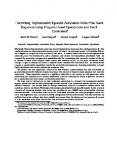
Steps 1 and 2 is performed early before the patterns are composed into rules by filtering and sorting generators and closed patterns. After the rules are generated, step 3 is performed. The rules are grouped into rule-groups. A rule group corresponds to a closed pattern and a set of generators related to it. There are 87 rule groups mined. After running the closed pattern mining algorithm, we found at least 5 interesting specifications corresponding to software behavioral patterns: C1 hConnection Set Up Evs, TxManager Set Up Evs, Transaction Set Up Evs, Transaction Commit Evs, Transaction Disposal Evsi C2 hConnection Set Up Evs, TxManager Set Up Evs, Transaction Set Up Evs, Transaction Rollback Evs, Transaction Disposal Evsi C3 hResource Enlistment Evs, Transaction Execution Evs, Transaction Commit Evs, Transaction Disposal Evsi C4 hResource Enlistment Evs, Transaction Execution Evs, Transaction Rollback Evs, Transaction Disposal Evsi C5 hLock-Unlock Evsi These patterns correspond to closed patterns of longest length and highest support. Note that the each “Evs” corresponds to a series of events. The longest pattern C1 is composed of 32 events. In addition to the closed patterns, with the mining of generators, we are also able to describe precondition events that underlie the long pattern hence forming a rule. Important minimal pre-condition events for each of the 5 patterns (Ci is paired with Gi) are as follows: G1 G2 G3 G4

hTxManager.Commiti hTransactionImpl.rollbackResourcesi hTransactionImpl.enlistResource, TxManager.Commiti hTransactionImpl.enlistResource,TransactionImpl.rollbackResourcesi G5 (a) hlocki and (b) hunlocki With these minimal pre-conditions, the mined specifications are more complete. Each of them is a rule stating what series of events happen after, before and in-between the minimal preconditions. For example, for the shortest rule involving lock and unlock, the rule group mined is able to say dually that: (1) when lock is acquired, lock must be released, (2) when lock is released, lock must be acquired before. Also, consider the longest rule mined. These are 5 minimal pre-conditions. These are marked with red dashed-boxes in Figure 11. Furthermore, since generators can be a combination of events, as are the cases with pre-conditions G3 and G4 above, mined specifications can describe the series of events that must happen in between the pre-condition’s constituent events. The specification rule(G4,C4) describes 24 other events that are bound to occur with likelihood more than 95% when two events enlistResource and rollbackResources are called. One of these events occurs before enlistResource, nine occur in between the two events, and 14 others occur after rollbackResources.

13

Connection Set Up 1. TransactionManagerLocator.getInstance 2. TransactionManagerLocator.locate 3. TransactionManagerLocator.tryJNDI 4. TransactionManagerLocator.usePrivateAPI Tx Manager Set Up 5. TxManager.begin 6. XidFactory.newXid 7. XidFactory.getNextId 8. XidImpl.getTrulyGlobalId Transaction Set Up 9. TransactionImpl.associateCurrentThread 10. TransactionImpl.getLocalId 11. XidImpl.getLocalId

Transaction Set Up (Con’t) 12. LocalId.hashCode 13. TransactionImpl.equals 14. TransactionImpl.getLocalIdValue 15. XidImpl.getLocalIdValue 16. TransactionImpl.getLocalIdValue 17. XidImpl.getLocalIdValue Transaction Commit 18. TxManager.commit 19. TransactionImpl.commit 20. TransactionImpl.beforePrepare 21. TransactionImpl.checkIntegrity 22. TransactionImpl.checkBeforeStatus

Transaction Commit (Con’t) 23. TransactionImpl.endResources 24. TransactionImpl.completeTransaction 25. TransactionImpl.cancelTimeout 26. TransactionImpl.doAfterCompletion 27. TransactionImpl.instanceDone Transaction Dispose 28. TxManager.releaseTransactionImpl 29. TransactionImpl.getLocalId 30. XidImpl.getLocalId 31. LocalId.hashCode 32. LocalId.equals

Fig. 11. Longest mined rule (32 events) from JBoss transaction component – read from top-to-bottom, left-to-right

8

D ISCUSSION

We discuss some issues and future work in the following paragraphs. Why a simple extension does not work? Closed iterative pattern mining algorithm proposed in [8] can not be trivially extended to mine for generators. To detect non-closed patterns, the algorithm in [8] tries to extend instances of P to form instances of a longer pattern P 0 . If all instances of P can be extended, then P is not closed. The approach works since, based on the apriori property, the longer pattern P 0 has less or equal instances as compared to P . One might be tempted to perform a similar approach to detect non-generators by removing events from instances of Q to form instances of a shorter pattern Q0 . Unfortunately, this does not work since shorter patterns can have more instances. Some of these instances might not correspond to any instance of the longer pattern. Similarly, the algorithm mining sequential generators in [15] can not be trivially extended to mine iterative generators since repetitions need to be addressed and the semantics of MSC/LSC need to be obeyed (which involves negation on the definition of pattern instance). A number of major properties of sequential patterns no longer apply to iterative patterns. First, the apriori property of sequential pattern is no longer true, i.e., it is not always the case that if a pattern P is a subsequence of another pattern P 0 , then sup(P ) ≥ sup(P 0 ). This is due to the negation involved in the definition of pattern instance following the semantics of MSC/LSC. Second, for sequential patterns, if two patterns P and P’ have the same projected database, i.e., DBP == DBP 0 , then any extension of P (P ++evs) will have the same projected database as the corresponding extension of P 0 (P 0 ++evs), i.e., DBP ++evs == DBP 0 ++evs . This property has been used in [15] to detect redundant search spaces. For iterative patterns, this is only true for approximate iterative patterns with approximated support. However our goal is still to mine iterative patterns with correct support. To do so, our approach first generates a compacted representation of approximate iterative patterns and then obtain iterative patterns with correct support from the compact representation of approximate iterative patterns. Third, the approach to detect equivalences of projected databases used in sequential pattern mining [21], [15] no longer applies in iterative pattern mining.

More details on this has been described previously in subsection 5.2. Also, the algorithm in [15] first generates many candidate patterns, many of which are not generators. After all the candidates have been produced, it then filters non-generators from the candidates. At times the number of candidate patterns to be compared could be too large. To address this we employ an efficient direct computation of iterative generators from a compact search space representation (i.e., PAL). Run-time and space complexity. In the worst case, the runtime complexities of mining iterative generators and mining closed patterns are the same as mining all frequent patterns. The latter is potentially exponential to the length of the longest sequence in the dataset. In the worst case, it is possible that all pruning strategies do not help in pruning any search space. However, in practice, pruning strategies could help greatly. To validate whether the pruning strategies help in practice, an extensive empirical study over 10 synthetic and 2 real datasets have been performed The space complexity of the algorithm is predominated with the space of storing the PAL data structure. In the worst case this space would be proportional to the number of frequent patterns. However, in practice this is much less due to the pruning of redundant search spaces. Handling minor errors in dataset. Software often contains bugs. We assume that a program is correct at most of the time and incorrect for a minority of the time. Since we consider the concept of confidence in the representative rules, we would be able to handle minor errors and faults because of their infrequent occurrences. Unimportant method calls. At times, there might be many unimportant events in the software traces, e.g., a call to getHashCode(), toString(), etc. These events could first be identified and removed from the dataset. These issues have been investigated by past issues [36], [37]. We could use their work as a pre-processing step to remove unimportant method calls. The filtered trace could then be the input to our approach. Non-overlapping pattern instances and nested patterns. In our study, patterns have non-overlapping instances3 . Including overlapping pattern instances could drastically increase the 3. This is the case except for patterns where a prefix of the pattern equals to a suffix, such as ha, b, ai. For these cases, there might be overlap but it does not cause a blow up in the number of reported pattern instances. For example, there are two instances of ha, b, ai in the trace: ha, b, a, b, ai.

14

support of a pattern inappropriately. Consider a single trace ha, a, a, b, b, b, c, c, ci, the support of ha, b, ci considering overlapping would be 33 = 27, while the support of hai is only 3. The semantics of iterative patterns is based on the standards in software modeling namely Message Sequence Charts and Live Sequence Charts. Nested patterns, e.g., hA, B, (C, D)∗, Ei in which (C, D)∗ corresponds to one or more occurrences of (C, D), are not mined at the moment. These correspond to capturing loop in a sequence diagram. However, even without nested patterns, the language is powerful enough to capture various forward-temporal specifications from many open source applications [27], [28]. In this study, we not only mine forwardtemporal, but also backward- and in-between- temporal specifications. The case study has shown the utility of the approach. We leave mining nested patterns as a future work.

9

C ONCLUSION

In this paper, we propose a novel algorithm to mine iterative generators as a step forward in developing data mining tools addressing the needs of software engineers. We also introduce a novel concept of representative rules expressing forward, backward and in-between temporal constraints. These rules characterize many real-world constraints including those found in software specifications and can be constructed by pairing iterative generators with closed iterative patterns. A comprehensive performance study and a case study have been conducted to evaluate the scalability and utility of the proposed approach. Acknowledgement. We wish to thank Blue Martini Software for contributing the KDD Cup 2000 data. We wish to thank the anonymous reviewers for their valuable comments. This work is supported in part by an A*STAR grant SERC 072 101 0016 and an NTU Tier-1 grant RG66/07.

R EFERENCES [1]

M. Lehman and L. Belady, Program Evolution - Processes of Software Change. Academic Press, 1985. [2] S. Deelstra, M. Sinnema, and J. Bosch, “Experiences in software product families: Problems and issues during product derivation,” in Proceedings of International Software Product Line Conference, 2004. [3] E. Erlikh, “Leveraging legacy system dollars for e-business.” IEEE IT Pro, pp. 17–23, 2000. [4] T. Standish, “An essay on software reuse.” IEEE Transaction on Software Engineering, vol. 10, pp. 494–497, 1984. [5] ITU-T, “ITU-T Recommendation Z.120: Message Sequence Chart (MSC),” 1999. [6] C. Steel, R. Nagappan, and R. Lai, Core Security Patterns. Sun Microsystem, 2006. [7] Java Transaction API (JTA), “http://java.sun.com/javaee/technologies/jta/ index.jsp (accessed 18 Dec 2008).” [8] D. Lo, S.-C. Khoo, and C. Liu, “Efficient mining of iterative patterns for software specification discovery.” in Proceedings of SIGKDD Conference on Knowledge Discovery and Data Mining, 2007. [9] R. Agrawal and R. Srikant, “Mining sequential patterns.” in Proceedings of IEEE International Conference on Data Engineering, 1995. [10] H. Mannila, H. Toivonen, and A. Verkamo, “Discovery of frequent episodes in event sequences,” Data Mining and Knowledge Discovery, vol. 1, pp. 259–289, 1997. [11] W. Damm and D. Harel, “LSCs: Breathing life into message sequence charts.” Formal Methods in System Design, vol. 19, pp. 45–80, 2001. [12] N. Pasquier, Y. Bastide, R. Taouil, and L. Lakhal, “Discovering frequent closed itemsets for association rules,” in Proceedings of Symposium on Principles of Database Systems, 1999.

[13] J. Li, H. Li, L. Wong, J. Pei, and G. Dong, “Minimum description length principle: Generators are preferable to closed patterns.” in Proceedigns of AAAI Conference on Artificial Intelligence, 2006. [14] J. Li, G. Liu, and L. Wong, “Mining statistically important equivalence classes and delta-discriminative emerging patterns.” in Proceedings of SIGKDD Conference on Knowledge Discovery and Data Mining, 2007. [15] D. Lo, S.-C. Khoo, and J. Li, “Mining and ranking generators of sequential rules,” in Proceedings of SIAM International Conference on Data Mining, 2008. [16] E. Clarke, O. Grumberg, and D. Peled, Model Checking. MIT Press, 1999. [17] M. Spiliopoulou, “Managing interesting rules in sequence mining.” in Proceedings of European Conference on Principles of Data Mining and Knowledge Discovery, 1999. [18] D. Lo, S.-C. Khoo, and C. Liu, “Efficient mining of recurrent rules from a sequence database.” in Proceedings of International Conference on Database Systems for Advanced Applications, 2008. [19] ——, “Mining past-time temporal rules from execution traces,” in Proceedings of International Workshop on Dynamic Analysis, 2008. [20] “MarkingQueuedIrps,” msdn.microsoft.com/enus/library/aa469118.aspx (accessed 18 Dec 2008). [21] X. Yan, J. Han, and R. Afhar, “CloSpan: Mining closed sequential patterns in large datasets.” in Proceedings of SIAM International Conference on Data Mining, 2003. [22] J. Wang and J. Han, “BIDE: Efficient mining of frequent closed sequences.” in Proceedings of IEEE International Conference on Data Engineering, 2004. [23] G. Garriga, “Discovering unbounded episodes in sequential data.” in Proceedings of European Conference on Principles of Data Mining and Knowledge Discovery, 2003. [24] M. Zhang, B. Kao, D. Cheung, and K. Yip, “Mining periodic patterns with gap requirement from sequences,” in Proceedings of SIGMOD International Conference on Management of Data, 2005. [25] B. Ding, D. Lo, J. Han, and S.-C. Khoo, “Efficient mining of closed repetitive gapped subsequences from a sequence database (to appear).” in Proceedings of IEEE International Conference on Data Engineering, 2009. [26] C. Gao, J. Wang, Y. He, and L. Zhou, “Efficient mining of frequent sequence generators,” in Proceedings of International Conference on World Wide Web (poster), 2008. [27] D. Lo, S. Maoz, and S.-C. Khoo, “Mining modal scenario-based specifications from execution traces of reactive systems,” in Proceedings of ACM/IEEE International Conference on Automated Software Engineering, 2007. [28] D. Lo and S. Maoz, “Mining scenario-based triggers and effects.” in Proceedings of ACM/IEEE International Conference on Automated Software Engineering, 2008. [29] D. Harel and R. Marelly, Come, Let’s Play: Scenario-Based Programming Using LSCs and the Play-Engine. Springer, 2003. [30] H. Kugler, D. Harel, A. Pnueli, Y. Lu, and Y. Bontemps, “Temporal logic for scenario-based specifications,” in Proceedings of International Conference on the Tools and Algorithms for the Construction and Analysis of Systems, 2005. [31] K. Olender and L. Osterweil, “Cecil: A sequencing constraint language for automatic static analysis generation.” IEEE Transaction on Software Engineering, vol. 16, pp. 268–280, 1990. [32] “Windows Driver Kit: Driver Development Tools – CancelSpinLock,” msdn.microsoft.com/en-us/library/aa469115.aspx (accessed 18 Dec 2008). [33] J. Pei, J. Han, B. Mortazavi-Asl, H. Pinto, Q. Chen, U. Dayal, and M.C. Hsu, “Prefixspan: Mining sequential patterns efficiently by prefixprojected pattern growth.” in Proceedings of IEEE International Conference on Data Engineering, 2001. [34] R. Kohavi, C. Brodley, B. Frasca, L. Mason, and Z. Zheng, “KDDCup 2000 organizers’ report: Peeling the onion,” SIGKDD Explorations, vol. 2, pp. 86–98, 2000. [35] M. Hutchins, H. Foster, T. Goradia, and T. Ostrand, “Experiments on the effectiveness of dataflow- and control-flow-based test adequacy criteria,” in Proceedings of International Conference on Software Engineering, 1994. [36] H. Zhong, L. Zhang, and H. Mei, “Early filtering of polluting method calls for mining temporal specifications.” in Proceedings of Asia-Pacific Software Engineering Conference, 2008. [37] A. Hamou-Lhadj and T. Lethbridge, “Summarizing the content of large traces to facilitate the understanding of the behaviour of a software system,” in Proceedings of IEEE International Conference on Program Comprehension, 2006.