Mining Message Sequence Graphs Sandeep Kumar† , Siau-Cheng Khoo† , Abhik Roychoudhury† , David Lo§ †
National University of Singapore
§
Singapore Management University
{sandeep,khoosc,abhik}@comp.nus.edu.sg
ABSTRACT Dynamic specification mining involves discovering software behavior from traces for the purpose of program comprehension and bug detection. However, mining program behavior from execution traces is difficult for concurrent/distributed programs. Specifically, the inherent partial order relationships among events occurring across processes pose a big challenge to specification mining. In this paper, we propose a framework for mining partial orders so as to understand concurrent program behavior. Our miner takes in a set of concurrent program traces, and produces a message sequence graph (MSG) to represent the concurrent program behavior. An MSG represents a graph where the nodes of the graph are partial orders, represented as Message Sequence Charts. Mining an MSG allows us to understand concurrent program behaviors since the nodes of the MSG depict important “phases” or “interaction snippets” involving several concurrently executing processes. To demonstrate the power of this technique, we conducted experiments on mining behaviors of several fairly complex distributed systems. We show that our miner can produce the corresponding MSGs with both high precision and recall.
Categories and Subject Descriptors D2.1 [Software Engineering]: Requirements / Specifications—Methodologies
General Terms Algorithms, Design, Experimentation
Keywords Specification Mining, Distributed Systems
1.
INTRODUCTION
Software is developed to cater to a specific set of requirements that are dictated by real life problems or business
Permission to make digital or hard copies of all or part of this work for personal or classroom use is granted without fee provided that copies are not made or distributed for profit or commercial advantage and that copies bear this notice and the full citation on the first page. To copy otherwise, to republish, to post on servers or to redistribute to lists, requires prior specific permission and/or a fee. ICSE ’11, May 21–28, 2011, Waikiki, Honolulu, HI, USA Copyright 2011 ACM 978-1-4503-0445-0/11/05 ...$10.00.
[email protected]
needs. However, a formal documentation of the software specification (the intended behaviors that the software is supposed to capture) is often missing, even though it is essential to the design, implementation and testing phases of software development. Moreover, formal software specifications are crucial for the maintenance of legacy software. As any software project team would agree, the cost for software maintenance is usually much higher than the initial software development cost. The cost of maintaining software and managing its evolution is said to account for more than 90% of the total cost of a software project, prompting certain authors to call it a “legacy crisis” [39]. The absence of any semi-formal and abstract representation in many development processes makes it difficult for users of the system to understand and appreciate its accurate behavior. In addition, several systems that follow recommended requirements gathering and design practises during early stages deviate from their early specifications as development and maintenance progresses. This deviation is a result of both errors in the implementation and changes in the requirements themselves. As a result, even if a software specification is available — it may not reflect the behaviors of the latest version of the program. Dynamic specification mining [11] is a dynamic program analysis method to automatically infer the specification of a program from its execution traces. The mining of various specification formats such as automata [11, 23, 28], and temporal rules [43, 25] has been studied. In general, specification mining techniques employ data mining or machine learning techniques on execution traces to generate models that are useful in program verification. However, these specification mining techniques have primarily been designed with sequential programs in mind. In order to apply such techniques on distributed systems the execution of each component has to be analyzed in isolation from rest of the system. In reality, the components of a distributed system do not function in isolation, but rather communicate and collaborate at several points of their execution. Very often, specifying how components interact becomes a crucial part of
Input Traces
MSG
Convert to Partial Order
Automaton Learning Identify Basic MSCs
Dependency Graphs
Mined Basic MSCs
Figure 1: Stages in the proposed mining framework.
(a)
Sample execution traces (inputs to our MSGMiner)
(b) Mined MSG (output from our MSGMiner) Figure 2: Banking System Example
the design of distributed system. In order to express such behavior, specification languages such as UML Sequence Diagrams or Message Sequence Charts (MSCs) are commonly used (e.g., see [14] for an early work on mining Sequence Diagrams). However, Sequence Diagrams only represent one scenario in the execution of a concurrent/distributed software — it does not capture the complete specification of the program’s behavior. In this paper, we study this problem. We propose MSGMiner - a framework to discover specifications of distributed systems as Message Sequence Graphs (MSGs). An MSG is a directed graph having an MSC at each of its vertices. These MSCs (referred to as basic MSCs ) only describe an interaction snippet in the system’s execution. Figure 1 describes the transformations performed by MSGMiner to construct an MSG. We convert each execution trace to a partial order (or dependency graph) by (i) considering the individual control flows across different processes and (ii) marking the dependencies between a send event and its corresponding receive. We then analyze these dependency graphs to find largest frequently recurring portions — which then appear as the basic MSCs in our mined model. The basic MSCs constitute the nodes of our mined MSG model. These nodes are then connected up using automata learning techniques. Our approach thus involves a combination of automata learning and mining of partial orders. Consider a hypothetical distributed banking system in which a user client interacts with a distant portal that in turn relies on a database at a separate location. Figure 2(a) shows three sample traces collected from executions of such a system. Figure 2(b) shows what an MSG mined from traces would appear like. The mined MSG is not an exact representation of the set of traces but instead a generalized model of the system suggesting many more possible scenarios. The main contribution of this paper is our framework for mining inter-process or inter-component concurrent system specifications in the form of a Message Sequence Graph (MSG). Conventional mining methods have focused on either intra-process specifications (where the control flow inside each process is mined as an automaton) or rule-based specifications (where system behavior is summarized as temporal properties either in textual form or in visual form such as Live Sequence Charts). It is worthwhile to emphasize that our focus on mining for MSGs involves a fundamental conceptual shift from mining of Live Sequence Charts (LSCs). This is because LSCs visually describe properties which must hold every system execution, whereas MSGs are a complete description of the global system behavior. Through the mined MSG model we emphasize the interaction snippets or commonly executed protocols across the processes and these get captured as the nodes or the basic MSCs in our mined MSG model. By understanding these
Figure 3: A schematic MSC and its partial order. frequently occurring interaction snippets, a programmer can understand the common concurrent interactions and in what sequence they occur — thereby getting a clear first-cut understanding of the behaviors of a concurrent program. We evaluated our MSG mining framework via case studies on real-life distributed software. It was found that the mining framework discovers MSG specifications that are easy to comprehend. Moreover, the mined MSG models compare favorably (in terms of precision/recall) w.r.t. manually constructed models.
2. BACKGROUND Message Sequence Charts (MSCs), a recommendation from ITU [4], have traditionally played an important role in software development and been incorporated into modelling languages such as ROOM [13], SDL [8] and UML [41]. The basic MSC syntax consists of a set of vertical lines-each denoting a process or a system component, internal events representing intraprocess execution and annotated uni-directional arrows denoting inter processes communication. Figure 3 shows a simple MSC with two processes; m1 and m2 are messages sent from p to q. Semantically, an MSC denotes a set of events (message send, message receive and internal events corresponding to computation) and prescribes a partial order over these events. This partial order is the transitive closure of (a) the total order of the events in each process1 and (b) the ordering imposed by the send-receive of each message.2 . It is also understood that arrows depicting the inter process communication is either a horizontal line or one that is slanting downwards. The events are described using the following notation. A send of message m from process p to process q is denoted as hp!q, mi. The receipt by process q of a message m sent by process p is denoted as hq?p, mi. Consider the chart in Figure 3. The total order for process p is hp!q, m1 i ≤ hp!q, m2 i where e1 ≤ e2 denotes that event e1 “happens-before” event e2 . Similarly for process q we have hq?p, m1 i ≤ hq?p, m2 i. For the messages we have hp!q, m1 i ≤ hq?p, m1 i and hp!q, m2 i ≤ hq?p, m2 i. The transitive closure of these four ordering relations defines the partial order of the chart. Note that it is not a total order since from the 1
Time flows from top to bottom in each process. The send event of a message must happen before its receive event. 2
transitive closure we cannot infer that hp!q, m2 i ≤ hq?p, m1 i or hq?p, m1 i ≤ hp!q, m2 i. Thus, in this example chart, the send of m2 and the receive of m1 can occur in any order. The partial order suggested by the MSC in this example is also shown in Figure 3. The vertical lines representing the independent processes or threads whose interactions we capture are also referred to as lifelines. MSCs can be formally defined as follows. Definition 2.1 (MSC). An MSC M can be viewed as a partially ordered set of events M = (L, {El }l∈L , ≤, γ, Σ), where L is the set of lifelines in m, El is the set of events in which lifeline l takes part in M . Σ is the alphabet of send and receive event labels and γ : {El }l∈L → Σ is a function assigning each send or receive event a label. ≤ is the partial order over the occurrences of events in {El }l∈L such that • ≤l is the linear ordering of events in El , which are ordered top-down along the lifeline l, • ≤sm is an ordering on message send/receive events in {El }l∈L . If γ(es ) = hp!q, mi and the corresponding receive event is er , withγ(er ) = hq?p, mi, we have es ≤sm er . S • ≤ is the transitive of ≤L = l∈L ≤l and ≤sm , S closure ⋆ that is, ≤= (≤L ≤sm )
Concatenation of MSGs can be defined in two different manners. For a concatenation of two MSCs say M1 ◦ M2 , all events in M1 must happen before any event in M2 . In other words, it is as if the participating processes synchronise or hand-shake at the end of an MSC. In MSC literature, it is popularly known as synchronous concatenation. On the other hand, asynchronous concatenation performs the concatenation at the level of lifelines (or processes). Thus, for a concatenation of two MSCs, say M1 ◦ M2 , any participating process (say Interface) must finish all its events in M1 prior to executing any event in M2 . For the rest of this paper we remain faithful to the latter definition of concatenation. An MSC of our definition is suited to specify a single execution scenario. A complete specification of a system would therefore require multiple MSCs. A large number of MSCs will be required to describe most non-trivial systems. For this reason, MSC standards include High Level Message Sequence Charts (HMSCs) that make it easy to define and visualize large collections of MSCs. HMSCs are hierarchical graphs that have as nodes either a basic MSC or a lower level HMSC chart. We limit our mining exercises to the simpler yet semantically equivalent representation of Message Sequence Graphs [21]. Formally an MSC-graph or MSG is a directed graph (V, E, Vs , Vf , λ), in which V is the set of vertices, E a set of edges, Vs a set of entry vertices, Vf a set of accepting vertices and λ a labelling function that assigns an MSC to every vertex. From any path in an MSG of the form (v1 , v2 . . . vn ), where v1 ∈ Vs ∧ vn ∈ Vf , we can derive one MSC by the concatenation of basic MSCs λ(v1 ) ◦ λ(v2 ) . . . λ(vn ).
3.
MINING ALGORITHM
MSGMiner takes in a collection of execution traces of a system implementation, and produces an MSG describing the system’s behavior. The main challenge in this process lies in the ability to discover occurrences of concurrency behavior from traces and specifying them using MSCs. We represent MSCs using data structures called dependency graphs
Figure 4: Dependency graphs for MSCs in Figure 2 that fully capture the partial order relationship among events in the MSC. Furthermore, we introduce a novel idea of maximal connected dependency graph (MCD) for a given trace set to capture basic MSCs that can be used as the building blocks for constructing an MSG. The entire mining process is thus divided into three stages, which are elaborated in the rest of the section: (1) Trace processing: Collection of traces and the transformation of each trace into a dependency graph. (2) MSC mining: Identifying basic MSCs (in MCD representation) from the dependency graphs, and transforming each dependency graph into a chain of MSCs. (3) MSG construction: Merging of chains of MSCs into an MSG.
3.1 Trace Processing and Dependency Graphs Traces are collected by instrumenting and executing a system implementation with various inputs. In a distributed system the trace points are chosen to be at program locations where processes send or receive messages. A trace event is either a send or receive message of the form hp ! q, mi or hq ? p, mi respectively, where m is the message being exchanged between a sender named p and a receiver named q. Furthermore every event must contain a time stamp to determine the ordering of events. For presentation clarity, we assume that traces are strings of events, which are drawn from a trace alphabet Σ. The collected traces record some linear temporal order in which events occur during the execution of the system. Our first task is to eliminate temporal ordering of events from different lifelines, when they are not explicitly imposed through messages. With these eliminations, we will have converted the total ordering of events implied by the traces into a partial ordering that captures concurrent behavior. Recall from 2.1 that an MSC M = (L, {El }l∈L , ≤, γ, Σ) prescribes the partial ordering ≤ among a set of events. ≤ was defined to be a transitive closure of the union of an ordering relationship between events within each lifeline(≤l ) and the ordering of send and receive events of a message (≤sm ). We observe that only the ordering imposed by ≤l and ≤sm are sufficient to specify the inherent behavior of the system, and define a dependency graph to capture these behaviors. Specifically, a dependency graph is a graph data structure g = (L, {Vl }l∈L , R, γ ′ , Σ) where: • each vi ∈ Vl corresponds to an event ei ∈ El , • there is a directed edge v1 Rv2 iff for their corresponding events e1 and e2 , (e1 , e2 ) ∈ (∪l∈L ≤l )∪ ≤sm • γ ′ (vi ) = γ(ei ) for every event ei and its corresponding vertex vi in the dependency graph.
We will use (V, R, γ) as a shorter representation for dependency graphs whenever the lifelines and event alphabet is not relevant to the analysis. Note that dependency graphs are a graphical representation equivalent to ‘traces’ in trace theory [17]. Figure 4 shows the corresponding dependency graphs g1 ,g2 ,g3 and g4 , for basic MSCs M1 , M2 , M3 and M4 respectively. Some of the properties of dependency graphs used by the mining algorithm are as follows. Definition 3.1 (Equivalence ≡). For dependency graphs g1 = (V1 , R1 , γ1 ) and g2 = (V2 , R2 , γ2 ), g1 ≡ g2 iff there exists a bijection f : V1 → V2 such that, ∀v1 ∈ V1 (γ1 (v1 ) = γ2 (f (v1 ))) and ∀v1 , v2 ∈ V1 (v1 R1 v2 ⇔ f (v1 )R2 f (v2 )).
used in graph theory. In Figure 5, gx , gy and gz are subgraphs of the concatenated dependency graph. The subgraph gx is a prefix and gz a suffix. Definition 3.5 (Frequency). The frequency of subgraph g ′ in dependency graph g is n, if there exist dependency graphs g0 , g1 , . . . gn such that g ≡ ((((g0 ◦g ′ )◦g1 )◦g ′ ) . . .)◦gn and g ′ * g0 , g1 . . . gn . Note that g0 , g1 . . . gn may be empty. Informally, the frequency of a sub-graph g ′ in g is the number of distinct occurrences of the g ′ in g. Figure 5 also shows the frequency of gx , gy and gz in (g1 ◦ g3 ) ◦ g2 .
Definition 3.2 (Concatenation ◦). For two graphs, g1 = (L1 , {V1l }l∈L1 , R1 , γ1 , Σ) and g2 = (L2 , {V2l }l∈L2 , R2 , γ2 , Σ) the concatenation g1 ◦ g2 = (L, {Vl }l∈L , R, γ, Σ) such that L = L1 ∪ L2 V1l ∪ V2l V1l Vl = V2l
if l ∈ L1 ∩ L2 if l ∈ L1 − L2 if l ∈ L2 − L1
γ = γ1 ∪ γ2 R = R1 ∪ R2 ∪ RL ∪ Rsr
The concatenated graph contains the following new sets of edges: 1. RL : This enforces the ordering that for a lifeline l, the events in V1l occur before those in V2l . Let function f irst(Vil ) return vertex v ∈ Vil such that ∀v ′ ∈ Vil , vRi v ′ . Similarly let l ast(Vil ) return the last event in lifeline l. RL = {(last(V1l ), first(V2l ))|∀l ∈ L1 ∩ L2 } 2. Rsr : This pairs an unmatched send event in g1 with an unmatched receive event in g2 . Since a graph may contain repetitions of the same send/receive event, we resolve ambiguity by defining a function ϕl : Vl → N0 to differentiate between identical events within the same lifeline. For a vertex v ∈ Vl , ϕl (v) = |{v ′ |v ′ ∈ Vl ∧ (v ′ , v) ∈ (RL ∪ R1 ∪ R2 )+ ∧ γ(v ′ ) = γ(v)}|. Rsr = {(vp , vq )|vp ∈ V1p ∧ vq ∈ V2q ∧ ∃ hp!q, mi, hq?p, mi ∈ Σ : γ(vp ) = hp!q, mi ∧ γ(vq ) = hq?p, mi ∧ ϕp (vp ) = ϕq (vq )} Figure 5 shows the result of concatenation of dependency graphs g1 , g3 and g2 of Figure 4. The dotted lines show newly added edges. Definition 3.3 (Sub-Graph). A sub-graph relationship among dependency graphs is as follows: g ′ ⊆ g if and only if there exist graphs x and y such that g ≡ (x ◦ g ′ ) ◦ y. Definition 3.4 (Prefix and Suffix). A sub-graph g ′ ⊆ g is a prefix of g iff for some graph y, g ≡ g ′ ◦ y. Similarly g ′ is a suffix iff for some graph x, g ≡ x ◦ g ′ . Our definition of sub-graph for dependency graphs is stricter than and not to be confused with the definition commonly
Figure 5: Concatenated graph (g1 ◦ g3 ) ◦ g2 , and some of its sub-graphs We define a function d graph(t) that accepts a trace t as parameter and constructs a dependency graph. The dependency graph is constructed by first creating a unique vertex for each occurrence of an event. After this, edges are added to link up events within a lifeline into a chain. Subsequently, the send and receive events are linked up in a backward fashion starting from the bottom of the trace. For example the last occurrence of event hq?p, mi is linked to the last occurrence of event hp!q, mi and so on. This manner of constructing a dependency graph gives function dgraph the property that given a trace t, for any of its suffixes ts , dgraph(ts ) is a suffix of dgraph(t). We have made two assumptions about the system during the construction: 1. No messages are lost in the message channels. 2. The message are sent over FIFO channels. The concatenated graph in Figure 5 is equivalent to dgraph (t1 ) constructed from trace t1 in Figure 2(a). The algorithm for function dgraph is detailed in a technical report [22].
3.2 MSC Mining Using the function dgraph, we convert the available trace set T = {t1 , t2 , . . . tn } to a set of dependency graphs G = {g1 , g2 , . . . gn }, where each dependency graph gi ∈ G corresponds to a scenario of system execution. Our next step is to identify basic sections within these graphs, that recur at several places within the same graph or across the graphs in G. These fundamental blocks are likely to capture the basic MSCs in an MSG describing the system. There are many possible ways to break down a graph into fundamental blocks. Our method aims to discover MSCs which are as big as possible and yet recurring frequently enough in the
input execution traces (or their corresponding dependency graphs). Therefore, we introduce the notion of Maximal Connected Dependency Graphs (MCDs) to signify MSCs. Formally, Definition 3.6 (MCD). For a given trace set T = {t1 , t2 , . . . tn }, gmcd = (V, R, γ) is an MCD iff 1. There is a trace t ∈ T such that gmcd ⊆ dgraph(t). 2. ∀g ⊂ gmcd : f req(gmcd ) = f req(g)
3
3. For every distinct v1 , v2 ∈ V , (v1 , v2 ) ∈ (R ∪ R−1 )∗ . 4. There is no graph g ′ that satisfies conditions 1-3 such that gmcd ⊂ g ′ . Criterion 2 guarantees that no part of an MCD (and thus its corresponding MSC) appears in some context in which the rest of the MCD does not also appear. Criterion 4 enforces the maximality of MSCs. Criterion 3 requires that events in MCDs be connected with each other. This additional constraint is introduced to simplify the mining task. An exhaustive search for graph structures that meet the conditions specified above could turn out to be expensive. Instead, we identify a graph structure termed event tail for each event, and then successively merge them to arrive at dependency graphs that will satisfy the frequency, connectedness and maximality criteria of MCDs. We describe event tails and the method of merging graphs in the following subsections.
3.2.1 Event Tail For an event e ∈ Σ, when given a trace set T ⊆ Σ∗ , its tail, tail[e], is the largest dependency graph that contains a single minimal vertex (which is a vertex in the graph without any associated incident edges) labelled e and satisfies conditions 1-3 of definition 3.6. Apart from the minimal vertex, it also contains all events that immediately follows every occurrence of e in a consistent partial order. Algorithm 1 outputs an associative array - tail, that maps every event in Σ to its tail. For an event e and trace set T , Te is the set of trace suffixes that start with e. Te can be easily derived from a suffix tree[40] constructed from the trace set. From Te we obtain a collection of suffix graphs, by identifying d graph(ts ) for every ts ∈ Te . In such a graph, let ve be the vertex corresponding to the first occurrence of event e. All vertices v in the graph for which (ve , v) 6∈ R∗ are removed as they do not belong to the tail. After this, the function getCommonPrefix is invoked to identify the largest prefix common to all suffix graphs in the collection for event e. This common prefix is the desired event tail tail[e]. Operationally, function getCommonPrefix identifies the largest common prefix in a pair of dependency graphs g1 and g2 through a simultaneous breadth-first traversal over these two graphs. During the traversal, vertices and edges are gradually added to the largest common prefix g. A vertex v with label e is added to g if and only if 1) there are vertices v1 in g1 and v2 in g2 having a common label e, and 2) v1 and v2 have identical incident edges and all vertices from which there are edges incident to v1 , v2 have already been added to g. In addition, getCommonPrefix ensures that all events added to the common graph have identical frequencies. All these operations ensure that conditions 1,2 and 3 of 3 Given a trace set T = {t1 , t2 , . . . tn }, freq(g) is the sum of the frequency of g in dgraph(t1 ), dgraph(t2 ), .. dgraph(tn ).
Algorithm 1 Find Event Tails Input: T - The trace set, Σ - set of events appearing in T . Output: tail[e] that maps every event e ∈ Σ to its tail. 1: for all e ∈ Σ do 2: Find Te : the set of all suffixes(of traces in T ) starting with e 3: let Te = {ts1 , ts2 , . . . tsne } 4: tail[e] ← ∅ 5: for i = 1 . . . ne do 6: (V, R, γ) ← dgraph(tsi ) 7: let ve be the vertex corresponding to the first event e 8: for all v ∈ V s.t. (ve , v) ∈ / R∗ do 9: V ← V − {v} 10: end for 11: if tail[e] = ∅ then 12: tail[e] ← (V, R, γ) 13: else 14: tail[e] ← getCommonPrefix(tail[e] , (V, R, γ)) 15: end if 16: end for 17: end for
definition 3.6 are satisfied. Moreover, since the event tail is the maximal graph common to all suffixes with ve as its minimal vertex, we have ensured that 1) tail[e] contains atleast one vertex ve , and 2) tail[e] cannot be extended without violating conditions 1,2 or 3. Details of getCommonPrefix is presented in [22]. Figure 6(a) shows some of the event tails derived from traces of the banking system in Figure 2.
3.2.2 Combining Event Tails Algorithm 2 uses the mapping from events to tails (tail[e]) to derive a mapping from events to MCDs - M CD[e]. The algorithm starts with g1 = tail[e]. We know that tail e cannot be extended at the end as it is already maximal. Hence we attempt to grow g1 by prefixing it with other graphs. For every event e′ we verify if tail[e′ ] can be merged into g1 . Let tail[e′ ] be the graph g2 . Without loss of generality we can express the two tails as, g1 ≡ g1pref ◦ g comm and g2 ≡ (g2pref ◦ g comm ) ◦ g2suff where g comm is the largest possible such graph. If g comm is empty, we do not perform any merging. If g comm is not empty, we obtain g2pref ◦ g1 as the merged graph. To satisfy the frequency criterion, we chose to accept the merged graph only when freq(g2pref ◦g1 ) = freq(g1 ). When more than one prefix of g2 satisfy the conditions on g2pref , we select the largest one. The dependency graph g1 is an MCD if no more event tails can be merged into it. [22] provides a proof for the claim that for each event e1 , M CD[e1 ] determined by Algorithm 2 is an MCD. Figure 6(b) shows the set of MCDs that are obtained by merging event tails obtained from traces in Figure 6(a).
3.2.3 Converting Trace to Sequence of MSCs Algorithm 2 associates each event with an MCD. Utilizing this association, we transform every trace from the given trace set into a sequence of dependency graphs. To achieve this, we group events in a trace based on their associated MCDs. For a trace t, we represent each group of events by a dependency graph gi and derive a sequence of the form (g1 , g2 , . . . gi . . . gm ) such that d graph(t) ≡ ((g1 ◦ g2 ) . . .) ◦ gm . The order of dependency graphs in the sequence is constrained by the dependency relationship between events in d graph(t). In most cases, we can expect gi to be one of the MCDs we identified. Certain cases warrant special handling. Firstly,
(a)
(b)
Figure 6: (a)Event tails and (b)MCDs for events in the traces of the banking system Algorithm 2 Combine Event Tails
Algorithm 3 Convert to full MSCs
Input: tail[e] for all events e ∈ Σ Output: M CD[e] for all events e ∈ Σ 1: for all e1 ∈ Σ do 2: W ← Σ − {e1 } 3: g1 ← tail[e1 ] 4: while ∃e2 ∈ W s.t. merge(g1 , tail[e2 ]) 6= ǫ do 5: g1 ← merge(g1 , tail[e2 ]) 6: W ← W − {e2 } 7: end while 8: MCD[e1 ] ← g1 9: end for
Input: gList - A sequence of dependency graphs Output: outputList - Sequence of dependency graphs, each representing a valid MSC 1: outputList ← [ ] 2: temp ← gList[0] 3: for i ← 1 . . . gList.size() do 4: if temp has an unmatched send event then 5: temp ← temp ◦ gList[i] 6: else 7: outputList.add(temp) 8: temp ← gList[i] 9: end if 10: end for 11: return outputList
merge(g1 , g2 ) Input: g1 , g2 - The candidates for merging Output: The merged graph. (ǫ if merge is not possible). 1: Let gcomm be the largest suffix of g1 that is a sub-graph of g2 . 2: if (gcomm is empty) then 3: return ǫ 4: else 5: Find largest g2pref that satisfies: g2 ≡ (g2pref ◦ gcomm ) ◦ g2suff ∧ freq(g2pref ◦ g1 ) = freq(g1 ) 6: if no such g2pref is found then 7: return ǫ 8: else 9: return g2pref ◦ g1 10: end if 11: end if
we may have derived two MCDs that share a common sub graph. For example, we may have M CD[e1 ] ≡ gx ◦ g and M CD[e2 ] ≡ g ◦ gy . Since MCDs are maximal, we know that the merged graph (gx ◦ g) ◦ gy must have a lower frequency that its sub graphs. In such scenarios, we will drop the common sub graph g from one of the MCDs. Secondly, two MCDs may not co-exist as they constrain each other in certain traces. To resolve such cases, we automatically split one of the MCDs into smaller parts whenever necessary. This scenario is explained with an example in [22]. While we have defined MCDs as dependency graphs, we do not require them to correspond to ‘complete MSCs’; ie., there may exist a send event in an MCD which does not contain the matching receive event and vice versa. In order to guarantee that all vertices of an MSG denote complete MSCs, we concatenate successive partial graphs in a postprocessing step to ensure that each dependency graph in the final sequence of MSCs will represent a complete MSC. Algorithm 3 performs this transformation. It takes a sequence of dependency graph gList and creates outputList - a list of dependency graphs without any unmatched send or receive events. At the end of this stage we have defined an alphabet of basic MSCs and produced strings from this alphabet for the construction of MSGs.
3.3 Constructing Message Sequence Graphs There exists a choice of algorithms to learn a finite state machine (FSM) from a training set of strings [12, 15]. For our experiments we implement a variant of the sk-strings algorithm as described in [35]. A shared prefix tree is initially constructed from the set of MSC strings. The algorithm then identifies a set of nodes that are equivalent. Two nodes are considered equivalent if their k-futures match. The k-future of a node is simply the set of all valid paths of length k or less (if the end node is reached) starting from that node. Several possible heuristics have been suggested to match two sets of k-futures. For better precision one could insist on the match being exact. Other methods involve matching two sets of strings if they meet a certain probabilistic threshold. Equivalent nodes are merged to get a more general and compact model. During the merging process loops are introduced to the model. For a prefix tree with n nodes, since every pair of nodes are compared, the algorithm has a worse case execution time of O(n2 mk ), where m is the size of the trace alphabet. For an operation comparing the k-futures of any two nodes, the maximum number of nodes to be compared is never greater than the total number of nodes in the tree. As a result, the algorithm has an execution time not worse than O(n3 ) for any value k. Note that n is shorter than the number of events in the initial traces as we have transformed them to MSC strings. Once an MSG has been mined from traces using the FSM learner, it is refined through a series of state reduction steps. An FSM learner usually produces a Mealy model state machine which in our setting has to be transformed into a minimal Moore model. In the latter state machine each state corresponds to a basic MSC. The final MSG is a structurepreserving homeomorphic embedding of the Moore model state machine. The general rule for reduction is that if any
state s is reachable from one and only one state s’ and s is the only state reachable from state s’, then the MSC in state s can be concatenated to the MSC in state s’. This concatenation yields new basic MSCs. The reduced directed graph of basic MSCs is our final output. The MSG can be exported as image files for visualization.
3.4 Extensions Our work on MSG Mining has relied on a simple definition of MSCs which was sufficient to represent partial order arising from asynchronous message exchanges. This constraints us from representing more complicated behavior within MSCs. For example, in some systems, a process may broadcast messages to multiple processes and await responses from its audience. We refer to such instances as “message broadcasts”. In such scenarios, the order in which the messages are sent or the responses received is usually inconsequential. Furthermore, the actual order of events seen in traces may be different for each realization of such broadcasts. Without knowledge of “message broadcasts”, the mining process presented thus far may fail to produce a succinct and comprehensible MSG. MSG semantics [4] provide features such as coregions or par inline expressions to capture situations where there may be no specific logical ordering between some events within a lifeline. The par expression allow us to list a group of MSCs and imply that they are to be executed in parallel. To handle such scenarios using these features, we extend the existing framework to accept additional input that declares specific behaviour, such as the presence of broadcast messages. We term this additional input an oracle. Our extended system when informed by the oracle, will construct customized dependency graphs and identify MCDs that capture such scenarios; the MSGs produced by the extended system become less cluttered and much more comprehensible. The technical report [22] details the use of such oracles to extend the system.
4.
CASE STUDIES
Through case studies, we attempt to evaluate the practicality of employing MSGMiner on real distributed systems. In each case, we have also scored the accuracy of mining by comparing the MSGs mined from traces to hand derived specifications. We consider the following distributed systems: (a) “Center TRACON Automation System” [31] an air traffic control system from NASA, (b) a system of server and VOiP clients communicating based on the Session Initiation Protocol (SIP) and (c) a system of Server and Clients that follow the XMPP Instant messaging and Chat protocol. In each of these systems, multiple processes perform asynchronous communication over TCP socket connections. Timestamped traces were collected by inserting instrumentation code at points were messages are written to or read from a socket. The traces were filtered and the message names abstracted with the help of text processing scripts.
4.1 Evaluation We propose an evaluation technique to validate the mined model against a known correct model. The correct model is used only for evaluation and never part of the mining process. Given correct and mined models, we derive a precision and recall score by performing language comparison. Precision and recall are popular metrics in Information Retrieval
and have also been used to quantify the accuracy of mined state based models [23, 29]. Recall that concatenating basic MSCs along any path from a starting vertex to an accepting vertex in the MSG produces an MSC that represents a valid execution scenario. We say that such an MSC is ‘generated’ by the MSG. Precision is defined as the number of MSCs generated by the mined model that are accepted by the correct model divided by the total number of MSCs generated by the mined model. Similarly recall is the ratio of the number of MSCs from the correct model that are accepted by the mined model to the total number of MSCs generated by the correct model. All possible MSGs can not be enumerated as infinitely many MSCs can be generated from an MSG. Instead we use only a finite sample from the MSG’s language for evaluation. Our sample consists of all accepting paths in the MSG with a finite bound on loops. This bound is enforced my limiting the number of times any vertex is revisited in a path. For the dependency graph g corresponding to each MSC from the generating MSG, we verify if there is a path in the accepting MSG that forms a dependency graph identical to g. This is done by an efficient depth first search in the accepting graph. As our case studies consider reactive systems that contain concurrently executing processes, existing automaton learning methods can not be applied to their traces. Such methods can instead be used to infer a state machine for each process if the original traces are separated into traces local to each of the constituent processes. We compare the accuracy of our proposed approach with the accuracy of mining this alternative model of local automata from the same collection of traces. To do this, we derive a similar precision and recall score of the learnt automata with respect to the same correct MSG specification that was used to score the mined MSG. The algorithm used to learn automata is identical to the method used in the automaton learning phase of MSG mining (Section 3.3). Precision and recall for automata is measured as the ratio of the number of traces(rather than MSCs) generated from one model that is accepted by the other model to the total number of traces generated. We generate random sample of traces from the collection of automata. The parallel composition of the automata may contain accepting paths that create invalid traces(eg: Receive event may appear before the message is sent). To generate only ‘correct’ traces we simulate the FIFO message channels between processes. While exploring a path in the composed automaton, if an edge outputting a send event hp!q, mi is chosen, the message m placed in the buffer corresponding to the channel [p → q]. An edge outputting a receive event hq?p, mi can be explored only if message m can be removed from the front of buffer [p → q]. A path explored in the composed automaton signifies a valid trace only when an accepting state is reached and all the message buffers are empty. We impose a bound on the number of loops as before. Table 1 tabulates the results from the case studies. It shows the precision, recall and F1 measure(harmonic mean of precision and recall) of the mined models obtained from the two alternatives (automaton learning and MSG Mining) for each case study. The mining was performed on a JVM running on an Intel duo core CPU with 1GB of available memory. The results from the systems considered for case study suggest that the proposed MSG mining method provides better mining accuracy.
System SIP XMPP-Core XMPP-MUC CTAS
No of events 1870 3212 5736 6418
Prec 0.50 0.72 1 0.95
Mined Automata Rec F1 Score 1 0.67 0.44 0.55 1 1 1 0.97
Time(s) 1.0 8.3 22.0 48.1
Prec 0.78 1 1 1
Mined MSG Rec F1 Score 0.87 0.82 0.71 0.83 1 1 1 1
Time(s) 3.14 10.2 28.7 45.8
Table 1: Table comparing accuracy of mining for MSG and Automata specifications
4.2 CTAS CTAS is an Air Traffic Control system from NASA. The CTAS weather control logic specification [32] was one of the case studies recommended by the 3rd International Workshop on Scenarios and State Machines (SCESM04). CTAS is a distributed system having a central Communications Manager (CM) process to which client processes connect. The weather control specification details how clients should connect to CM and how a graphical user interface referred to as the weather control panel (WCP) ought to communicate with CM to update weather status. As access to the CTAS system is limited, we procure execution traces by implementing and executing a simulation of this system in Java. Our implementation is based on a formal specification of the system in Promela and high level HMSC that was developed by a fellow researcher. The MSG mined from the collected traces is shown in Figure 7. Our mining on the CTAS system succeeds in identifying the states of the system that are mentioned in the informal requirements documents. The narrative in sub-sections of the document matches neatly with the visual representation provided by the basic MSCs.
4.3 Session Initiation Protocol SIP is a signalling protocol used to establish, manage and terminate VoIP calls and multimedia sessions in general [7]. SIP clients interact with servers that perform the necessary call routing and function as gateways to the Public Switched Telephone Network(PSTN). We attempt to specify how clients should interact with their proxy server to achieve some of the basic call features. For this, we set up a system having three SIP clients connected to a single server. We use instrumented versions of KPhone [3] - a SIP client implementation and the Opensips server [5] both of which are available with source code under a GPL license. We execute a set of test cases involving features such as basic call setup, call screening and call forwarding. A set of test cases for each feature are identified and a trace set is prepared by executing them on the system. The test cases involve three clients or SIP user agents labelled as Alice, Bob and Carol whose roles were restricted in the following way. In all test cases, Alice initiates calls and Bob is the intended recipient. Features such as call screening or forwarding are enabled at the client Bob. Carol is the recipient of diverted calls. Specification mining was performed from the trace set. A specification(that reflects allotted client names and roles) was manually derived by the authors for quantitative analysis and comparison.
4.4 XMPP Extensible Message and Presence Protocol is an open Instant Messaging standard originally developed by the Jabber open source community. The core functionality of the protocol is specified in rfcs 3920 and 3921. XMPP is the protocol for exchange of instant chat messages and presence information between various entities in a network that are addressed
by unique jabber ID. The clients communicate to the server through structured XML messages. The protocol defines how XML nodes known as stanzas are to be exchanged between various entities. A client connecting to a server is authenticated through TLS or SASL through special XML stanzas. We attempt to discover the client server interaction protocol from a system having two jabber clients that are brokered by a single server. In the specification, the server and client processes are the lifelines and the message arrows represent the XML stanzas. The Openfire XMPP server [2] and Jeti [1]/Pidgin [6] client implementations were instrumented and executed for trace collection. For discovering the core specification as an MSG, we only record stanzas used for authentication or those having a message or presence tag and ignore rest of the message exchanges. In addition to the core specification, XMPP Standards Foundation (XSF) has standardised several additional chat features. We attempt to mine behavioral specification for the Multi User Chat(MUC) functionality [9]. For this we use a separate set of test cases involving features such as service discovery, multi-party chat and creation and administration chat rooms. In all test cases user1 creates the chat room thereby acquiring the role of the room owner. Only messages sent from or addressed to the MUC conference service are recorded.
5. RELATED WORK Research in specification mining has attempted to discover common specification formats like frequent patterns & rules [24, 38, 10, 43, 25], finite state machines [11, 23, 28, 30, 16, 42, 34, 20, 10] and Boolean expressions [19]. Approaches that mine frequent patterns highlight statistically significant patterns in the execution of the system which can be interpreted as temporal rules. While the mined set of rules and properties are valuable to processes like model checking, they provide a limited understanding of the system as a whole. We mine for MCDs based on a frequency criterion and use them along with automaton learning methods to provide a complete sepcification of the system. Most methods that mine finite state machines are built upon the k-tails learner [12]. In mined state machines, the transition edges between program states are usually labelled with method calls. Ammons et al. propose the use of automaton mining on execution traces to infer state machine specifications for Application Programming Interfaces (API) [11]. The precision and recall of automaton mining is improved by a trace filtering and clustering method proposed by Lo and Khoo [23]. Lorenzoli et al. further combines the work of Daikon[19] with mining finite state models [28]. Boolean invariants are attached to transitions among the nodes in the finite state machines to express guards. Our approach uses a similar automaton mining algorithm, but performs additional steps so as to mine state machines having MSCs at each node. It is possible to apply the techniques proposed in the past work on top of our method to improve the mining accuracy (e.g., by performing trace
Figure 7: The Mined MSG for CTAS (left) and the learnt automata for individual processes filtering and clustering) and enhance the expressiveness of the mined model (e.g., by the addition of guards). In [10], Archaya et al. extract relevent API interaction scenarios out of static traces generated from program code. The scenarios are then summarized as compacted partial orders. A collection of work that attempts to infer frequent partial order from string databases is discussed in [18]. The generic partial order representation that is identified can be used to explain multiple sequences occuring in the database. Lou et al. in [29] construct workflow models from traces of concurrent systems by identifying dependency relationships between pairs of events in interleaved traces. Different from the above studies, we express partial orders in the semantics of Message Sequence Charts (MSCs). MSC is a popular specification language and formally specifies the partial order constraints among messages sent between lifelines. Also, we compose many partial orders into a message sequence graph (MSG). The work of [27, 26] mine Live Sequence Charts (LSC) that represent rules of the format “If the execution described by the pre-chart occurs, the execution prescribed by the main chart must eventually follow”. We emphasize that our focus on mining for MSGs (a global system model) involves a fundamental conceptual shift from mining of LSCs (a collection of temporal properties). This is because LSCs are simply a visual description of temporal properties which must hold in every system execution. In contrast, MSGs are a complete description of the global system behavior. Through the mined MSG model we highlight the interaction snippets or commonly executed protocols across the processes and these get captured as the nodes or the basic MSCs in our mined MSG model. Efforts have been made in program visualization by constructing UML sequence diagrams from dynamic executions [14, 33]. Such work constructs a sequence diagram from dynamic traces traces but does not produce graph-based models like MSG that include loops and branches. Rountev et. al. [36], perform a static inter-procedural analysis to reverse engineer UML Sequence Diagrams from programs. Such an analysis requires the program source code, whereas our analysis, being dynamic, only needs execution traces. We also present a framework that supports mining with synchronous/asynchronous message passing(within MSCs) and
synchronous/asynchronous concatenation(across MSCs) — making it a fully general framework for mining MSC-based system models.
6. CONCLUSION AND FUTURE WORK In this paper, we have presented a dynamic specification mining framework to mine Message Sequence Graphs from execution traces of concurrent/distributed programs. Our focus on Message Sequence Graphs is driven by the view that the mined specification will be used for program comprehension. Thus, our mining framework exploits the easeof-use of MSCs/MSGs for understanding interactions in a concurrent/distributed software. As demonstrated by our experiments, an MSG being a global graph of interaction snippets — provides a higher-level view of the system behavior (and its interactions), as compared to mining the behavior of individual processes of a concurrent program as state machines. In future, we plan to pursue several avenues to extend the work. One particular issue relates to the succinctness of mined MSGs. We observe that many large scale concurrent/distributed programs are essentially parameterized systems containing several processes which are behaviorally “similar”. For instance, multiple clients in the chat system perform many similar actions such as login and sign out. This can result in several redundant basic MSCs in the MSG, that try to explain the same behavior. One way to manage such complexity would be to automatically identify such similar basic MSCs during the mining process, and group them together. This requires us to develop a formal notion of “roles” and attach distinct roles to the participating processes in an MSC (e.g. see [37] for ideas along these lines). Mining MSC-based system models for large-scale parameterized distributed software in such a fashion remains an important direction of our future research. In a broader perspective, our work can be seen as a precursor of a multiview mining framework, in which multiple views of a system model are mined from the execution traces. In particular, we envision a mining framework which mines state-based intra-process style specifications as well as MSC-based interprocess style specifications from the traces of a concurrent / distributed system.
7.
ACKNOWLEDGEMENT
This work was partially supported by NUS research grants R-252-000-385-112 and R-252-000-403-112.
8.
REFERENCES
[1] Jeti. Version 0.7.6 (Oct. 2006). //jeti.sourceforge.net/. [2] Jive software. //www.igniterealtime.org/projects/openfire/. [3] KPhone. //sourceforge.net/projects/kphone. [4] Message sequence charts. ITU-TS Recommendation Z.120, 1996. [5] Opensips. //www.opensips.org/. [6] Pidgin. //www.pidgin.im/. [7] RFC 3261 - Session Inititation Protocol. //www.ietf.org/rfc/rfc3261.txt/. [8] Specification and description language. ITU-T Recommendation Z.100. [9] XEP-0045:Multi-User Chat. http://xmpp.org/extensions/xep-0045.html. [10] M. Acharya, T. Xie, J. Pei, and J. Xu. Mining API patterns as partial orders from source code: from usage scenarios to specifications. In ESEC/SIGSOFT FSE, 2007. [11] G. Ammons, R. Bodik, and J. R. Larus. Mining Specification. In POPL, 2002. [12] A. Biermann and J. Feldman. On the synthesis of finite-state machines from samples of their behaviour. IEEE TOC, 21:591–597, 1972. [13] G. G. Bran Selic and P. T. Ward. Real-Time Object-Oriented Modeling. John Wiley & Sons, Inc., 1994. [14] L. C. Briand, Y. Labiche, and J. Leduc. Toward the Reverse Engineering of UML Sequence Diagrams for Distributed Java Software. IEEE TSE, 32(9):642–663, 2006. [15] J. E. Cook and A. L. Wolf. Discovering models of software processes from event-based data. TOSEM, 7(3), 1998. [16] V. Dallmeier, C. Lindig, A. Wasylkowski, and A. Zeller. Mining Object Behavior with ADABU. In WODA, 2006. [17] V. Diekert. The Book of Traces. World Scientific Publishing Co., Inc., River Edge, NJ, USA, 1995. [18] G. Dong and J. Pei. Mining partial orders from sequences. In Sequence Data Mining, volume 33 of Advances in Database Systems, pages 89–112. Springer US, 2007. [19] M. Ernst, J. Cockrell, W. Griswold, and D. Notkin. Dynamically Discovering Likely Program Invariants to Support Program Evolution. IEEE TSE, 27(2):99–123, 2001. [20] M. Gabel and Z. Su. Online inference and enforcement of temporal properties. In ICSE, pages 15–24, 2010. [21] J. G. Henriksen, M. Mukund, K. N. Kumar, and P. S. Thiagarajan. On message sequence graphs and finitely generated regular msc languages. ICALP ’00. [22] S. Kumar, A. Roychoudhury, S.-C. Khoo, and D. Lo. Mining message sequence graphs (technical report). www.comp.nus.edu.sg/∼sandeep/msgmining TR.pdf, 2010.
[23] D. Lo and S.-C. Khoo. SMArTIC: Towards building an accurate, robust and scalable specification miner. In SIGSOFT FSE, 2006. [24] D. Lo, S.-C. Khoo, and C. Liu. Efficient mining of iterative patterns for software specification discovery. KDD, 2007. [25] D. Lo, S.-C. Khoo, and C. Liu. Mining temporal rules for software maintenance. JSME, 20(4):227–247, 2008. [26] D. Lo and S. Maoz. Mining Scenario Based Triggers and Effects. In ASE, 2008. [27] D. Lo, S. Maoz, and S.-C. Khoo. Mining Modal Scenario-Based Specifications from Execution Traces of Reactive Systems. In ASE, 2007. [28] D. Lorenzoli, L. Mariani, and M. Pezz`e. Automatic Generation of Software Behavioral Models. In ICSE, 2008. [29] J.-G. Lou, Q. Fu, S. Yang, J. Li, and B. Wu. Mining program workflow from interleaved traces. In KDD, 2010. [30] L. Mariani and M. Pezz` e. Behavior capture and test: Automated analysis for component integration. In ICECCS, 2005. [31] NASA. Center TRACON Automation System (CTAS). //www.aviationsystemsdivision.arc.nasa.gov/ research/foundations/sw overview.shtml. [32] NASA. CTAS Weather Control Requirements. //scesm04.upb.de/case-study-2/requirements.pdf. [33] R. Oechsle and T. Schmitt. Javavis: Automatic program visualization with object and sequence diagrams using the java debug interface (jdi). In Revised Lectures on Software Visualization, International Seminar, pages 176–190, 2002. [34] M. Pradel and T. R. Gross. Automatic generation of object usage specifications from large method traces. In ASE, 2009. [35] A. V. Raman and J. D. Patrick. The sk-strings method for inferring PFSA. In Proc. of the workshop on automata induction, grammatical inference and language acquisition, 1997. [36] A. Rountev and B. Connell. Object naming analysis for reverse-engineered sequence diagrams. In ICSE, 2005. [37] A. Roychoudhury, A. Goel, and B. Sengupta. Symbolic message sequence charts. In ESEC-FSE, 2007. [38] H. Safyallah and K. Sartipi. Dynamic Analysis of Software Systems using Execution Pattern Mining. In ICPC, 2006. [39] R. Seacord, D. Plakosh, and G. Lewis. Modernizing Legacy Systems: Software Technologies, Engineering Processes, and Business Practices. Addison-Wesley, 2003. [40] E. Ukkonen. On-line construction of suffix-trees. Algorithmica 14, pages 249–260, 1995. [41] UML. The Unified Modeling Language. Available from //www.omg.org. [42] N. Walkinshaw, K. Bogdanov, M. Holcombe, and S. Salahuddin. Reverse engineering state machines by interactive grammar inference. In WCRE, 2007. [43] J. Yang, D. Evans, D. Bhardwaj, T. Bhat, and M.Das. Perracotta: Mining temporal API rules from imperfect traces. In ICSE, 2006.