Mining Multiple Level Non-redundant Association

Mining Multiple Level Non-redundant Association Rules through Two-Fold Pruning of Redundancies Corrado Loglisci and Donato Malerba Dipartimento di Informatica Universita’ degli Studi di Bari Via Orabona 4, 70125, Bari - Italy {loglisci,malerba}@di.uniba.it

Abstract. Association rules (AR) are a class of patterns which describe regularities in a set of transactions. When items of transactions are organized in a taxonomy, AR can be associated with a level of the taxonomy since they contain only items at that level. A drawback of multiple level AR mining is represented by the generation of redundant rules which do not add further information to that expressed by other rules. In this paper, a method for the discovery of non-redundant multiple level AR is proposed. It follows the usual two-stepped procedure for AR mining and it prunes redundancies in each step. In the first step, redundancies are removed by resorting to the notion of multiple level closed frequent itemsets, while in the second step, pruning is based on an extension of the notion of minimal rules. The proposed technique has been applied to a real case of analysis of textual data. An empirical comparison with the Apriori algorithm proves the advantages of the proposed method in terms of both time-performance and redundancy reduction. Keywords: Association Rules, Multiple Level Rules, Redundant Information.

1

Introduction

Association rules are a class of patterns which describe regularities or co-occurrence relationships in a set of data (e.g., transactions) [1]. Formally, an association rule is expressed in form of A⇒C, where both the antecedent A and the consequent C are sets of items (or itemsets) such that A∩C =. The meaning of an association rule is quite intuitive: a transaction which contains A is likely to contain C as well. To quantify this likelihood, two statistical parameters are usually used, namely support and confidence. The former, denoted as s(A ⇒ C), indicates the portion of the transactions where the conjunction A∪C occurs, and hence estimates the probability P(A∪C). The latter, denoted as c(A ⇒ C), indicates the portion of the transactions where C occurs out of the transactions in which A is present, thus it estimates the posterior probability P(C|A). The problem of association P. Perner (Ed.): MLDM 2009, LNAI 5632, pp. 251–265, 2009. c Springer-Verlag Berlin Heidelberg 2009 

252

C. Loglisci and D. Malerba

rule mining consists of finding out all rules whose support and confidence values exceed two user-defined thresholds, called minsup and minconf respectively. The blueprint for most association rule mining algorithms proposed in the literature is a two-stepped procedure, according to which given a dataset D of transactions and the values of minsup and minconf, the method 1. finds out all frequent itemsets, i.e., the itemsets with support greater than or equal to minsup; 2. generates all association rules X ⇒ Y − X, where Y is a frequent itemset, X ⊂ Y and the confidence is greater than or equal to minconf. At the end of the second step, the rules generated are called valid (or strong) rules. Association rules are largely applied to many domains, but their usage remains problematic because of the huge number of association rules typically discovered and the resulting difficulty met in their analysis and interpretation. This problem is exacerbated in presence of redundant rules, i.e., AR which convey the same information conveyed by other rules of the same usefulness and the same relevance [5]. This important issue has attracted the attention of the research community (see [12] for a recent overview) and several methods have been proposed to obtain non redundant sets of rules which are in some way representative of the whole space of valid rules. Two main approaches are well identifiable: i) the usage of user subjective criteria and ii) the selection of relevant rules on the basis of statistical metrics. The former is followed, for instance, by Baralis et al. [4] who propose a framework to extract rules on the basis of user specifications described in form of templates. In [11] the user criteria are rather used to define a notion of interestingness which filters out all the uninteresting rules. The second approach resorts to post-processing techniques which return compact subsets with respect to some heuristic or statistical measures [9,3]. A different but not deeply investigated research line is that followed by the current work, that is, eliminating redundancies during the mining process, namely when frequent itemsets and/or valid rules are generated: discussion on the works proposed in the literature is postponed in Section 7. The problem of the redundancy in the AR is even more serious in the case of multiple level (or generalized) association rules [7],[2],[14], which represent an important extension of the AR and are discovered by exploiting a pre-defined taxonomic arrangement of the items. However, the organization of the items on several taxonomic levels leads to a combinatorial increase of discovered rules, many of which do not add further information to that expressed by a subset of them. More importantly, redundant rules makes the amount of work of the end user unbearable and, in ultimate analysis, it can cause the failure of a data mining project. In this paper, a novel method for the discovery of non-redundant AR at several taxonomic levels is proposed. It follows the usual two-stepped procedure for AR mining and prunes redundancies in each of two steps as sketched in the following. In the first step, a set of non-redundant frequent itemsets, named as multiple

Mining Multiple Level Non-redundant Association Rules

253

level closed frequent itemsets, is found out by extending the concept of closed itemsets. In the second step, the set of minimal association rules is produced on the basis of frequent itemsets previously found. The rest of the paper is organized as follows. In the next section, we illustrate the motivation of this work and explain our contribution. In Section 3 the problem of redundancy reduction is re-formulated two sub-problems: pruning the itemsets and pruning the set of generated rules. An algorithm which solves the former is proposed in Section 4, while a solution to the latter is reported in Section 5. In Section 6, we present the application to a task of textual data analysis where the multiple level non-redundant rules are exploited for discovering meaningful associations of biomedical concepts from biomedical literature. In Section 7 works related to ours are shortly presented and discussed. Finally, some conclusions close this paper.

2

Motivation and Contribution

Most approaches to keeping association rule redundancy under control operate either by pruning the set of rules which are deemed irrelevant according to some subjective notions of interestingness, or by preventing the generation of redundant rules during the mining process. Poor attention has been paid to the problem of removing redundant information when a taxonomic arrangement of the items is available. A taxonomy categorizes the items over several hierarchical levels by groups or classes. Its consideration in AR mining permits the generation of rules with hierarchically related items (multiple level ARs). Algorithms for multiple level AR mining do not face the problem of redundant information: they are basically focused on the strategies to scan the taxonomy. Our contribution aims to fill this gap through an approach that revises the usual two-stepped procedure. More precisely, we introduce two additional pruning criteria: – For the first step, by extending the concept of closed itemsets [13] to the case of hierarchically organized items. An itemset is closed if none of its supersets has the same support. For instance, if two itemsets A, B and A, B, C have the same support, then A, B is not closed, while if A, B, C has a strictly lower support than A, B, then A, B is closed. The interest toward closed itemsets is that they preserve information and help to keep computational complexity under control. – For the second step, by applying the notion of minimal rules [5]. For instance, if the following three rules R1 : A ⇒ B, C, R2 : A ⇒ B, C, D, and R3 : A ⇒ B, C, D, E have identical support and confidence, then R3 is a minimal rule in the set of three, since R1 and R2 can be derived from by R3 and convey no additional information. In the following sections we first provide a formal description of the problem, then we describe our two-fold contribution to redundancy removal during the mining process.

254

3

C. Loglisci and D. Malerba

Formal Statement

Let I: {x1 ,. . . , xn , y1 ,. . . ,ym , z} be a set of distinct literals called items and X be an itemset that contains k items (k-itemset), |X|=k. Given D a transaction set, each transaction T supports an itemset X if X⊆ T. The portion of transactions T⊆ D supporting an itemset X is the support of X, s(X). X is called frequent itemset if s(X)≥ minsup.

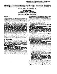
Fig. 1. Representation in form of hierarchical structure of a taxonomic arrangement of the items

Let G be a taxonomy represented in form of hierarchical structure over the items in I (see Figure 1) and organised by subtype-supertype (or is-a) relationships. The items at lowest levels are named as leaf items, those at intermediate levels as inner items, while the items at highest level as root item. An edge xi ← yj in G denotes a subtype relationship: the item xi is the direct subtype of yj , or conversely, the item yj is the direct supertype of xi . An item z is a supertype of xi if there is a path from xi to z (xi is a subtype of z). A transaction T supports an item yj ∈ I when yj ∈ T or ∃ xi ∈ T such that yj is a supertype of xi . An itemset Y is called multiple level itemset if it does not contain an item and its supertypes as well. An itemset Y is a supertype itemset of an itemset X, if Y can be obtained by replacing one or more items in X with one of their supertypes and |X| = |Y| (conversely X is a subtype itemset of Y). Given an itemset Y and Z one of its subsets, Z⇒ Y-Z is called multiple level association rule if no one of the items contained in the antecedent Z (conversely, consequent Y-Z) is supertype of any item contained in the consequent Y-Z (conversely, antecedent Z). Interestingly, rules containing items from the upper taxonomic levels represent more generalized information, conversely, those containing items from the lower levels represent more specialized information. Now we introduce some preliminary notions for explaining our contribution: – dXi be a function which maps I into a set of positive integer numbers, where dXi (xi )=1 iff xi is the root item in G, otherwise dXi (xi )= dXi (direct supertype (xi )) +1; – dX be a function which maps I into a set of positive integer numbers, where dX (X)= max(dXi (xi )), xi in X. – h be the composition f˚g where f and g are defined as follows:

Mining Multiple Level Non-redundant Association Rules

255

• f(D’): ℘(D’)→ ℘(I’), which associates with D’ the items common to all the transactions tk ∈ R and returns the set { xi ∈ I’ | ∀ tk ∈ D’, (tk , xi ) ∈ R }; • g(I’): ℘(I’) → ℘ (D’), which associates with I’ the transactions related to all items xi ∈ I’ and returns the set { tk ∈ D’ | ∀ xi ∈ I’, (tk , xi ) ∈ R }; where R⊆ D×I is a binary relation with I’⊆ I, D’⊆ D. The function h is commonly called Galois closure operator [6],[13]. Now it is worth of reminding that: i. an itemset X ⊆ I is closed iff h(X)=X. Moreover from [13] it follows that X is closed if none of its supersets has the same support as X (i.e., s(h(X))=s(X)); ii. given an itemset X and xi ∈ I: g(X)⊆ g( xi  ) ⇔ xi ∈ h(X) [12]; The concept of closed itemset is fundamental in this work: we extend it to the case of taxonomically organized items for removing redundant multiple level itemsets. In formal terms we have: Definition 1 (Multiple Level Closed Itemset). Let Y be a multiple level itemset, Y= y1 , y2 ,. . . , yj ,. . . ,yh , it is called multiple level closed itemset(mCI) iff: 1. item w, w ∈ I, w ∈ / Y, w is not supertype of yj ∈Y; 2. dX (Y) ≥ dXi (w); 3. | g(Y) - g(w )| ≤ ,  positive user-defined threshold (when =0 g(Y) ⊆ g(w )). It can be argued in this way. Assume =0 (for the sake of simplicity) and suppose an item w which is neither contained in Y and nor supertype of yj (yj ∈Y), and Y y1 , y2 ,. . . , yh  a closed itemset where g(Y)⊆g(w). This means that an itemset Y’ so composed  y1 , y2 ,. . . , yh , w exists and meets the relationships g(Y’)=g( y1 , y2 ,. . . , yh , w)= g(Y) ∩ g(w). Since g(Y) ∩ g(w)=g(Y) it follows that s(Y’)= s(Y), and then, according to the relation s(h(Y))=s(Y), Y is not closed itemset: this is in contradiction with the initial hypothesis, and then validates the conditions in Definition 1. Moreover, by the third condition of Definition 1 we know that an itemset X is redundant w.r.t Y if Y is supported by at least the same number of transactions that supports X, and if X and Y are supported from common transactions (respect to the  threshold). An explanatory toy example follows. Example 1. Consider the taxonomy in Figure 2, the transaction set in Table 1,  as 0 and the item w=B. It can be derived that the itemset A is a mCI while the itemset A11 ,A12  does not. Indeed, since g(A) is {1,2,3,4,5,6} and g(B) is {1,2,3,5} the relationship g(A)⊆ g(B) does not hold, hence B ∈ / h(A), finally A is a mCI (point ii presented above). On the contrary, g(A11 ,A12 )={3,5}, hence the relationship g(A11 ,A12 )⊆ g(B) does hold, then B ∈ / h(A11 ,A12 ), finally A11 ,A12  is not a mCI. Trivially it holds for any subtype of B.

256

C. Loglisci and D. Malerba

Table 1. A toy set of boolean transaction on leaf items. The taxonomic arrangement is reported in Figure 2. Transaction 1 2 3 4 5 6

A11 1 0 1 1 1 0

A12 0 1 1 0 1 0

B11 1 0 1 0 1 0

B12 1 0 1 0 1 0

A1 1 1 1 1 1 0

A2 1 0 0 1 1 1

B1 1 0 1 0 1 0

B2 1 1 1 0 1 0

A 1 1 1 1 1 1

B 1 1 1 0 1 0

Fig. 2. Representation of the taxonomy over the items for the example in Table 1

Considering the formal framework thus far described, the problem of interest in this work can be formulated as follows: Given: D transaction set, I set of items, G a taxonomy over the set I, minsup, minconf user-defined minimal thresholds for support and confidence, and  as user-defined value. Goal: 1. Finding out the set of multiple level closed frequent itemsets (mCFI) w.r.t. to  such that the support of each mCFI exceeds minsup; 2. Generating the set of multiple level association rules (mAR) exceeding the value of minconf. In the following two sections we present the computational solutions to these sub-problems.

4

An Algorithm for Finding Out the Multiple Level Closed Frequent Itemsets

The first sub-problem is here solved with an algorithm, named DELIS (DEscending Levels and Increasing Size) which scans the taxonomy in top-down way while, at each level, generates mCFIs with increasing size (or length). In particular the scanning strategy is based on a suitable order relation ”≺” over the items, which meets the following:

Mining Multiple Level Non-redundant Association Rules

given a set of items

1

257

I, a taxonomy G over I, a function O: I→ {1,2,. . . ,|I|},

i. xi ≺ xj (∀ xi ,xj ∈ I) iff dXi (xi ) = dXi (xj ) and O(xi )< O(xj ) (e.g., in Figure 2 O(A1 )=2, O(A2 )=6: A1 ≺ A2 ); ii. xi ≺ xik ≺ xj (∀ xi ,xj ∈ I, ∀ xik direct subtype of xi ) iff dXi (xi )= dXi (xj ), dXi (xik )= dXi (xi )+1 and O(xi ) < O(xik )< O(xj ) (e.g., in Figure 2 O(A1 )=2, O(A2 )=6, O(A11 )=3: A1 ≺ A11 ≺ A2 ); m iii. given two itemsets X1 , X2 , |X1 | = |X2 | = n, dX (X1 )≤ dX (X2 ), ∃ xm i xj , m m m≤n, the m-th items of X1 , X2 respectively, xi ≺ xj : X1 ≺ X2 . As we will see in the description of the algorithm 1 such a order relation permits: – to return frequent itemsets only if their supertypes are frequent too; – to generate frequent k-itemsets by joining frequent (k-1)-itemsets; – to consider closed frequent itemsets only if their supertypes are closed frequent too. At this aim the algorithm exploits the theorem reported below. Theorem 1. Let X1 =  x1 , x2 ,. . . , xj ,. . . ,xh  be an itemset, X’1 =  x1 , x2 ,. . . , x’j ,. . . ,xh  its subtype itemset, xj supertype of x’j , X1 is not a closed itemset: X’1 is not a closed itemset. Proof : Assume  as 0 and X1 is not a closed itemset. By resorting to the point ii in the previous section it is possible considering that it exists an item of I xk ∈ / X1 such that the relationship g(X1 ) ⊆ g(xk ) holds and xk ∈ h(X1 ). Hence it follows that g(X’1 ) ⊆ g(X1 ) ⊆ g(xk  ), namely g(X’1 ) ⊆ g(xk ) holds, where xk ∈ h(X’1 ) and xk ∈ / X’1 : it results that X’1 is not a closed itemset.  Finally we report an high-level description of DELIS algorithm (see Algorithm 1), where – h represents the size of the current multiple level frequent itemsets; – k indicates the current level of the taxonomy; – mFIh,k represents a set containing the multiple level frequent itemsets with size h generated at the level k ; – mCFI represents a set containing the multiple level closed frequent itemsets; – lowerLevel(G,k) returns the lower level of the taxonomy G w.r.t. the level k ; – frequentItemsGeneration(k) returns frequent items at level k. It also exploits the set of frequent items in mFI1,k−1 if k=lowerLevel(G,); – join(Xi ,Xj ) joins a la apriori Xi ,Xj [1], where Xi ≺ Xj ; – frequentItemsetsGeneration(mFIh,k−1 ) returns the multiple level frequent itemsets with size h generated at the level k: ∀ Xi ∈ mF I h,k−1 ’ Xi =  join(X’i ,X”i ), |X’i |=|X”i |=h-1, dX (X’i )≤k-1 and dX (X”i )≤k-1, it joins Xdi      with X”i , Xdi with X’i and Xdi with Xdi where dX (Xdi )=k or dX (Xdi )=k,   Xdi subtype itemset of X’i , Xdi subtype itemset of X”i respectively; 1

Without generality loss, we assume that the set of transactions D contains only leaf-items of the taxonomy.

258

C. Loglisci and D. Malerba

– getClosed(mFIh,k ) returns the multiple level closed frequent itemsets from mFI by exploiting Definition 1 and Theorem 1; – getGenerator(mCFIh,k ) returns the generator frequent itemsets from mFIh,k . We provide the definition of generator in the next section, where it is also used for the rule generation; – CG indicates the total set of generators; – leafItemLevel represents the lowest level of the taxonomy. A trace of the algorithm 1 follows. Consider the toy example reported in Table 1, minsup=0.4 and for the sake of simplicity =0. First (step 4), given h=1 and k=taxonomy level 1, mFIh,k = {A,B} is determined. Then (steps 5-12), at the current level of taxonomy, the frequent itemsets with larger length are determined (i.e., mFIh,k ={A,B}), moreover, by exploiting the Definition 1, the step 10 finds the closed ones (i.e., {A,A,B}) that will be also used at k=taxonomy level 2. From the step 13 the algorithm iteratively goes down the lower levels of taxonomy by scanning only the direct subtypes of closed frequent itemsets: at the step 15, given h=1 and k=taxonomy level 2, mFIh,k ={A1 , A2 }, B2 } where A2 , B2  are not closed because of A1 . Then, at the step 21 with h=2 mFIh,k consists of {A1 ,A2 ,A1 ,B2 }, A2 , B2 }, and at the step 23 the algorithm updates mFIh,k with {A,B2 ,A1 ,B,A2 ,B}. By exploiting Definition 1 at the step 24 only the frequent itemsets which are subtype of closed itemsets have to be proven as closed. Finally, given h=3 mFIh,k consists of {A1 ,A2 ,B2 ,A1 ,A2 ,B}.

5

Operative Definitions for Generating Multiple Level Minimal Association Rules

The algorithm DELIS generates the mCFIs which indeed constitute a subset of the complete set of mFIs: in [5] has been proven that mFIs can be inferred from mCFIs. Moreover, the rules generated with mCFIs (mAR) are indeed a minimal set of those discovered with mFIs, or, in other words, they are a non-redundant subset. In formal terms the notion of minimal rule [5] states that Definition 2 (Minimal Rule). An association rule R1 :A1 ⇒C1 is called minimal iff there does not exist R2 :A2 ⇒C2 with s(R1 )=s(R2 ), c(R1 )=c(R2 ), A2 ⊆ A1 , C1 ⊆ C2 . Now, our interest is to generate the rules from mCFIs and at this aim we provide a set of operative definitions. In literature it has also been proven that the mAR can be seen as the union of two sets, namely ExactRuleSet and ApproximateRuleSet respectively, which are computed by exploiting the following: Definition 3 (ExactRuleSet and ApproximateRuleSet). Let mCFI be the set of multiple level closed frequent itemsets and CG be the set of generators: the sets of rules ExactRuleSet and ApproximateRuleSet consist of rules with confidence respectively equals to 1 and smaller than 1. They correspond to the sets

Mining Multiple Level Non-redundant Association Rules

259

{Y⇒X-Y| X ∈ mCFI ∧ Y∈ CG ∧ Y generator of X ∧ s(X) = s(Y)} {Z⇒X-Z| X ∈ mCFI ∧ Z ∈ CG ∧ h(Z)⊆h(X)} A generator is defined as: Definition 4 (Generator Itemset). Let X be a closed itemset, and h the Galois closure operator: an itemset Y, |Y| >1, Y⊆I, is called generator of X (closed itemset) iff h(Y)=X and  Y’⊆I with Y’⊂ Y such that h(Y’)=X and s(Y’)=s(Y). Operatively ExactRuleSet is produced with rules of the form Y⇒X-Y where the relationships s(X)=s(Y) and h(X)=h(Y) hold, given c(Y⇒X-Y)= s(X∪Y)/ s(Y)=1, Y⊂ X and X as a mCI. Moreover, rules of the form Z ⇒X-Z can be derived from X and Y⇒X-Y considering that for each Z, where Y⊂ Z⊂ X, the relationship s(Z)=s(X)=s(Y) has to hold. Analogously, ApproximateRuleSet is composed of rules of the form Y⇒X-Y where the relationships s(X)