networks, over half of the events are in periodic patterns. Periodic patterns arise from many .... individual events and to sets of events. One approach to nding ...
Mining Partially Periodic Event Patterns With Unknown Periods� Sheng Ma and Joseph L. Hellerstein IBM T.J. Watson Research Center Hawthorne, NY 10532
Abstract Periodic behavior is common in real-world applications. However, in many cases, periodicities are partial in that they are present only intermittently. Herein, we study such intermittent patterns, which we refer to as p-patterns. Our formulation of p-patterns takes into account imprecise time information (e.g., due to unsynchronized clocks in distributed environments), noisy data (e.g., due to extraneous events), and shifts in phase and/or periods. We structure mining for p-patterns as two sub-tasks: (1) nding the periods of p-patterns and (2) mining temporal associations. For (2), a level-wise algorithm is used. For (1), we develop a novel approach based on a chi-squared test, and study its performance in the presence of noise. Further, we develop two algorithms for mining p-patterns based on the order in which the aforementioned sub-tasks are performed: the period- rst algorithm and the association- rst algorithm. Our results show that the association- rst algorithm has a higher tolerance to noise; the period- rst algorithm is more computationally e�cient and provides exibility as to the speci cation of support levels. In addition, we apply the period- rst algorithm to mining data collected from two production computer networks, a process that led to several actionable insights.
1 Introduction Periodic behavior is common in real-world applications [7][8][13] as evidenced by web logs, stock data, alarms of telecommunications, and event logs of computer networks. Indeed, in our studies of computer networks, over half of the events are in periodic patterns. Periodic patterns arise from many causes: daily behavior (e.g. arrival times at work), seasonal sales (e.g. increase sale of notebooks before a semester), and installation policies (e.g. rebooting print servers every morning). Some periodic patterns are complex. For example, in one network we discovered a pattern consisting of ve repetitions every 10 minutes of a port-down event followed by a port-up event, which in turn is followed by a random gap until the next repetitions of these events. 1
Our experience in analyzing events of computer networks is that periodic patterns often lead to actionable insights. There are two reasons for this. First, a periodic pattern indicates something persistent and predictable. Thus, there is value in identifying and characterizing the periodicity. Second, the period itself often provides a signature of the underlying phenomena, thereby facilitating diagnosis. In either case, patterns with a very low support are often of considerable interest. For example, we found a one-day periodic pattern due to a periodic port-scan. Although this pattern only happens three times in a three-day log, it provides a strong indication of a security intrusion. While periodic patterns have been studied, there are several characteristics of the patterns of interest to us that are not addressed in existing literature: 1. Periodic behavior is not necessarily persistent. For example, in complex networks, periodic monitoring is initiated when an exception occurs (e.g., CPU utilization exceeds a threshold) and stops once the exceptional situation is no longer present. 2. Time information may be imprecise due to lack of clock synchronization, rounding, and network delays. 3. Period lengths are not known in advance. Further, periods may span a wide range, from seconds to days. Thus, it is computationally infeasible to exhaustive consider all possible periods. 4. The number of occurrences of a periodic pattern typically depends on the period, and can vary drastically. For example, a pattern with a period of one day period has, at most, seven occurrences in a week, while one minute period may have as many as 1440 occurrences. Thus, support levels need to be adjusted by the period lengths. 5. Noise may disrupt periodicities. By noise, we mean that events may be missing from a periodic pattern and/or random events may be inserted. This work develops algorithms for mining partially periodic patterns, or p-patterns, that consider the above ve issues. We begin with establishing a looser de nition of periodicity to deal with items (1) and (2). Speci cally, we introduce an on-o� model consisting of an "on" segment followed by an "o�" segment. Periodic behavior is present only during the on segment. Our de nition of p-patterns generalizes the partial periodicity de ned in [7] by combining it with temporal associations (akin to episodes in [11]) and including a time tolerance to account for imperfections in the periodicities. Finding p-patterns requires taking into account items (3)-(5) above. We structure this as two subtasks: (a) nding period lengths and (b) nding temporal associations. A level-wise algorithm can be employed for (b). For (a), we develop an algorithm based on a chi-squared test. Further, we develop two algorithms for discovering p-patterns based on whether periods or associations are discovered rst. The performance trade-o�s between these two approaches are studied. We conclude that the association rst algorithm has higher tolerance to noise while the period- rst algorithm is more computationally 2
e�cient. We study e�ectiveness and e�ciency of the algorithms using synthetic data. In addition, we apply the period- rst algorithm to mining data collected from two production computer networks, a process that led to several actionable insights. Sequential mining[11][5][18][15][12] has been studied extensively, especially in domains such as event correlation in telecommunication networks [11], web log analysis[6][17], and transactions processing[7][15]. All these work focus on discovering frequent temporal associations[11][15][18]; that is, nding a set of events that co-occur within a prede ned time window. There has also been recent work in identifying periodic behaviors[7][8][13][16] closely related to our work. Ozden et. al.[13] study mining of cyclic association rules for full periodicities{patterns that are present at each cycle. As noted earlier, this is quite restrictive since periodicities may occur only intermittently. Han et. al.[7][8] study partially periodic patterns with the assumption that period lengths are known in advance or that it is reasonable to employ an exhaustive search to nd the periods. Yang et. al.[16] extend Han's work by introducing concepts from information theory to address noisy symbols. We note that these latter e�orts focus on symbol sequences, not time-based sequences. In addition, none of these studies study the e�ect of noise in the form of random occurrences of events of the same type as those in the periodic pattern. Nor do these studies address the problem of phase shifts or imperfections in the periodicity. This sequel is organized as follows. Section 2 formulates the problem addressed. Section 3 presents our algorithm for nding possible periods. Section 4 describes our algorithms for nding p-patterns with unknown periods. Section 5 discusses empirical assessments of our algorithms. Our conclusions are contained in Section 6.
2 De nitions and Problem Statement Fundamental to our work is the concept of an event. An event has two attributes: a type and an occurrence time.
De nition 1 Let A be a set of event types. An event is a pair (a; t), where a 2 A is an event type and t 2 R is the occurrence time of the event. An event sequence S is an ordered collection of events, i.e. f(a1; t1 ); (a2; t2); : : :; (aN ; tN )g, where ai 2 A is the event type of the i-th event. ti represents the occurrence time of the event, and tj � ti for 1 � j � i � N . Throughout, we use D to denote the set of events being mined.
An event type may have a complex structure. For example, we can encode host name and alarm type into event type and so a \port down" alarm sent from host X has a di�erent event type than a \port down" alarm sent from host Y. Often, it is desirable to consider just the times associated with a sequence of events.
De nition 2 A point sequence is an ordered collection of occurrence times. 3
G
G F E
F
D �
GG F E
E
GG F F E
D
D
D
�
�
��
G F
G E D
�� 7LPH
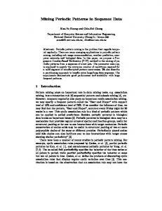
Figure 1: An illustrative event sequence. The event type of an event is labeled above its occurrence time.
2Q�VHJPHQW
3
�
2II�VHJPHQW
2Q�VHJPHQW 3�δS
�
�
��
�
�� 7LPH
1RLVH
Figure 2: The point sequence for event type \d" in Figure 1. \o" represents a \d" event. An event sequence can be viewed as a mixture of multiple point sequences of each event type. Figure 1 illustrates an event sequence, where the set of event types is A = fa; b; c; dg. The type of an event is labeled above its occurrence time. Figure 2 illustrates the point sequence of event type \d" Sd = (0; 3; 5; 6; 11; 12; 15; 19). A point is plotted as \o" at its occurrence time on the time axis. 0
Now, we de ne a periodic point sequence. We include the concept of tolerance to account for factors such as phase shifts and lack of clock synchronization.
De nition 3 S 0 = (t1; � � � ; tN ) is a periodic point sequence with period p and time tolerance � if a point occurs repeatedly every p � � time units. For example in Figure 1, the point sequence of event type \a" is Sa0 = (1; 5; 9; 13; 17). Thus, event type \a" is periodic with period 4. \b" is also periodic, if � � 1: The above de nition of periodicity requires periodic behavior throughout the entire sequence, which does not capture partial periodicities. To accomplish this, we consider a situation in which periodicities occur during on-segments and no periodicities are present during o�-segments. This is illustrated in Figure 2, where periodicities have a duration of p. 4
� time tolerance of period length Prede ned w a time window de ning temporal association Prede ned A1 a subset of event types A To be found by algorithms p period length To be found by algorithms minsup the minimum support for a p-pattern Prede ne; or computed based on p Table 1: Summary of parameters of p-patterns
De nition 4 A point sequence is partially periodic with period p and time tolerance �, if points are periodic with p and � during on-segments.
Referring to the above example, \d" and \c" are partially periodic with periods 3 and 2, respectively, but not periodic. Figure 2 illustrates the point sequence for \d", and its \on" and \o�" segments. Thus far, we have described periodicities of point sequences. This can be generalized to a set of events that occur close in time.
De nition 5 A set of event types A1 � A is a partially periodic temporal association (p-pattern)
with parameters p, � , w, and minsup, if the number of quali ed instances of A1 in D exceeds a support threshold minsup. A quali ed instance S1 � D satis es the following two conditions: (C1) The set of the event types of events in S1 = A1 , and where there is a t such that for all ei 2 S1; t � ti � t + w . (C2) The point sequences for each event type in S1 occur partially periodically with the parameters p and � .
To illustrate this de nition, we refer again to Figure 1. Let w = 1, � = 1, and minsup = 2. Then, fa; bg is a p-pattern with length 2 and period 4. Moreover, all non-null subsets of this pattern{ fag; fbg{are also p-patterns with length 2. It can be easily veri ed that p-patterns are downward closed. That is, if A1 is a p-pattern, then all non-null subsets of A1 are also p-patterns. This means that a level-wise search can be used, thereby providing computational e�ciencies.
2.1 Overview of Approach Table 1 summarizes the parameters of a p-pattern. w speci es the time window for temporal associations. p and � characterize a period length and its time tolerance. Herein, we assume that � , w, and minsup are given. Thus, nding p-patterns includes two sub-tasks: (1) nding (all) possible periods fpg, and (2) discovering temporal patterns A1 with w. We proceed as follows. Section 3 develops algorithms for nding possible periods. Section 4 develops 5
100
90
80
70
60
50
40
30
20
10
0
0
0.01
0.02
0.03
0.04
0.05
0.06
0.07
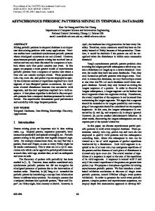
Figure 3: Distribution of inter-arrivals for a random point sequence. \-": empirical result. \..": theoretical distribution. \{": a threshold obtained by a chi-squared test. \-."': a constant threshold. algorithms to discover p-pattern with unknown periods by combining the two sub-tasks.
3 Finding Unknown Periods This section develops an e�ective and e�cient approach to nding periods in point sequences. E�ectiveness requires robustness to missing events and to random occurrence of additional events as well as dealing with partial periodicities. E�ciency demands that computations scale well as the number of events grows and the range of time-scales increases. Our approach to nding periods applies both to individual events and to sets of events. One approach to nding unknown periods is to use the fast Fourier transform (FFT), a well developed technique for identifying periodicities. There are two problems with doing so. First, the FFT does not cope well with random o�-segments in p-patterns. Further, the computational e�ciency of FFT is O(T log T ), where T is the number of time units. In our applications, T is large even though events are sparse. For example, although there may be several hundred thousands of events in a month at a medium-sized installation, there are over one billion milliseconds.
3.1 Chi-squared test for Finding Periods We begin with some notation. Let (t1 ; � � � ; tN ) be a point sequence in a time window [0; T ], where N is the total number of points. We denote the i-th inter-arrival time by �i = ti+1 ? ti ; where 1 � i � N ? 1: We de ne two extreme point sequences: an ideal partially periodic sequence and a random sequence. An ideal partially periodic sequence is modeled by a sequence of on-o� segments, in which a point re-occurs periodically during an \on" segment, and no point occurs during an \o�" segment (e.g., event "a" in Figure 1). A random point sequence is an ordered collection of random points generated randomly and 6
1
0.9
0.8
0.7
0.6
0.5
0.4
0.3
0.2
0.1
0
0
0.5
1
1.5
2
2.5
3
3.5
4
4.5
5
Figure 4: The e�ect of noise. y-axis: success percentage. x-axis: NSR ratio. "-": rst-order interarrival. "..": second-order inter-arrival uniformly in [0; T ]. Now, we characterize inter-arrivals for an ideal partial periodic point sequence with parameters p and �. Let �i = 1 if both ti and ti+1 are in the same on-segments; otherwise, �i = 0. When �i = 1, i.e. the i-th and (i + 1)-th arrivals are in the same on-segment, �i = p + ni , where ?� � ni � �; characterizes a random phase shift. When �i = 0, i.e. successive arrivals are not in the same on-segment, �i = ri , a random variable characterizing a o�-segment. Put these two cases together, we obtain �i = (�i)(p + ni) + (1 ? �i)r : (1) i
Now consider an arbitrary inter-arrival time � and a xed �: Let C� be the total number of arrivals with values in [� ? �; � + � ]. Intuitively, if � is not equal to p, C� should be small; otherwise Cp should be large. Based on this observation, an naive algorithm for nding periods is to look for large values of C� : That is, an inter-arrival � is declared to be a period, if
C� > thres:
(2)
However, there is a problem. Intuitively, the number of partially periodic points with a large p is much smaller than that with a small p given the same on-segment length. Therefore, the naive algorithm favors small periods. To illustrate this, we randomly and uniformly generate 1000 points in the interval [0; 100]. The solid line of Figure 3 plots the distribution of inter-arrivals. A threshold used by the naive algorithm is illustrated by the dash-dotted line. The gure shows that the distribution of inter-arrivals decays as inter-arrivals increase. As the naive algorithm employs a xed threshold regardless of period length, it tends to produce false positives for small periods and false negatives for large periods. Clearly, we need a threshold that adjusts with the period under consideration. One approach is to use a chi-squared test. The strategy here is to compare C� with the number of inter-arrivals in [� ? �; � + � ] 7
that would be expected from a random sequence of inter-arrivals. The chi-squared statistic [9] is de ned as C� ? NP� )2 ; �2� = (NP (3) � (1 ? P� ) where N is the total number of observations and P� is the probability of an inter-arrival falling in [� ? �; � + � ] for a random sequence. Thus, NP� and NP� (1 ? P� ) are the expected number of occurrences and its standard deviation, respectively. �2� is the normalized deviation from expectation. Intuitively, the chi-squared statistic measures the degree of independence by comparing the observed occurrence with the expected occurrence under the independence assumption. A high �2� value indicates that the number of inter-arrivals close to � cannot be explained by randomness, which is a necessary condition for periodicity.
�2 is usually de ned in terms of a con dence level. For example, 95% con dence level leads to �2 = 3:84. Then, the above equation can be changed to q
C�0 = 3:84NP� (1 ? P� ) + NP� :
(4)
C�0 can be used as a threshold to nd possible periods. That is, we say that � is a possible period, if C� > C�0 : (5) To compute P� , we note that a random event sequence approaches a Poisson arrival sequence[14] as the number of points increases. Further, it is well known that the inter-arrival times of a Poisson process are exponentially distributed. Using this, we obtain Z p+�
� exp(?�t)dt; P� = p?� � 2��exp(?�p);
(6) (7)
where � = N=T is the mean arrival. The approximation is obtained based on the assumption that �=p is small. We conducted simulation experiments to assess the accuracy of this result. Figure 3 plots the results. The x-axis is the period (expected inter-arrival times), and the y-axis is the count of inter-arrival times for a period. These curves depict: (i) the empirical density of C� for a simulated exponential interarrival distribution (solid line), (ii) the expected value of C� in the simulated data (dotted line), and (iii) Cp0 for 95% con dence level (dashed line). Observe that the �2 test results in a threshold that varies with period. Further observe that C� < C�0 in all cases, and hence there is no false positive.
3.2 Finding Periods in Noisy Data Here we consider the ability of our test to detect partial periodicities in the presence of noise. By noise, we mean the addition of randomly occurring events in either an on-segment or an o�-segment of the p-pattern. 8
This situation is best described with an example. Consider event \d" in Figure 2. This event has a period of 3 starting at time 0 and extending through time 18. However, there are also two noisy \d" events at times 5 and 11. Thus, the set of inter-arrival times are f3; 2; 1; 5; 1; 3; 3g: Clearly, noise events make it more di�cult to detect the underlying period. To gain more insight, we conducted a series of experiments. In each, there was a periodic point sequence with p = 2 in [0; 200]. We then gradually increase the number of noise points, which are generated uniformly and randomly. We quantify the noise by computing the ratio of the number of noise events to the number events in the partial periodicity. We refer to this as the noise-to-signal ratio (NSR). For each NSR, 1000 runs were conducted. A run is successful if the period is correctly identi ed (i.e. above 95% con dence level), and no false period is found. Figure 4 plots the results. The x-axis is NSR, and the y-axis is the fraction of successful runs. The solid line displays the results for this experiment. Note that the success rate is above 90% if NSR does not exceed 1. However, as NSR increases above 1, the success rate degrades rapidly. There is an intuitive explanation for the rapid drop-o� in success rate as NSR increases beyond 1. As suggested by the example above, the performance of our test degrades rapidly when noise points lie between periodic events. With more noise events, this becomes increasingly likely. We note, however, that a noise point in an o�-segment does less damage than one in an on-segment since the latter creates two inter-arrivals that do not have the period and deletes one that does. Thus, these experiments are in some sense a worst case since there is no o�-segment. Can we improve the performance of the above algorithm? Intuitively, we may increase the chance to detect the period if we take into consideration inter-arrivals between events separated by n other events. We refer to this as n-order inter-arrivals. Of course, this comes at a price|increased computational complexity. The dotted line in Figure 4 shows the performance of our test with second-order interarrivals. Note that the NSR value at which the success probability declines rapidly is close to 2, which is almost double the NSR value at which success probability declines rapidly when using rst-order inter-arrivals.
3.3 Implementation Details We now present an algorithm for nding periods based on the chi-squared test introduced earlier. Our discussion focuses on rst-order inter-arrivals. The algorithm for higher-order inter-arrivals is essentially the same. Let S be a point sequence. We assume that memory is larger than jS j as we need the maximum of jS j memory to hold counts in the worst case. This assumption is reasonable for a sequence of events of the same type since: (a) we only need to keep track of arrival instants and (b) this is a shorter sequence than raw data that contains a mixture of event types. When memory is problematic, indexing mechanism 9
such as CF-tree[19] can be used to control the total number of buckets. The algorithm takes as input the points si in S , the tolerance � , and con dence-level (e.g. 95%). 1. For i = 2 to jS j (a) � = si :time ? si?1 :time (b) If C� does not exist, then C� = 1 (c) Else, C� = C� + 1 2. AdjustCounts(fC� g; � ) /*Adjust counts to deal with time tolerance*/ 3. For each � for which a C� exists (a) Compute threshold C�0 based on Equation 5 (b) If C� > C�0 , then insert � into the set of periods being output Step (1) counts the occurrence of each inter-arrival time. Step (2) groups inter-arrival times to account for time tolerance � by merging into a single group counts whose � values are within within � of one another. Step (3) computes the test threshold. If the threshold is exceeded by the test statistic, a possible period is found, and inserted into results. This procedure is repeated until all event types are processed. It is easy to see that the above algorithm scales linearly with respect to the number of events. Further, the algorithm does not depend on the range of time scales of the periods.
4 Mining P-patterns With Unknown Periods As we discussed, mining p-patterns with unknown periods is combination of two tasks: (a) nding periods, and (b) nding temporal association. In this section, we rst overview algorithms for (b), i.e. mining associations. We then develop algorithms that combine the two tasks in di�erent ways: the period- rst algorithm and the association- rst algorithm.
4.1 Level-wise Algorithm, and Its Variation for Mining P-patterns with Known Period Many algorithms have been developed to e�ciently mine associations[3][1][4], most of which are variations of the Apriori algorithm[3]1. Here, we summarize this algorithm and its variation for mining temporal associations ([11]). Then, we show how such an algorithm can be applied to mining p-patterns with known periods. This is done in a way that extends the algorithms in [8][7] so as to consider time tolerance and temporal data (rather than just sequence data). In next section, we show how to mine p-patterns with unknown periods. All algorithmsthat can nd associationscan be used for (b) in theory. Here, we focus on the level-wise algorithm for demonstration purpose. 1
10
We begin with level-wise search. Let Lk and Ck be, respectively, the set of quali ed patterns and candidate patterns at level k. Given events D and C1 = fc 2 2A jjcj = 1g, where A is the set of event types and C1 is a set of patterns with length 1, the level-wise algorithm proceeds as follows. (1) (2) (3) (4) (5)
k =1; Count the occurrences in D for each pattern v 2 Ck Compute the quali ed candidate set: Lk = fv 2 Ck jv:count > minsupg Compute the new candidate set Ck+1 based on Lk if Ck+1 is not empty, k = k + 1 and goto (2)
Step (3) computes the quali ed candidate set Lk from Ck based on the supports. Step (4) computes a new candidate set Ck+1 based on the previous quali ed patterns in Lk . This is typically implemented by a join operation followed by pruning[2]. Step (2) counts occurrences of patterns in D. Step (3) and (4) are similar for nding di�erent patterns, while Step (2) varies based on the patterns to be found. In mining associations, Step (2) augments the count of a pattern (called an item set) v 2 Ck by 1, if v is a subset of a transaction (see [3] for details). This can be generalized to an event sequence by introducing a time window to segment the temporal sequence into \transactions". In particular, Step (2) in mining temporal associations augments the count of a temporal association v 2 Ck (also called an Episode by [11]), if v is a subset of event types in a time window [t ? w; t]2. Similarly, Step (2) in mining p-patterns with a known period augments the count of a p-pattern v 2 Ck , if v satis es two conditions: (a) v is a subset of event types in a time window [t ? w; t]; and (b) v is a subset of those in the pervious window [t ? p ? � 0 ? w; t ? p ? � 0], where 0 � � 0 � � is corresponding to a possible time shift. Note that (a) corresponds to Condition 1 of De nition 5 (qualifying an instance of a temporal association), and (b) addresses Condition 2 (qualifying an instance with partial periodicity).
4.2 Discovering P-patterns with Unknown Periods Now, we describe algorithms for mining p-patterns with unknown periods. Two steps are needed in achieving this goal: (1) nding the possible periodicities and (2) determining the temporal associations. These two steps can be combined in di�erent orders resulting in two di�erent algorithms: the period rst algorithm, and the association- rst algorithm. The former does step (1) and then step (2), while the latter does step (2) and then step (1). A hybrid algorithm is also possible.
4.3 Period- rst algorithm This algorithm operates by rst nding partial periodicities for each event type, and then constructing temporal associations for each period. 2
Please refer [11] for subtle details.
11
Let D be the set of events (sorted by time). The period- rst algorithm is described as follows: Period- rst algorithm
Step 1: Find all possible periods 1 Group D by event type 2 Find possible periods for each event type Step 2: Find patterns 3 For each period p 1. Find related event types Ap = fa 2 Aja has a period pg 2. C1 = fv 2 2Ap jjv j = 1g 3. Set support level sup(p), and window size w(p) 4. Find p-patterns with p Step 1 nds the possible periods for individual events using the algorithm described in the proceeding section. In particular, Line 1 groups events by type so that events in each group can be read out sequentially to nd possible periods using algorithm discussed in Section 3.3. Alternatively, this step can be implemented in parallel to nd periods for all event types simultaneously. However, tree indexing schemes, as those used in [19], are needed to handle a large number of events. Step 2 nds all patterns for each period. It rst nds event types Ap = fa 2 Aja has a period pg . It then seeds initial candidate set C1 and speci es the minimum support and window size. Last, the level-wise mining (Section 3.3) can be performed to nd p-patterns with known p. Further, we note that Step 2 can be done in parallel for each period to gain further reductions in data scans. The period- rst algorithm uses the periods discovered to reduce the set of event types considered for temporal mining and hence signi cantly reduce the computational complexity of Step 2. Our experience has been that jApj is much smaller than jAj. Another advantage of the period- rst algorithm is that the minimum support and the window size can be assigned separately for each period based on the period length and its support. This makes it possible to nd a pattern with a very low support because of a large p3 , while avoiding drastic increase of the search space. The computational complexity of Step 1 is determined by the group operation4 . For Step 2, complexity is the sum of the complexity of nding temporal associations for each Ap : There is, however, a disadvantage to this algorithm. If noise events are present, then our ability to In our experience, we let minimum support be minsup(p) = T=p�, and w(p) = p, where 0 � �; 1, the performance of this algorithm drops considerably. Even more extreme, at NSR in the range of 5 to 10, the period rst algorithm fails completely. Note that the CPU time drops for the period- rst as NSR increases. This is because the period- rst algorithm nds fewer periods and so there are fewer possible temporal 5
Our results are not sensitive to minsup. A typical minsup ranges from 0:1% � 1% of the total number of events.
15
120
100
CPU time (second)
80
60
40
20
0
0
100
200
300 size of events (1000)
400
500
600
Figure 5: Average run time vs. the number of events E�ectiveness Run Time(second) NSR Period- rst Association- rst Period- rst Association- rst 0:5 � 1 100% 100% 4.3 14.7 1�2 40% 100% 1.5 14.5 5 � 10 0% 100% 0.9 14.9 Table 2: Experimental results associations. In contrast, the association- rst algorithm still nds 100% of the p-patterns. One nal comment is of interest here. This relates to the nature of the low e�ectiveness of the period rst algorithm if NSR >> 1: Under such circumstances, the problem is false negatives as a result of the period detection algorithm. That is, we fail to identify p-patterns that are present rather than falsely identify p-patterns that are not present.
5.2 Production Data Now, we apply our algorithms to mine p-patterns in real data. Here, our evaluation criteria are more subjective than the last section in that we must rely on the operations sta� to detect whether we have false positives or false negatives. Two data sets are considered. The rst data set was collected from an Intranet containing hundreds of network elements (e.g., routers, hubs, and servers). The second data set was collected from an outsourcing center that supports multiple application servers across a large geographical region. Events in the second data set are mostly application-oriented (e.g. the cpu utilization of a server is above threshold), whereas those in the rst data set are both network-oriented events (e.g. a link is down for 16
a router) and application-oriented. An event in both data sets consists of three key attributes: host name, which is the source of the event; alarm type, which speci es what happened (e.g., a connection was lost, port up); and the time stamp of when the event occurred. In our preprocessing, we map each distinct pair of host and alarm type into a unique event type. The rst data set contains over 10,000 events with around 400 event types over a three-day period. The second data set contains over 100,000 events with around 3000 event types over a two-week period. Table 3 and Table 4 report our results for the two data sets by pattern size. Column 1 indexes the search level of the level-wise algorithm. Column 2 shows the size of Ck (i.e. the number of quali ed patterns at level k) at each level. Column 3 indicates the number of large p-patterns. Here, large p-patterns refer to p-patterns that are not a subset of other p-patterns. Three more columns are used to indicate the diversity of p-patterns found: column 4 shows the number of periods at each level; column 5 is the range (minimum to maximum) of the periods; and column 6 is the range (minimum to maximum) of the occurrence counts for the p-patterns at that level. As shown in the two tables, many p-patterns are present. Indeed, over 50% of the events are in partially periodic patterns. Thus, NSR < 1 and so the period- rst algorithm should be e�ective. Why are periodic behaviors so common here? Two factors contribute to this. The rst is a result of periodic monitoring that is initiated when a high severity event occurs (e.g., an interface-down event). The second factor is a consequence of installation policies, such as rebooting print servers every morning. Further insights can be drawn from our results. Note that the range of periods is quite large{from less than a second to one day. This has a couple of implications. First, FFT would be extremely ine�cient with such a range of time scales. A second implication is the importance of having algorithms that employ di�erent minimum supports. For example, the daily patterns have a support no more than 3 in the three-day data, and no more than 14 in two-week data. Thus, daily patterns can only be discovered if there is a small minimum support. We reviewed these patterns with the operations sta�. It turned out that many of the p-patterns related to underlying problems. The p-patterns with period 1-day and lengths 10 and 11 were found to relate to a periodic port-scan, a possible indicator of a security intrusion. The pattern with period 5-minutes and length 1 resulted from an incorrect con guration of a hub. The pattern with period 60 seconds and 1 was caused by a router that did not get the most current routing information. More details on the data and out results can be found in [10].
6 Conclusion This paper addresses the discovery of partially periodic temporal associations (p-patterns), a pattern that is common in many applications. An example of a p-pattern in a computer networks is ve 17
Level 1 2 3 4 5 6 7 8 9 10 11 12 13
Candi- p-patterns Min:Max Min:Max date size Periods count 100 28 0:1-day 6 : 680 307 22 0:300 3:689 938 5 0:30 3:8 1917 1 4 3 3010 5 4 3 3525 3 4 3 3104 0 2057 2 4:1-day 3 1017 0 366 1 1 day 5 91 2 1 day 5 14 1 20 20 1 1 10 21
Table 3: Experimental results of the rst data set
Level 1 2 3 4 5 6 7
Candi- p-patterns Min:Max Min:Max date size Periods count 1500 354 0:1-day 10:2258 804 340 0:1-day 10 : 1890 781 103 0:2700 12 : 132 378 63 4 : 1 ? day 14 : 160 148 24 30 1 ? day 14 : 51 39 16 300 21 : 51 4 4 300 18 : 54
Table 4: Experimental results of the Second data set
18
repetitions every 30 seconds of a port-down event followed by a port-up event, which in turn is followed by a random gap until the next ve repetitions of these events. Mining such patterns can provide great value. Unfortunately, existing work does not address key characteristics of these patterns, especially the presence of noise, phase shifts, the fact that periods may not be known in advance, and the need to have computationally e�cient schemes for nding large patterns with low support. We begin by de ning partially periodic patterns (p-patterns) in a way that includes on-o� segments, and phase shifts (via the tolerance parameter � ). Next, we construct an e�cient algorithm for nding the period of a partially periodic pattern using a chi-squared test, and we study the performance of the proposed algorithm in the presence of noise. Further, we develop two algorithms for discovering ppatterns based on whether periods or associations are discovered rst, and we study trade-o�s between these approaches. One result is that the association- rst algorithm has higher tolerance to noise while the period- rst algorithm is more computationally e�cient. In particular, using synthetic data we nd that the period- rst algorithm is three to ve times faster than the association- rst algorithm. On the other hand, the e�ectiveness (i.e., robustness to false negatives and false positives) of the period- rst algorithm degrades rapidly if the noise-to-signal ratio exceeds 1. Using these insights, we apply the period- rst algorithm to two types of event logs. Many p-patterns are discovered in the log, some of which led to diagnostic and corrective actions. One area of future work is to explore hybrid algorithms that provide a way to control the trade-o� between computational e�ciency and e�ectiveness. Our current work suggests a couple of possibilities in this regard. One is to use the association- rst approach but to limit the size of the temporal associations discovered before switching to the period rst algorithm. Another strategy is to focus on the algorithm for nding unknown periods. We observe that by considering n-order inter-arrivals (the time between events separated by n other events), we can increase robustness to noise. Thus, we could employ the period- rst algorithm but control the parameter n.
References [1] C. Aggarwal, C. Aggarwal, and V.V.V Parsad. Depth rst generation of long patterns. In Int'l Conf. on Knowledge Discovery and Data Mining, 2000. [2] R. Agrawal, T. Imielinski, and A. Swami. Mining association rules between sets of items in large databases. In Proc. of VLDB, pages 207{216, 1993. [3] R. Agrawal and R. Srikant. Fast algorithms for mining association rules. In Proc. of VLDB, 1994. [4] R.J. Bayardo. E�ciently mining long patterns from database. In SIGMOD, pages 85{93, 1998. [5] C. Bettini, X. Wang, and S. Jajodia. Mining temporal relationships with multiple granularities in time sequences. Data Engineering Bulletin, 21:32{38, 1998. 19
[6] R. COOLEY, J. SRIVASTAVA, and B. MOBASHER. Web mining: Information and pattern discovery on the world wide web. In Proceedings of the 9th IEEE International Conference on Tools with Arti cial Intelligence (ICTAI'97), 1997. [7] J. Han, G. Dong, and Y. Yin. E�cient mining of partially periodic patterns in time series database. In Int. Conf. Data Engineering, 1999. [8] J. Han, W. Gong, and Y. Yin. Mining segment-wise periodic patterns in time-related database. In Int'l Conf. on Knowledge Discovery and Data Mining, 1998. [9] H.O. Lancaster. The Chi-squared distibution. John Wiley & Sons, New York, 1969. [10] S. Ma and J.L. Hellerstein. Eventbrowser: A exible tool for scalable analysis of event data. In DSOM'99, 1999. [11] H. Mannila, H. Toivonen, and A. Verkamo. Discovery of frequent episodes in event sequences. Data Mining and Knowledge Discovery, 1(3), 1997. [12] T. Oates, M. Schmill, D. Jensen, and P. Cohen. A family of algorithms for nding temporal structure in data. In 6th Intl. Workshop on AI and Statistics, 1997. [13] B. Ozden, S. Ramaswamy, and A. Silberschatz. Cyclic association rules. In Int. Conf. Data Engineering, pages 412{421, 1998. [14] S.M. Roos. Introduction to probability and statistics for engineers and scientists. John Wiley & Sons, New York, 1987. [15] R. Srikant and R. Agrawal. Mining sequential patterns: Generalizations and performance improvements. In Proc. of the Fifth Int'l Conference on Extending Database Technology (EDBT). Avignon, France., 1996. [16] J. Yang, W. Wang, and P. Yu. Mining asynchronous periodic pattern in time series. In Int'l Conf. on Knowledge Discovery and Data Mining, 2000. [17] O. Zaane, M. Xin, and J. Han. Discovering web access patterns and trends by applying olap and data mining technology on web logs. In Proc. Advances in Digital Libraries ADL'98, pages 19{29, 1998. [18] M. Zaki. Fast mining of sequential patterns in very large databases, 1997. Technical Report URCS TR 668, University of Rochester. [19] T. Zhang, R. Ramakrishnan, and M. Livny. Birch: A new data clustering algorithm and its applications. Data Mining and Knowledge Discovery, pages 141{182, 1997.
20