dard tools for industrial inspection requires that such systems have extremely ... Image-based non-destructive testing or automated defect recognition (ADR) methods ... Produce second. Minkowski training model. Load first. Minkowski model,.
Image-Based Automated Defect Recognition via Statistical Learning of Minkowski Functionals Fei Zhao, Paulo R. S. Mendonça, and Robert Kaucic GE Global Research One Research Circle, Niskayuna, NY 12065, USA {zhaof,mendonca,kaucic} @research.ge.com
Abstract The adoption of image-based automated defect recognition (ADR) systems as standard tools for industrial inspection requires that such systems have extremely high levels of performance. To accomplish this goal it is often necessary to exploit every available constraint or information available about the specific inspection problem to be tackled. We propose an inspection method for the detection of flaws in aluminum castings that explores two broadly applicable assumptions: (i) defect-free industrial parts are abundant and standardized; (ii) statistically, the characteristics that distinguish defective from non-defective regions show no preferential a priori direction or orientation. The first observation leads to the use of a reference-based approach to ADR, in which a set of registered images of defect-free parts is used to build a statistical model for normalcy. The second observation suggests the use of Minkowski functionals, due to their invariance properties, to build signatures for the identification of defects. The proposed method was tested on 800 2D radiographic images of 100 aluminum cylinder heads. Our approach yielded a 100% detection rate with a 4% false alarm rate. These promising results demonstrate the potential of the approach.
1
Introduction
Image-based non-destructive testing or automated defect recognition (ADR) methods are common place in the manufacturing sector to control the quality of manufactured parts. One possible categorization of the different approaches followed by inspection systems is into reference- and non-reference-based methods. The last category refers to systems that do not explore template images of the object under inspection, often due
Load N defect free training images
Register all training images to one template image
Load testing image
Calculate second Minkowski functional on training data
Produce second Minkowski training model
Calculate first Minkowski functional on training data
Produce first Minkowski training model
Load second Minkowski model, produce second Minkowski response
Calculate second Minkowski functional on testing data
Load first Minkowski model, produce first Minkowski response
Register testing image to template image
Combine first and second Minkowski responses
Calculate first Minkowski functional on testing data
Figure 1: Block diagram of the reference-based ADR System using Minkowski functionals to find anomalies in cast aluminum parts. The ADR system consists of an offline training step on defect-free reference parts and an online testing step on production parts. Minkowski functionals are computed on neighborhood windows centered at each pixel throughout the image. The learning of the normalcy models and the detection of abnormalities/defects are described in the text.
to their unavailability. When such template or reference images can be used, referencebased methods, adopted in this work, are usually the best choice, since the use of reference images are a straightforward method to explore available prior knowledge about the particular inspection problem at hand. A variety of reference- and non-referencebased approaches for finding anomalies in industrial parts can be found in the literature. Good surveys of such techniques are given in [12, 10]. A key component of any ADR system is the feature or features used to make the good part/bad part decision. A feature is a distinctive signature that enables the distinction between interesting occurrences, such as defects, and normal variations in an object or image of interest. The use of many different features has been proposed in the ADR literature, including grey-level intensities [19], filter responses [9], Zernicke features [4], shape features [18], and co-occurance features [11], to name a few. An important requirement of such features is that they present relevant invariant properties, which in the context of this work means the ability to reflect certain changes displayed by the images due to the present of abnormalities but at the same time to be invariant to natural or allowed variation in the part under inspection. We will show that Minkowski functionals [16, 1] exhibit invariant properties that are particularly attractive to many ADR problems, justifying their adoption in the work here presented. A block diagram of the overall system is shown in Figure 1.
2
2
Minkowski Functionals
Minkowski functionals, including standard geometric parameters such as volume, surface area, and Euler number [13], are well known measures in the field of stochastic geometry. Since Minkowski functionals can be used to describe both the shape and morphology of sets, they are widely used in a number of files such as materials science, cosmology and medical image analysis [17][14][3]. Considering each pixel in the image as a complex and convex set, an object A in N-dimensional Euclidean space RN can be viewed as a union of compact and convex subset. In RN , there exist N + 1 Minkowski functionals Mn (A) with n = 1, 2, ..., N + 1 that describe the morphology of the body A. Computation of Minkowski functionals can be carried out through Hadwiger’s formula [1]: N!ωN Mn (A) = (N − n)!ωN−n
Z
φ (A ∪ gEn )µN (dg),
(1)
RN
where ω j is the volume of the unit ball in j dimensions. ω0 = 1, ω1 = 2, ω2 = π, ω3 = 4π/3. E j is any j-dimensional affine subspace of RN , φ (X) is the Euler characteristic of the set X, and µN is the Haar measure [2] in RN . Using a formula by Adler [17], equation (1) can be approximated by considering a simplicial complex [8] of hypercubes. Such hyper-cubes can be obtained by sampling L points of a hyper-cubic lattice of spacing a, applying the discrete Euler formula [16]: ωN 1 ωn ωN−n an L n n!(N − n + j)! × ∑ (−1) j fN−n+ j (A), N! j! j=0
Mn (A) =
where fi (A) is the number of elements of rank i (vertices, edges, faces, etc.) contained in A. For image analysis, the body A in RN is obtained from grey-scale image by thresholding. Given a grey-scale image I and threshold ρ, the excursion set I(ρ) is defined as the set of all pixels that have intensity greater than ρ. Considering each excursion set as a body in RN , the Minkowski fucntionals for image I are actually functions Mn (I(ρ)) of the threshold ρ. In our work, 2D radiograohic images are used for defect detection. Minkowski functionals in 2D, which represent perimeter, area and Euler number, are given by 1 f2 (I(ρ)), L π f1 (I(ρ)) M1 (I(ρ)) = ( − f2 (I(ρ))), 4aL 2 1 M2 (I(ρ)) = 2 ( f0 (I(ρ)) − f1 (I(ρ)) + f2 (I(ρ))), a L
M0 (I(ρ)) =
3
(2)
where f0 (I(ρ)) corresponds to the number of vertices in body I(ρ), f1 (I(ρ)) is the number of edges in I(ρ), and f2 (I(ρ)) is the number of squares in I(ρ), induced by imposing over I(ρ) an arbitrary square grid. A typical example of excursion sets is shown in Figure 2, and the corresponding Minkowski functionals, computed according to equation (2), are shown in Figure 3. Minkowski functionals have several nice properties that make them well suited to radiographic and other image-based detection problems. In particular, according to Hadwiger’stheorem [8], Minkowski functionals are “motion invariant”, that is, they are independent of a body’s position and orientation in space. In addition, they exhibit the additivity principle, that is, the Minkowski functional of the union of two bodies is the addition of the two bodies minus the functional of the intersection: Mn (B1 ∪ B2 ) = Mn (B1 ) + Mn (B2 ) − Mn (B1 ∩ B2 ) for any B1 , B2 ∈ RN . These properties are particularly useful in compensating for the variations in radiographic images.
3
Modeling of Minkowski Functionals
To learn the description of normality, W aligned defect-free training images with size X × Y are used to generate statistical models in a pixel by pixel fashion. Given pixel Ai = (xi , yi ) in training images, where xi ∈ {1, . . . , X},yi ∈ {1, . . . ,Y } and i ∈ {1, . . . ,W }, we extract a w × w neighborhood window NAi centered at Ai . Then we compute the first and second Minkowski functionals MnAi (NAi (ρ)) for pixel Ai in its neighborhood window NAi , where n ∈ {0, 1} and ρ is the intensity threshold. From our experiments, we observe that the third Minkowski functional (Euler number) doesn’t capture the normality very well. Therefore only first and second Minkowski functionals are used in our application. To represent Mikowski functionals discretely, intensity normalization is performed for training and testing images first, then a discrete set of threshold value ρ in {ρ j , j ∈ 1, . . . , K} with ρ j < ρ j+1 is produced. These threshold values are evenly distributed over the normalized intensity interval. Using this discrete set, Minkowski functionals MnAi (NAi (ρ)) can be normalized to same length K for all images, thus each Minkowski functional will be represented by a K-dimensional vector MAn i = (MnAi (NAi (ρ1 )), . . . , MnAi (NAi (ρK )). We assume that the Minkowski functionals at each pixel follow a joint Gaussian distribution,N (τnAi , ΣAn i ). This enables us to use W defect-free training images to learn maximum likelihood estimates of the mean Minkowski functionals, τnAi and the corresponding covariance matrix ΣAn i : τnAi =
1 W 4
W
∑ MAn i
i=1
Figure 2: Example of excursion sets. The image on the left shows one 2D XRay cylinder head image used in this application. The image on right shows the excursion sets obtained by thresholding the original image at threshold ρ. 5
Minkowski functional M0 versus threshold value 5 x 10
2
4
Minkowski functional M1 versus threshold value 4 x 10
Minkowski functional M2 versus threshold value 800 600
1.5
M2
M
1
400
M0
3 1
2
200 0.5
1 0 0
50
100 150 Gray−level value
200
250
0
0 0
50
100 150 Gray−level value
200
250
−200 0
50
100 150 Gray−level value
200
250
Figure 3: Example of computed Minkowski functionals. This figure depicts the Minkowski functionals M0 , M1 and M2 computed for the image in Figure 2.
and ΣAn i = (
1 W
W
∑ (MAn i − τnAi )(MAn i − τnAi )T).
(3)
i=1
Once the model is claculated, Mahalanobis distance is used as a distance measure between the pixel B = (x, y) in the testing image and it’s corresponding defect free training pixels Ai = (xi , yi ), i ∈ {1, . . . ,W }: q Dn (B) = (MBn − τnAi )T (ΣAn i )−1 (MBn − τnAi ). Pixels with Mahalanobis distances greater than a predefined threshold are labeled as potential defect pixels. Figure 5 shows one Minkowski functionals training and testing example on the same single pixel. As shown in Figure 5, the defect-free training data are tightly bounded in mean plus and minus three standard deviations region. This region defines the defect-free region. In Figure 5 (a) and (b), the Minkowski functionals curves for a defect-free testing pixel falls inside the defect-free region. In Figure 5 (c) and (d), 5
Figure 4: Boundaries of excursion sets. The boundaries in blue and red, for given values of ρ j−1 and ρ j+1 isolates the boundary in green, corresponding to ρ j such that ρ j−1 < ρ j < ρ j+1 .
the Minkowski functionals curves for a defect testing pixel falls outside the defect-free region. This pixel will be labeled as potential defect pixel. In general, the covariance matrix ΣAn i for the Minkowski functionals is full rank. Using a full rank covaraince matrix and a mean vector for each pixel is very memory intensive. For each model, it requires K(K +1)/2 parameters to describe the symmetric covariance matrix ΣAn i and K parameters to describe τnAi . Thus, we use a less memory-intensive model. Given three excursion sets NAi (ρ j−1 ), NAi (ρ j ), and NAi (ρ j+1 ) obtained at threshold ρ j−1 , ρ j and ρ j+1 , the boundaries of NAi (ρ j−1 ) and NAi (ρ j+1 ) isolate the boundary of NAi (ρ j ) from image region inside NAi (ρ j−1 ) and outside NAi (ρ j+1 ) as illustrated in Figure 4. This observation suggests that it may be possible to model the values of Minkowski functionals as random variables sampled from a Markov random field with a clique structure defined by values at pairs of neighbors corresponding to “adjacent” values for ρ [5]. These assumptions imply that the precision matrix SnAi = (ΣAn i )−1 will be a tridiagonal matrix [15]. Enforcing this tridiagonality constraint, the results in [6] show that the off-tridiagonal elements of ΣAn i can be recursively calculated from the tridiagonal values of ΣAn i as
ΣAni (i, i + 2) =
ΣAn i (i, i + 1)ΣAn i (i + 1, i + 2) ΣAn i (i + 1, i + 1)
for i = 1, . . . , M − 2 and ΣAni (i, j) =
ΣAn i (i, j − 1)ΣAn i ( j − 1, j) ΣAn i ( j − 1, j − 1)
6
for i = 1, . . . , M − 3 and j = i + 3, . . . , M. The tridiagonal values can be calculated directly using equation (3). With this simplification, we only need to save tridiagonal values for each ΣAn i . The number of parameters to describe ΣAn i (i, j) is reduced to 2K − 1. 145
90
Mean + 3Std Mean − 3Std Testing
140
Mean + 3Std Mean − 3Std Testing
80 70 60
Mink2
Intensity
135
130
125
50 40 30 20
120 10 115
0
5
10
15
20 25 Normalized Mink1
30
35
0
40
0
5
10
15
(a) 145
30
35
40
30
35
40
(b) 90
Mean + 3Std Mean − 3Std Testing
140
20 25 Normalized Intensity
Mean + 3Std Mean − 3Std Testing
80 70 60
Mink2
Intensity
135
130
125
50 40 30 20
120 10 115
0
5
10
15
20 25 Normalized Mink1
30
35
0
40
(c)
0
5
10
15
20 25 Normalized Intensity
(d)
Figure 5: Example of Minkowski functionals training and testing on the same single pixel. All Minkowski functionals are normalized to same length of 40. In each figure, the solid color curves show Minkowski functionals for defect-free training images. The dotted red curves represent mean plus and minus three standard deviations. The thick green curve represents the Minkowski functionals for testing image. (a),(b) show the first and second Minkowski functionals training and testing for a defect-free testing image. (c),(d) show the first and second Minkowski functionals training and testing for a defect testing image.
4
Implementation
A block diagram of the Minkowski functional-based ADR system in shown in Figure 1. A set of defect-free images, herein referred as the training set, are first registered to an arbitrarily selected image in the set. Then the Minkowski functionals for each pixel are calculated in its corresponding w × w neighborhood window. These pre-computed Minkowski functionals are used to build a statistical model of the probability distribution of the Minkowski functionals for each pixel as described in section 3 . Once the 7
model is computed, the Mahalanobis distance is used as the Minkowski response to decide whether or not the Minkowski functionals of a given new image are compatible with the probability distribution obtained from the training data. The training and testing for the first and second Minkowski functionals are performed separately. The last step is to obtain a combined response value by adding the Mahalanobis responses for the first and second Minkowski functionals. Pixels with responses greater than a threshold are identified as candidate defective pixels. Individual defect pixels are then grouped using connected components algorithm. The grouped clusters with size greater than a given size threshold are labeled as defects. The whole system was implemented in C++ using the Insight Segmentation and Registration Toolkit (ITK) [7].
5
Experiments
Minkowski functional-based features were used in a 2D radiograph inspection task to demonstrate their efficacy. Specifically, cast aluminum cylinder heads were inspected with a robotic system that positioned the cylinder heads at 8 different positions. One 2D radiographic image is taken at each position. Therefore, each single cylinder head part includes 8 2D XRay images corresponding to 8 view positions. Each 2D image has size 512 × 512. 200 defect-free parts are used for training. A 13x13 neighborhood window is used for Minkowski calculation at each pixel. 100 parts including 5 defect parts with total 6 individual defects and 95 defect free parts were used for testing. A correct identification is determined by correctly finding a defect in the appropriate view(s). A part is labeled as a false detection if a false indication is given in any of the 8 views. Our ADR system reached a 100% detection rate (6/6) with 4% false detection rate (4/100) as shown in table 1. Two example defect images with their corresponding Minkowski detections are shown in Figure 6. Actual/Detected Defect-free Defect
Defect-free 91 0
Defect 4 5
Table 1: Detection performance of ADR algorithm.
6
Conclusion
We have presented an ADR system that uses features computed from Minkowski functionals to identify defects in cast aluminum parts. Such features are a powerful new addition to the suite of features used in ADR systems. Minkowski functional features are motion invariant and exhibit the additivity principle. This makes them well suited for defect detection applications. 8
References [1] R. J. Adler and J. E. Taylor. Random Fields and Geometry. Birkhäuser, 2006. URL http://iew3.technion.ac.il/~radler/grf.pdf. 2, 3 [2] R. V. Ambartzumian. Factorization Calculus and Geometric Probability, volume 33 of Encyclopedia of Mathematics and Its Applications. Cambridge University Press, Cambridge, UK, 1990. 3 [3] V. AZavaletta, B. J. Bartholmai, and R. A. Robb. 3D morphological analysis of lung pathology. In ISBI, pages 308–311, 2007. 3 [4] H. Boerner and H. Strecker. Automated x-ray inspection of aluminum castings. IEEE Transactions Pattern Analysis and Machine Intelligence, 10(1):79–91, 1988. [5] S. Geeman and D. Geeman. Stochastic relaxation, Gibbs distribution and the Bayesian restoration of images. IEEE Trans. Pattern Analysis and Machine Intell., 6(6):721–741, Nov. 1984. 6 [6] Y. Huang and W. F. McColl. Analytical inversion of general tridiagonal matrices. J. Phys. A: Math. Gen., 3(22):7919–7933, 1997. 6 [7] L. Ibanez, W. Schroeder, L. Ng, and J. Cates. The ITK Software Guide. Kitware, Inc. ISBN 1-930934-15-7, http://www.itk.org/ItkSoftwareGuide.pdf, second edition, 2005. 8 [8] D. A. Klain. A short proof of Hadwiger’s characterization theorem. Mathematika, 42:329–339, 1995. 3, 4 [9] J. Kosanetzky and H. Putzbach. Modern x-ray inspection in the automotive industry. In Proceedings of the 14th World Conference on Non-Destructive Testing, 1996. [10] D. Mery. Automated radioscopic inspection of aluminum die castings. Materials Evaluation, 65(6):643–647, 2006. [11] D. Mery and M. Berti. Automatic dectection of welding defects using texture features. In International Symposium on Computet Tomography and Image Processing for Industrial Radiology, pages 281–289, 2003. [12] D. Mery, T. Jaeger, and D. Filbert. A review of methods for automated recognition of casting defects. Insight, 44(7):428–436, 2002. [13] J. R. Munkres. Topology. Prentice Hall, Upper Saddle River, NJ, USA, 2000. 3 9
[14] J. Ohser and F. Mucklich. Statistical Analysis of Microstructures in Materials ScienceIntegral. Wiley, 2000. 3 [15] H. Rue and L. Held. Gaussian Markov Random Fields. Number 104 in Monographs on Statistics and Applied Probability. Chapman & Hall/CRC, 2005. 6 [16] L. Santaló. Integral Geometry and Geometric Probability. Cambridge Mathematical Library. Cambridge University Press, 2nd edition, 2004. 2, 3 [17] J. Schmalzing and T. Buchert. Beyond genus statistics: A unifying approach to the morphology of the cosmic structure. The Astrophysical Journal, 482(1):L1– L4, June 1997. 3 [18] M. Sofia and D. Redouane. Shapes recognition system applied to the non destructive testing. In Proceedings of the 8th European Conference on Non-Destructive Testing, 2002. [19] A. Vincent, V. Rebuffel, V. Rebuffel, R. Guillemaud, L. Gerfault, and P. Coulon. Defect detection in industrial casting components using digital x-ray radiography. Insight, 44(10):623–627, 2004.
10
(a)
(b)
(c)
(d)
Figure 6: Images with defects and their Minkowski detections. (a) and (c): Defect images with the human labeled defect indication (red bounding box). (b) and (d): Minkowski functionals ADR detection results. The detection region is labeled with red overlay.
11