The OpenGL Shading Language is an example ... to the multiple OpenGL passes required to implement these ...... AHO A. V., JOHNSON S. C., ULLMAN J. D.:.
Graphics Hardware (2004) T. Akenine-Möller, M. McCool (Editors)
Mio: Fast Multipass Partitioning via Priority-Based Instruction Scheduling Andrew Riffel� , Aaron E. Lefohn�† , Kiril Vidimce† , Mark Leone† , and John D. Owens� � University
of California, Davis
† Pixar
Animation Studios
Abstract Real-time graphics hardware continues to offer improved resources for programmable vertex and fragment shaders. However, shader programmers continue to write shaders that require more resources than are available in the hardware. One way to virtualize the resources necessary to run complex shaders is to partition the shaders into multiple rendering passes. This problem, called the “Multi-Pass Partitioning Problem” (MPP), and a solution for the problem, Recursive Dominator Split (RDS), have been presented by Eric Chan et al. The O(n3 ) RDS algorithm and its heuristic-based O(n2 ) cousin, RDSh , are robust in that they can efficiently partition shaders for many architectures with varying resources. However, RDS’s high runtime cost and inability to handle multiple outputs per pass make it less desirable for real-time use on today’s latest graphics hardware. This paper redefines the MPP as a scheduling problem and uses scheduling algorithms that allow incremental resource estimation and pass computation in O(n log n) time. Our scheduling algorithm, Mio, is experimentally compared to RDS and shown to have better run-time scaling and produce comparable partitions for emerging hardware architectures. Categories and Subject Descriptors (according to ACM CCS): I.3.2 [Computer Graphics]: Graphics Systems; D.3.4 [Programming Languages]: Processors—Compilers
1. Introduction Recent advances in architecture and programming interfaces have added substantial programmability to the graphics pipeline. These new features allow graphics programmers to write user-specified programs that run on each vertex and each fragment that passes through the graphics pipeline. Based on these vertex programs and fragment programs, several groups have developed shading languages that are used to create real-time programmable shading systems that run on modern graphics hardware. The ideal interface for these shading languages is one that allows its users to write arbitrary programs for each vertex and each fragment. Unfortunately, the underlying graphics hardware has significant restrictions that make such a task difficult. For example, the fragment and vertex shaders in modern graphics processors have restrictions on the length of programs, on the number of constants and registers that may be accessed in such programs, and the control flow constructs that may be used. c The Eurographics Association 2004. �
Each new generation of graphics hardware has raised these limits. As an example, Microsoft’s DirectX graphics standard specifies the maximum size in instructions of vertex and fragment (pixel) shader programs, and graphics hardware has closely tracked these limits. For instance, the vertex shader 1.0 specification allowed 128 instructions, and the 2.0 and 3.0 specifications increased this limit to 256 and 512 instructions, respectively. Fragment programs have increased in instruction size even more quickly: while version 1.3 pixel shaders could only run 12 instructions, version 2.0 increased this limit to 96 instructions, and version 3.0 supports a minimum of 512 instructions (with looping allowing a dynamic instruction count of up to 65,536). This rapid increase in possible program sizes, coupled with parallel advances in the capability and flexibility of vertex and fragment instruction sets, has led to corresponding advances in the complexity and quality of programmable shaders. For many users, the limits specified by the latest standards already exceed their needs. However, at least two major classes of users require substantially more resources
To Appear at Siggraph/Eurographics Graphics Hardware 2004
for their applications of interest, and it is these users whom we target with this work. The first class of users we target are those who require shaders with more complexity than current hardware can support. Many shaders in use in the fields of photorealistic rendering or film production, for instance, exceed the capabilities of current graphics hardware by at least an order of magnitude. The popular RenderMan shading language [Ups90] is often used to specify these shaders, and RenderMan shaders of tens or even hundreds of thousands of instructions are not uncommon. Implementing these complex RenderMan shaders is not possible in a single vertex or fragment program. The second class of users we target use graphics hardware to implement general-purpose (often scientific) programs. This “GPGPU” (general-purpose on graphics processing units) community targets the programmable features of the graphics hardware in their applications, using the inherent parallelism of the graphics processor to achieve superior performance to microprocessor-based solutions. Like complex RenderMan shaders, GPGPU programs often have substantially larger programs than can be implemented in a single vertex or fragment program. They also may have more complex outputs; instead of a single color, they may need to output a compound data type. To implement larger shaders than the hardware allows, programmers have turned to multipass methods in which the shader is divided into multiple smaller shaders, each of which respects the hardware’s resource constraints. These smaller shaders are then mapped to multiple passes through the graphics pipeline; each pass produces results that are saved for use in future passes. The key step in this process is the efficient partitioning of the shader into several smaller shaders. Chan et al. call this the “multipass partitioning problem”. In their 2002 paper, they propose a solution to this problem with a polynomial-time algorithm entitled “Recursive Dominator Split” (RDS) [CNS∗ 02]. Currently, RDS is the state of the art in solving the multipass partitioning problem. ATI’s prototype Ashli compiler [BP03], for example, uses RDS to partition its input RenderMan and GL Shading Language shader programs into multiple passes for use on graphics hardware. The OpenGL Shading Language is an example of a language that requires solutions to the multipass partitioning problem such as RDS: it calls for shading language implementations to “virtualiz[e] resources that are not easy to count”, including the “number of machine instructions in the final executable” [KBR03]. Despite its success, RDS has two major deficiencies that have made it less than ideal for use in modern graphics systems. • First, shader compilation in modern graphics systems is performed dynamically at the time the shader is run. Con-
sequently, graphics vendors require algorithms that run as quickly as possible. Given n instructions, the runtime of RDS scales as O(n3 ). Even the heuristic version of RDS, RDSh , scales as O(n2 ). This high runtime cost makes RDS and RDSh undesirable for implementation in runtime compilers. • Second, RDS assumes a hardware target that can output at most one value per shader per pass. While the hardware targeted by RDS at the time conformed to this restriction, more modern hardware allows multiple outputs per pass, and the RDS algorithm does not handle this capability. Because allowing more outputs in each pass implies more operations that generate those outputs, supporting multiple render targets per pass increases the effective number of operations that can be scheduled in a single pass. In this work we present Mio, an instruction scheduling approach to the multipass partitioning problem that addresses these two deficiencies. Our algorithms have better complexity than RDS (O(n log n) in the average case and Ω(n2 ) in the worst case) and efficiently utilize multiple outputs per pass. In addition, though we do not explore this point in this work, our solutions will continue to be applicable as shader programs use control flow. The remainder of this paper is organized as follows. In the next section we describe the previous work in this field, and in Section 3 the RDS algorithm in detail. In Section 4, we describe our algorithms and techniques that we have developed to solve the multipass partitioning problem. We explain our experimental setup in Section 5 and our results and discussion in Section 6. Our future work is enumerated in Section 7 and we conclude in Section 8. 2. Previous Work Shading languages were introduced by Rob Cook in his seminal paper on shade trees [Coo84], which generalized the wide variety of shading and texturing models at the time into an abstract model. He provided a set of basic operations which could be combined into shaders of arbitrary complexity. His work was the basis of today’s shading languages, including Hanrahan and Lawson’s 1990 paper [HL90], which in turn contributed ideas to the widely-used RenderMan shading language [Ups90]. While these shading languages were not meant for interactive use, several recent languages target real-time shading applications. Olano and Lastra developed a shading language for the PixelFlow graphics system in 1998; three years later, Proudfoot et al. targeted the programmable stages of NVIDIA and ATI hardware with their Real-Time Shading Language (RTSL) [PMTH01]. Many of RTSL’s ideas were incorporated into NVIDIA’s Cg shading language [MGAK03], also aimed at modern graphics hardware. Other notable shading languages for today’s graphics processors include SMASH [McC01] and the OpenGL Shading Language [KBR03].
To Appear at Siggraph/Eurographics Graphics Hardware 2004
Peercy et al. implemented a shading compiler on top of OpenGL hardware [POAU00]; they characterized OpenGL as a general SIMD computer and mapped RenderMan shaders to this SIMD framework. To map complex shaders to the multiple OpenGL passes required to implement these shaders, they used compile-time dynamic tree-matching techniques. SGI offers a product based on this technology (featuring both compile-time and runtime compiler phases) called OpenGL Shader [SGI04]. 3. Recursive Dominator Split (RDS) The work of Chan et al. presented runtime techniques to map complex fragment shaders to multiple passes of modern programmable graphics hardware [CNS∗ 02]. Their Recursive Dominator Split (RDS) algorithm generates a solution to the multipass partitioning problem. RDS is successful at finding near-optimal partitions for a variety of shaders on a diversity of cost models. Their system, implemented on top of the Stanford Real-Time Programmable Shading System, used a cost function incorporating the number of passes, the number of texture lookups, and the number of instructions, and then optimized the resulting multipass mapping to minimize this cost function. They described two particular algorithms: RDS, which uses search to make its save/recompute decisions, and RDSh , which uses a heuristic instead. They conclude that RDSh runs faster than RDS at the expense of partition quality; also, they find that optimal partitions generated through exhaustive search are only 0–15% better than those generated by RDS (which, in turn, are 10.5% better than those generated by RDSh ). We first describe the assumptions made by RDS that motivate its design, then describe the algorithm itself.
Outputs per Pass RDS assumes a single output per pass, and that output can only come from a single node (though the shader hardware targeted by RDS actually outputs a 4-component vector per pass, RDS would not be able to combine a 3-component result from one operation with a 1-component result from a different operation in a single pass’s output). 3.2. The RDS Algorithm RDS begins by identifying multiply-referenced nodes in its input DAG and deciding whether the values generated at those nodes should be produced in a separate pass and saved or instead recomputed. It then starts at the leaves of the DAG and traverses the DAG in postorder, greedily merging nodes into as few passes as possible. Chan et al. present two algorithms to make the decision to save or recompute. The first, RDSh , uses a heuristic to make this decision: the value at the multiply-referenced node is recomputed only if the resource consumption in the recomputation uses less than half the maximum resources allowed (operations, registers, etc.) in a single pass. The second, RDS, combines RDSh ’s save-recompute heuristic with a limited search over evaluations of partitions created by both saving and recomputing multiply-referenced nodes. 3.2.1. Cost of RDS The runtime cost of both RDS and RDSh depends on the cost to check if a subregion can be mapped to a single pass; for n nodes in the input DAG, Chan et al. define this cost as g(n) and assume this cost is O(n). They then demonstrate that RDS scales as O(n2 ) · g(n) = O(n3 ) and that RDSh scales as O(n) · g(n) = O(n2 ).
3.1. Assumptions
3.2.2. Limitations in RDS
Minimization Criteria RDS’s primary goal in dividing a shader into multiple passes is to minimize the number of passes. This decision is motivated by the overhead incurred on each pass, which includes the cost of setting up and running the input through all stages of the graphics pipeline as well as the runtime and memory cost of texture storage of intermediate results. Consequently, Chan et al. indicate that “RDS was designed under the assumption that per-pass overhead dominates the overall cost.” Save vs. Recompute One core decision that RDS considers is how to handle multiply-referenced nodes in the shade tree. If a node is multiply referenced, RDS must make a decision whether to compute and save the value at that node for use by its multiple references, or instead whether to recompute the value of that node at each of its multiple references. Saving reduces the number of overall instructions; recomputing reduces the number of passes at the cost of an increase in the number of instructions. Structure of Shader Input RDS assumes its input shader is expressible as a directed acyclic graph (DAG).
The RDS algorithm has three major limitations. First, its runtime cost of O(n3 ) (or O(n2 ) for RDSh ) makes it undesirable for use in runtime compilers. Next, because RDS considers only a single connected region of its input DAG at any time, it cannot handle more than one output per pass (and is not easily extended to do so within its O(n3 ) runtime cost; in concurrent work, Foley et al. demonstrate a O(n4 ) algorithm that can spill multiple outputs per pass [FHH04]). Finally, because RDS assumes its input is structured as a single DAG, it cannot support flow control operations such as conditionals or loops. Recent hardware supports both multiple outputs per pass as well as control flow within a shader, so while these two limitations were not restrictions in 2002 hardware, they will be in the hardware of today and tomorrow. 4. Mio: An Instruction Scheduling Algorithm In this paper we present an alternate algorithm to solve the multipass partitioning problem. Our solution is motivated by
To Appear at Siggraph/Eurographics Graphics Hardware 2004
two goals. First, the limitations of RDS described above do not allow RDS-produced shaders to take advantage of important features of modern graphics hardware. Second, the runtime cost of RDS makes it unsuitable for use in the dynamic compilation environments used by the drivers of modern GPUs, as well as problematic for partitioning high-quality rendering or GPGPU shaders with thousands of instructions. To address these two deficiencies, we present our solution, called “Mio” (pronounced “mee-oh”). The name Mio is derived from the word “meiosis,” a process of cell division that produces child cells with half the number of chromosomes as their parents. In the same way, Mio divides large programs into smaller partitions. We begin by contrasting the assumptions made in the design of RDS (Section 3.1) to the assumptions we have made in the design of Mio. We next describe the technique of “list scheduling” that is the core of Mio’s scheduling algorithm, then describe Mio and its operation.
4.1. Assumptions Minimization Criteria Each recent generation of graphics hardware has allowed shader programs with greater resource limits than the previous generation. Specifically, the newest hardware can run more operations, access more textures, and use more constants and registers than the generation before. These increasing resource limits cause a shift in our minimization goal. While RDS attempts to minimize the number of passes in its solution, often at the expense of additional operations to recompute an intermediate result, Mio instead attempts to minimize the number of operations. RDS’s decision was valid given the characteristics of the hardware at the time: the hardware targeted by RDS, the ATI Radeon 8500, allowed only 16 operations on each pass. With a larger number of operations allowed per pass, however, the overhead per pass becomes less significant. As the number of operations allowed per pass continues to increase, optimizing shader runtime no longer requires minimizing the number of passes but instead becomes minimizing the number of operations. We show in Section 6.1 that the performance of shaders on modern graphics hardware is no longer limited by the number of passes but instead by the number of operations. Save vs. Recompute For a node with a value that is multiply-referenced, RDS decides whether to save or recompute that node’s value for each reference. Because we have chosen to optimize for the number of operations, we never recompute the value at a multiply-referenced node. Structure of Shader Input Like RDS, our current implementation of Mio requires that its input shaders be expressible as DAGs. List scheduling can potentially handle more complex input, however, which we briefly discuss in Section 7.
Outputs per Pass In contrast to RDS, Mio accounts for both scalar (1-component) and vector (4-component) datatypes and coalesces multiple operation results into a single output when appropriate. For instance, for graphics hardware with 4 4-vector outputs, Mio supports up to 16 scalar outputs. We make two explicit assumptions in determining the outputs per pass: 1. We prefer to fill all 4 entries in an output vector when possible. 2. We also prefer to use more available outputs per pass when possible. Together, these two assumptions imply that we use the maximum resources allowed by the hardware to communicate results between passes. Since the limited amount of these resources is often the limiting factor in creating efficient partitions, our assumptions allow us to create schedules with lower operation and pass counts than if we do not use all these resources. However, doing so may incur the cost of more memory bandwidth when compared to less aggressive inter-pass data communication. While this additional bandwidth cost may be a possible bottleneck, we note that the number of possible outputs per pass is growing much more slowly than the number of operations per pass, and thus the relative spill cost is decreasing with time. These assumptions also imply that the graphics hardware can use its memory bandwidth equally efficiently with scalar, 1-output-per-pass outputs and vector, n-outputsper-pass outputs. Though some hardware has a measured peak bandwidth that declines as the number of render targets increases, the newest NVIDIA hardware appears to maintain a constant bandwidth independent of the number of render targets [Buc04]. 4.2. List Scheduling With this work we redefine the MPP as a Precedence Constrained Job-Shop Scheduling Problem (PCJSSP), a wellknown problem in the compiler community. Among the problems analogous to the PCJSSP are instruction scheduling, temporal partitioning, and golf tee time assignment. The input to the PCJSSP is a list of jobs, the resources they require (including time), and the dependencies between them. The goal of the problem is to schedule each job to a shop (resource), respecting resource limitations while minimizing the overall time to complete all the jobs. The PCJSSP is a NP-complete problem, but the technique of list scheduling provides good and often near-optimal solutions to the PCJSSP in polynomial time. List scheduling is a greedy algorithm that tries to schedule jobs based on priority as those jobs become “ready.” A job is ready when all of its predecessors are scheduled and the results created by those predecessors are available. The list scheduling algorithm begins with the first time slot, scheduling jobs into that time slot based on job priority, until the
To Appear at Siggraph/Eurographics Graphics Hardware 2004
resources available during that time slot are exhausted or dependencies prevent the scheduling of any jobs. It then moves to the next time slot(s) and continues to schedule jobs until all jobs are scheduled. At all times it maintains a ready list of jobs. Initially this list consists of all jobs with no dependencies, but as jobs are scheduled, new jobs whose dependencies are now satisfied are added to the ready list. The effectiveness of list scheduling hinges upon how priorities are assigned to jobs. A bad priority scheme can cause the resulting schedule to be far from optimal. One popular and effective scheme is critical-path priority, which gives preference to jobs that have the most jobs (or time) between them and the final job or jobs. Another scheme with good performance is most-successors priority, which prefers to schedule jobs with the most dependencies as early as possible. Jain and Meeran provide a comprehensive review of jobshop scheduling techniques [JM98]. A representative example of an early analysis of list scheduling is from Landskov et al. [LDSM80]; Cooper et al. evaluate the conditions under which list scheduling performs well and poorly [CSS98]. Inagaki et al. have developed the state of the art in runtime list scheduling techniques that integrate register minimization into scheduling and feature efficient backtracking [IKN03]. We define the MPP as a job-shop problem in the following way. Jobs are defined as shader operations; resources include shader functional units, registers (varying, constant, texture, and output), and slots in shader instruction memory. The MPP differs from traditional instruction scheduling in two important ways. First, traditional job-shop instruction scheduling considers functional units as the primary resource and does not consider register allocation, whereas in the MPP we must consider not only functional units as resources but also many other resources (registers, outputs, textures, etc.). Second, to solve the MPP we must generate outputs that map to passes in graphics hardware. In the context of traditional instruction scheduling, we must produce a schedule that can be segmented into multiple passes; this requires that no more than k registers can be live at the breakpoint between passes, where k is the number of allowed outputs for each pass of the shader. These k results can then be saved into textures and used in future passes. 4.3. The Mio Algorithm Mio is an instruction-scheduling approach to the MPP. Mio’s goal is to schedule operations into the minimum amount of total time while respecting the limitations of the underlying hardware. Traditional list scheduling methods for modern superscalar microprocessors attempt to maximize the amount of instruction-level parallelism in their programs. To do so, they attempt to maximize the number of operations in their ready list, thus allowing a maximal opportunity for parallel instruction issue. This strategy motivates a “wide” traversal of their input DAGs, working on many subtrees at the same time. Modern microprocessors feature large reg-
1
2
3
5
4 6
1
2
4
3
5 6
7
7
(a) Traditional.
(b) Mio.
Figure 1: Traditional list scheduling priority schemes attempt to maximize the parallelism in their instruction stream. Mio, on the other hand, minimizes register usage. Here we consider a 7-operation DAG that must be partitioned into two passes. Note that the traditional method can issue all 4 operations in its first pass in parallel but must pass 4 temporaries between passes. Mio, on the other hand, chooses a different set of operation priorities to only require 1 temporary between its passes. ister files and register-renaming hardware to store the large number of temporary results that result from this traversal. Modern GPUs, on the other hand, have a severe limitation in their ability to store intermediate results across multiple passes. They are constrained by the number of rendering targets and the width of storage to each rendering target—ATI’s X800 and NVIDIA’s GeForce 6800, for instance, support fragment programs of hundreds of unique operations but can only store 4 4-vectors at the end of each pass. The “wide” traversal typical of today’s common list scheduling implementations is therefore poorly suited to graphics hardware because of the GPU’s limited ability to store intermediates. Instead, a list scheduling algorithm for GPUs must perform a “deep” traversal of its input DAG (Figure 1). The deep traversal attempts to wholly traverse a given subtree before another subtree is begun. This traversal produces an instruction schedule with less register usage at the cost of instruction parallelism. We now describe the Mio algorithm and its priority scheme. • We begin with two passes through the input to generate the traversal order T for the DAG. The first pass assigns a Sethi-Ullman number to each node of the DAG, which indicates the number of registers required to execute the subtree rooted at that node. For tree-structured inputs, Sethi and Ullman have demonstrated that scheduling higher-numbered nodes first minimizes overall register usage [SU70]. (The corresponding problem for DAGs is NP-complete; Aho gives heuristics for computing good DAG orderings [AJU77], but we have found simply using the Sethi-Ullman numbering on input DAGs gives acceptable results in our tests.) This pass is O(n) with the number of input nodes. • On our second pass, we visit each node using a postorder
To Appear at Siggraph/Eurographics Graphics Hardware 2004
depth-first traversal through the input DAG, preferentially choosing the node with the highest Sethi-Ullman number. We break ties in an arbitrary manner (in our implementation, we use a pointer comparison). This pass is also O(n) with the number of input nodes, and at its end, we have a traversal order T for all operations in the input DAG. After the two prepasses, we can now schedule operations. • We first insert all operations with no predecessors into the ready list. • Next, all operations in the ready list are considered for scheduling. The ready list is implemented as a priority queue and we choose the operation in the ready list with the highest priority. The priority is simple: nodes (representing operations) earlier in the traversal order T are preferred over nodes later in T . • We then attempt to schedule the highest priority node from the ready list. An incremental resource estimator determines if the node can be added to the current pass without violating hardware constraints (such as the number of temporary registers, textures, etc.). If the resource estimator rejects a node because of the number of operations or temporary registers (hard limits that affect all operations), we empty the ready list and end the pass. If that limitation is instead an input constraint that may vary depending on which operations are scheduled (textures, varyings, or uniforms), we remove the operation from the ready list but continue to attempt to schedule other operations with the hope that they will not violate the constraint. (One possible optimization that we do not implement is to increase the priority of operations that do not increase a critical resource when that resource is nearly exhausted.) We do allow the scheduling of an operation that temporarily overutilizes the number of outputs per pass with the hope that future operations will return the schedule to compliance. • After we successfully schedule an operation, we add its successor operations that no longer have any unscheduled predecessors to the ready list and begin scheduling the next highest priority operation. • If the ready list is empty, we have completed a pass. We then check if the number of outputs exceeds the hardware constraint. If so, we require a rollback to a point where the constraints of the hardware are met. To facilitate this rollback when necessary, after every operation is scheduled, we check to see if we violate the output constraint. If we do, we add the current operation to a rollback stack. We clear the stack if we later add a node that puts the scheduled pass back into compliance with the output constraint. If we reach the end of the pass and do not meet the constraints, we must unschedule each node on the stack to roll back to a schedule that does meet the constraints. One of the advantages of the list scheduling formulation is that any priority scheme can be used, not just the SethiUllman numbering we use here. More sophisticated and ac-
curate priorities could easily be integrated into the framework we have developed. 4.3.1. Analysis of Mio Runtime The major costs in using Mio to partition an input shader into multiple passes are the cost of the two prepasses, the cost of scheduling of each operation, the cost of the maintenance of the ready list, and the cost of rollback. Both prepasses are O(n) since each node must be visited only once. If we assume the cost of maintaining the ready list is r(n), with no rollback all operations can be scheduled in O(n) · r(n). Most implementations of a ready list take O(log n) time; we implement the ready list as a O(log n) priority queue (specifically a heap). Though Gabow and Tarjan have demonstrated that the overhead of a priority queue can be reduced to O(1) [GT83], the constants associated with their method are large enough that only extremely large shaders would run more efficiently than with O(log n) methods. Overall, then, with no rollback the expected runtime of Mio is O(n log n). Rollback adds an additional O(n) cost to the cost of scheduling all operations (assuming a rollback at each operation), making the worst-case overall cost Ω(n2 ). (Note that it is only necessary to calculate the priority queue once per node rather than once per visit to the node, so the cost is not Ω(n2 log n).) It is important to note, however, that we do not continue to schedule in the current pass after rolling back, so the number of rollbacks can never be more than the number of passes. As the number of outputs per pass increases, rollbacks become less frequent and the cost of rollback consequently decreases. Section 6.2 shows our results for compiler runtime. When resource constraints are violated, rollback is not the only option. We could instead change the priority scheme and attempt to repair the schedule, but this would likely impose a higher runtime cost in exchange for a potentially better schedule (and a greater algorithmic complexity). We could also consider priority schemes that analyze resource usage for subsets of the input DAG instead of only one operation at a time, but again, these schemes would impose additional runtime costs. 5. Experimental Setup We integrated Mio into ATI’s prototype Ashli compiler [BP03]. Ashli implements RDSh and all results in this paper are compared against Ashli’s RDSh implementation. To evaluate the effectiveness of Mio, we measured its performance on a variety of RenderMan shader programs. Both RDSh and Mio share the Ashli front end, which parses the shader into the DAG used by the RDSh and Mio back ends. We have attempted to select shaders that represent a variety of fragment program types, including ones with ample and
To Appear at Siggraph/Eurographics Graphics Hardware 2004
W OOD
M ATTE
P OTATO
10 4 1 67
2 4 0 9
13 6 1 148
Shader
BAT
U BER
M ONDO
Uniform Varying Textures Operations
7 0 0 352
36 4 3 88
128 4 41 559
Uniform Varying Textures Operations
Table 1: Shader Characteristics. Our shaders of interest are listed with their relevant resource demands and operation counts.
little texture usage and ones with many and few multiplyreferenced nodes. We use three surface shaders in our tests. The W OOD shader simulates wood grain; it is the same core shader used by Chan et al. [CNS∗ 02]. M ATTE is a simple matte surface shader. P OTATO is a more complicated surface shader that approximates a potato skin. We also use three lights. BAT outlines the silhouette of a bat within a spotlight. The U BERLIGHT (U BER) shader implements a complex lighting model representative of those used in computer-generated film production. The shader we use here is a simplification of Gritz’s implementation of Barzel’s lighting model [Bar97]. We augment U BER with 10 fake shadows, 15 shadow maps, and 25 slides to create M ONDO L IGHT (M ONDO), whose texture use is large enough to require multiple passes on even Pixel Shader 3.0 hardware. In each of our tests we combine one surface shader with N lights (designated as S URFACE L IGHT N). Relevant shader characteristics are summarized in Table 1. We report results on two hardware configurations, Mio48 and Mio64, that target ATI Radeon 9800 Pro limits. Mio48 allows 48 ALU and 32 texture operations per pass, while Mio64 allows 64 and 32. It is necessary to use these smaller limits for the results we present in the next section to create a more difficult partitioning problem due to smaller partitions, to allow runtime measurements on the ATI card, and to permit a comparison with Ashli’s implementation of RDSh , which does not yet handle larger shaders. Because of an inefficiency in the Ashli code generator (all results must be explicitly copied to output registers), Mio48 represents a lower bound for Mio performance (16 operations are reserved for copying results to pass outputs per pass, so only 48 operations are usable) and an upper bound, Mio64 (in which all 64 operations can be used for useful work). We expect that a more efficient code generator would put optimized results closer to Mio64. When compared to Mio48 and Mio64, all
1500 Rendering time (ms)
Shader
4R/4W 4R/3W
1000
4R/2W 4R/1W
500 0 10
100
1000
Operations/pass Figure 2: Runtime of a 5000-instruction shader for 4 reads/n writes (n = 1, 2, 3, and 4) as we vary the number of operations per pass.
RDSh results allow 64 ALU and 32 texture operations per pass. Compile-time and runtime results were generated on a 2.8 GHz Pentium IV system running Microsoft Windows XP with 1 GB of RAM. Compile-time measurements record only the partitioning part of the compiler. Runtime results were run on a pre-release NVIDIA GeForce 6800 (NV40) graphics card with 256 MB of memory and driver version 61.32 and a ATI Radeon 9800 Pro with 128 MB of RAM and the Catalyst 4.5 driver. All code is written in C++ and compiled using the Microsoft .NET 2003 compiler. 6. Results and Discussion To demonstrate the utility of Mio, we must answer four questions. First, we show that the assumptions we have made about the limitations of multipass performance are valid in Section 6.1. Next, in Section 6.2, we compare the compiler runtime of Mio to that of RDSh . We then analyze Mio’s generated code statically in Section 6.3 and the runtime of that code in Section 6.4. 6.1. Limitations of Multipass Performance Splitting a shader into multiple passes requires storing intermediate results at the end of each pass. These intermediate results can then be used in future passes. Because of the cost of each pass, RDS attempts to minimize the number of passes. In Section 4.1, we argue that the greater amount of resources available in modern GPUs motivates minimizing the number of operations instead. To test this hypothesis, we consider the relationship between shader size and shader runtime. We expect that shaders with a small operation count will be limited by pass overhead, while shaders with a large number of operations will instead be limited by the operations. We measure this relationship by constructing an artificial shader benchmark
To Appear at Siggraph/Eurographics Graphics Hardware 2004
Compile time (s)
2 RDSh Mio48
1
Mio64
0 0 4 2 6 8 10 Number of Uber Instances Figure 3: Compiler runtime of W OOD U BERN (N = 1–10) for RDSh and Mio. The upper and lower bounds for Mio (Mio64 and Mio48) are nearly identical. and varying the number of operations allowed per pass. Figure 2 shows this relationship. In this experiment, we render a 512×512 quad with a 5000-line fragment shader. The shader uses alternating DOT and ADD instructions and three total registers. On each pass we write to n 4-vectors of 32-bit floats (4 tests with n = 1, 2, 3, and 4). We switch between pbuffer surfaces between passes with no context switch and average the results over 20 consecutive tests. From this experiment we can see that for small numbers of operations per pass, the performance is highly dependent on the number of passes. This agrees with RDS’s assumption that minimizing the number of passes is paramount for the small operations per pass characteristic of the hardware targeted by RDS. However, as the number of operations per pass becomes larger, the pass overhead is no longer a factor. The breakpoint for this changeover appears to be roughly 100–200 operations, after which Mio’s assumption of minimizing operations rather than passes becomes more relevant.
Shader
ALU Ops
Tex Ops
Total Ops
Passes
W OOD U BER 1 RDSh Mio48 Mio64
231 243 219
12 18 15
243 261 234
7 5 4
W OOD U BER 10 RDSh Mio48 Mio64
1836 1870 1632
106 200 166
1942 2070 1798
48 48 40
M ATTE M ONDO 2 RDSh Mio48 Mio64
2853 2738 2347
197 395 368
3050 3133 2715
56 88 79
P OTATO BAT 5 RDSh Mio48 Mio64
1106 1146 996
55 144 130
1161 1290 1126
25 37 32
Table 2: Static results of generated code. generated operations allows us to draw conclusions about the quality of the code generated by each algorithm. The results for the W OOD U BERN, M ATTE M ONDO 2, and P OTATO BAT 5 shaders are shown in Table 2. Static Mio operation counts are comparable to RDSh operation counts, with Mio generally having more texture operations (due to more spills) and fewer arithmetic operations (due to no recomputation). Shaders compiled by Mio also generally have a comparable number of passes to RDSh . The most fragile part of our implementation is in the rollback decisions, and we believe rollback represents the largest potential area for improvement in these results. 6.4. Runtime Analysis of Generated Shaders
6.2. Compiler Runtime In Section 4.3.1 we asserted that the superior theoretical compile-time performance of Mio would result in faster compile times for shaders on Mio than on RDSh . Figure 3 shows the comparison for a set of W OOD shaders lit with N U BER lights for passes limited to 64 operations. We note that even the lower bound to Mio performance, Mio48, is superior to RDSh ’s runtime, and that RDSh ’s runtime grows more quickly as the problem size increases. For P OTATO BAT 5, the compile time for Mio48, Mio64, and RDSh , respectively, was 0.35, 0.34, and 0.79 seconds; for M ATTE M ONDO 2, 3.29, 3.22, and 3.58 seconds. 6.3. Static Analysis of Generated Shaders We next analyze the generated code from Mio and RDSh . Comparing the number of passes and the total number of
The ultimate test for a compiler is the execution time of its generated code. We use the internal frame counter of the Ashli viewer to measure frame rate results. Unfortunately, the Ashli viewer can only display shaders of a limited size, but we expect the static code results from Section 6.3 to be indicative of runtime performance. With small shaders with few partitions, we found equal performance between shaders partitioned with RDSh and with Mio48. For example, running M ATTE U BER 1 (4 passes using 3 intermediate texture storage buffers with RDSh , 3 passes using 4 buffers with Mio48), we measured 60 frames per second on the NVIDIA GeForce 6800 and 40 frames per second on the ATI Radeon 9800 Pro. However, the Mio48 partition’s greater use of intermediate texture storage, due to spilling to multiple render targets, caused a substantial hit in performance when its use of buffers was considerably greater than RDSh ’s partition. For example, adding a second
To Appear at Siggraph/Eurographics Graphics Hardware 2004
U BERLIGHT to M ATTE U BER 1 resulted in Mio’s partition using 6 passes and 10 buffers while RDSh ’s had 7 passes and 5 buffers. The RDSh partition ran more than twice as fast on the GeForce 6800 (30 frames per second against 12 for Mio48). We believe that runtime performance is correlated with the number of intermediate buffers but have not yet fully investigated why this is the case. We believe a significant reason for the slowdown we see with a large number of buffers is a buffer’s large memory footprint: a 512 × 512, 4-surface pbuffer takes 17 MB of texture memory, and for Mio partitions that use many buffers, we expect the lower performance is caused by texture memory thrashing. We note that allowing more operations per pass will reduce the relative cost of the spill and so we expect Mio’s runtime results will improve as we schedule to hardware with more resources; we describe other possible optimizations in the next section. 7. Future Work Mio marks only one point on what we hope will be a continuum of partitioning algorithms with tradeoffs between runtime and partition quality. On one hand, faster runtime algorithms (O(n)) are desirable for graphics systems that perform all compilation at runtime. On the other hand, more expensive algorithms that produce near-optimal partitions are equally useful in environments that permit a significant amount of compile-time work. We hope that the development of this family of algorithms will allow us to answer the question of whether it is better to continue to grow resource limits with each generation of graphics hardware or whether we should require the graphics system to virtualize the hardware and hide the need for multipass or other methods. We have begun to explore O(n) partitioning algorithms by removing the ready list and simply choosing the highest node in the Sethi-Ullman order; our initial results are promising, but a much more thorough analysis is required. For more complex algorithms, we will incorporate other information that is not currently used in generating our partitions. First, we need a more sophisticated cost function for spilling results at the end of a pass. Unlike RDS, Mio assumes all operations have the same cost, and that we should use all spill resources if possible, but we believe that judiciously reducing the amount of spilling at appropriate times will result in better runtime results. (For example, slightly increasing the number of passes and operations while significantly reducing the number of spilled results at the end of passes will almost certainly be an overall performance win.) We would also like to investigate alternate priority schemes within the list scheduling framework. How can we augment or replace Sethi-Ullman numbering to achieve better compile-time performance and code quality? Another interesting problem is the need to consider a higher level of scheduling: we should explicitly schedule passes in a multipass shader in order to maximize cache performance and
minimize the live memory footprint at any time. In addition, revisiting our recompute vs. save decision would be worthwhile: are there ever circumstances in practice for which recomputing would produce superior results? We are also interested in performing a more detailed study on the impact of multiple render targets. Informally we note a substantial increase in Mio’s partition quality and an equally substantial decrease in runtime as the number of render targets increases. (Simply allowing multiple render targets consequently makes the MPP a much simpler problem in practice.) For the small number of render targets we investigate here, this makes sense, but how does this trend continue as the number of render targets continues to increase? One noteworthy feature of list scheduling is its ability to handle inputs with flow control [BR91]. The newest shader instruction sets feature loops, branches, and procedure calls, all features that we do not consider in this work. We hope to adapt our list scheduling algorithm to efficiently handle shaders that use these control flow constructs. 8. Conclusion The major contributions of this work are the characterization of the multi-pass partitioning problem as an instruction scheduling framework and the development of a priority scheme for list scheduling that enables the generated schedules to best match the abilities of the graphics hardware. We show that Mio, the partitioning algorithm we develop in this paper, allows both better compile-time performance of the shader compiler as well as comparable partitions to the previous best method, RDS, all while supporting multiple rendering targets. The list scheduling techniques at the core of Mio will also be well-suited to more complex shaders in the future, shaders that require more resources from the graphics hardware and that use more complex control-flow structures. We hope this work spurs the development of highperformance, robust virtualizing shader compilers that will fully hide the multi-pass partitioning problem from shader developers and allow even the largest and most complex shaders to be efficiently mapped to graphics hardware. Acknowledgements Arcot Preetham and Mark Segal from ATI provided access to the Ashli codebase that we used as the substrate for our implementation. Arcot and Craig Kolb from NVIDIA both provided valuable technical assistance. We would also like to thank Brian Smits, Alex Mohr, Fabio Pellacini and the rendering research group at Pixar for their support and contributions to this work. Aaron Lefohn is supported by a National Science Foundation Graduate Fellowship. Funding for this project is through UC Davis startup funds and through a generous grant from ChevronTexaco.
To Appear at Siggraph/Eurographics Graphics Hardware 2004
References
[IKN03]
I NAGAKI T., KOMATSU H., NAKATANI T.: Integrated prepass scheduling for a Java just-intime compiler on the IA-64 architecture. In Proceedings of the International Symposium on Code Generation and Optimization (2003), pp. 159–168.
[AJU77]
A HO A. V., J OHNSON S. C., U LLMAN J. D.: Code generation for expressions with common subexpressions. Journal of the ACM 24, 1 (1977), 146–160.
[Bar97]
BARZEL R.: Lighting controls for computer cinematography. Journal of Graphics Tools 2, 1 (1997), 1–20. http://www.renderman. org/RMR/Shaders/BMRTShaders/ uberlight.sl.
[JM98]
JAIN A. S., M EERAN S.: A State-of-theArt Review of Job-Shop Scheduling Techniques. Tech. rep., Department of Applied Physics, Electronics and Mechanical Engineering, University of Dundee, Scotland, 1998.
[BP03]
B LEIWEISS A., P REETHAM A.: Ashli— Advanced shading language interface. ACM Siggraph Course Notes (2003). http://www.ati.com/developer/ SIGGRAPH03/AshliNotes.pdf.
[KBR03]
K ESSENICH J., BALDWIN D., ROST R.: The OpenGL Shading Language version 1.051. http://www.opengl.org/ documentation/oglsl.html, Feb. 2003.
[BR91]
B ERNSTEIN D., RODEH M.: Global instruction scheduling for superscalar machines. In Proceedings of the ACM SIGPLAN Conference on Programming Language Design and Implementation (1991), pp. 241–255.
[LDSM80] L ANDSKOV D., DAVIDSON S., S HRIVER B., M ALLETT P. W.: Local microcode compaction techniques. ACM Computing Surveys 12, 3 (1980), 261–294.
[Buc04]
B UCK I.: GPGPU: General-purpose computation on graphics hardware—GPU computation strategies & tricks. ACM Siggraph Course Notes (Aug. 2004).
[CNS∗ 02]
C HAN E., N G R., S EN P., P ROUDFOOT K., H ANRAHAN P.: Efficient partitioning of fragment shaders for multipass rendering on programmable graphics hardware. In Graphics Hardware 2002 (Sept. 2002), pp. 69–78.
[Coo84]
C OOK R. L.: Shade trees. In Computer Graphics (Proceedings of SIGGRAPH 84) (July 1984), vol. 18, pp. 223–231.
[CSS98]
C OOPER K. D., S CHIELKE P. J., S UBRAMA NIAN D.: An Experimental Evaluation of List Scheduling. Tech. Rep. 98-326, Department of Computer Science, Rice University, Sept. 1998.
[FHH04]
F OLEY T., H OUSTON M., H ANRAHAN P.: Efficient partitioning of fragment shaders for multiple-output hardware. In Graphics Hardware 2004 (Aug. 2004).
[GT83]
G ABOW H. N., TARJAN R. E.: A lineartime algorithm for a special case of disjoint set union. In Proceedings of the Fifteenth Annual ACM Symposium on Theory of Computing (1983), pp. 246–251.
[HL90]
H ANRAHAN P., L AWSON J.: A language for shading and lighting calculations. In Computer Graphics (Proceedings of SIGGRAPH 90) (Aug. 1990), vol. 24, pp. 289–298.
[McC01]
M C C OOL M.: SMASH: A Next-Generation API for Programmable Graphics Accelerators. Tech. Rep. CS-2000-14, Department of Computer Science, University of Waterloo, 20 April 2001. API Version 0.2.
[MGAK03] M ARK W. R., G LANVILLE R. S., A KELEY K., K ILGARD M. J.: Cg: A system for programming graphics hardware in a C-like language. ACM Transactions on Graphics (Proceedings of ACM SIGGRAPH 2003) 22, 3 (July 2003), 896–907. [PMTH01] P ROUDFOOT K., M ARK W. R., T ZVETKOV S., H ANRAHAN P.: A real-time procedural shading system for programmable graphics hardware. In Proceedings of ACM SIGGRAPH 2001 (Aug. 2001), Computer Graphics Proceedings, Annual Conference Series, pp. 159– 170. [POAU00] P EERCY M. S., O LANO M., A IREY J., U NGAR P. J.: Interactive multi-pass programmable shading. In Proceedings of ACM SIGGRAPH 2000 (July 2000), Computer Graphics Proceedings, Annual Conference Series, pp. 425–432. [SGI04]
SGI: OpenGL Shader, 2004. http://www. sgi.com/software/shader/.
[SU70]
S ETHI R., U LLMAN J. D.: The generation of optimal code for arithmetic expressions. Journal of the ACM 17, 4 (Oct. 1970), 715–728.
[Ups90]
U PSTILL S.: The Renderman Companion. Addison-Wesley, 1990.