Missing-feature approaches in speech recognition - IEEE Xplore

[Bhiksha Raj and Richard M. Stern]

[Improving recognition accuracy in noise by using partial spectrographic

]

information

Missing-Feature Approaches in Speech Recognition

D

© ARTVILLE & COMSTOCK

espite decades of focused research on the problem, the accuracy of automatic speech recognition (ASR) systems is still adversely affected by noise and other sources of acoustical variability. For example, there are presently dozens, if not hundreds, of algorithms that have been developed to cope with the effects of quasistationary additive noise and linear filtering of the channel [16], [23]. While these approaches are reasonably effective in the context of their intended purposes, they are generally ineffective in improving recognition accuracy in many more difficult environments. Some of these more challenging conditions, which are frequently encountered in some of the most important potential speech recognition applications today, include speech in the presence of transient and nonstationary disturbances (as in many factory, military, and telematic environments), speech in the presence of background music or background speech (as in the automatic transcription of broadcast program material as well as in many natural environments), and speech at very low signal-to-noise ratios (SNRs). Conventional environmental compensation provides only limited benefit for these problems even today. For example, Raj et al. [29] showed that while codeword-dependent cepstral normalization is highly effective in dramatically reducing the impact of additive broadband noise on speech recognition accuracy, it is relatively ineffective when speech is presented to the system in the presence of background music, for reasons that are believed to be a consequence of the nonstationary nature of the acoustical degradation.

1053-5888/05/$20.00©2005IEEE

IEEE SIGNAL PROCESSING MAGAZINE [101] SEPTEMBER 2005

This article describes and discusses alternative robust recognition approaches that have come to be known as missing feature approaches [9], [10], [20]. These approaches are based on the observation that speech signals have a high degree of redundancy—human listeners are able to comprehend speech that has undergone considerable spectral excisions. For example, normal conversation is possible with speech that has been either high- or low-pass filtered with a cutoff frequency of 1,800 Hz [17]. Briefly, in missing feature approaches, one attempts to determine which cells of a spectrogram-like time-frequency display of speech information are unreliable (or missing) because of degradation due to noise or to other types of interference. The cells that are determined to be unreliable or missing are either ignored in subsequent processing and statistical analysis (although they may provide ancillary information), or they are filled in by optimal estimation of their putative values. The application of missing feature techniques to robust automatic speech recognition has been strongly influenced by two complementary fields of signal analysis. Many of the mathematical approaches to missing feature recognition were first developed for the task of completing partially occluded objects in

frames, typically about 25 ms wide. From each frame, a power spectrum is estimated as 2 N−1 − j2π(n−mL)k/N Z p(m, k) = w(n − mL)x(n)e ,

(1)

n= 0

where Z p(m, k) represents the k th frequency band of the power spectrum of the m th frame of speech, w(n) represents a window function, x(n) represents the n th sample of the speech signal, L represents the shift in samples between adjacent frames, and N represents the number of samples within the segment. The power spectral components are often reduced to a smaller number of components using triangular weighting functions that represent the frequency responses of the filters in a filter bank that is designed to mimic the frequency sensitivity of the human ear X p(m, k) =

hk( j)Z p(m, j),

(2)

j

Mel Filter Index

where hk( j) represents the frequency response of the 20 k th filter in the filter bank. 18 The most commonly used 16 filter banks are the Mel fil14 12 ter bank [13] and the ERB 10 filter bank [21]. 8 6 Alternately, X p(m, k) may 4 be obtained by sampling 2 the envelope of signals at Time (s) Time (s) Time (s) the output of a filter bank (a) (b) (c) [25]. We will refer to both the power spectra given by [FIG1] (a) The “mel’’ spectrogram for an utterance of clean speech. (b) The mel spectrogram for the same (1) and the combined utterance when it has been corrupted by white noise to an SNR of 10 dB. (c) Spectrographic mask for the noise-corrupted utterance using an SNR threshold of 0 dB. power spectra of (2) generically as power spectra. visual pattern recognition [1]. In addition, there is a strong The power spectral components are compressed by a nonlininterchange of techniques and applications between missing feaear function to obtain the final time-frequency representation, X(m, k) = f(X p(m, k)), where f(·) is usually a logarithm or a ture recognition and the field of computational auditory scene analysis (CASA), which seeks to segregate, identify, and recogcube root. We assume, without loss of generality, that f(·) is a nize the separate components of a complex sound field [8]. The logarithm. The outcome of the analysis is a two-dimensional mathematics developed for missing feature recognition can be representation of the speech signal, which we will refer to as a applied to other types of signal restoration implicit in CASA, and spectrogram. Figure 1(a) shows a pictorial representation of the analysis approaches developed in CASA can be useful for the spectrogram for a clean speech signal. identifying degraded components of signals that can potentially When the speech signal is corrupted by uncorrelated additive be restored through the use of missing feature techniques. noise, the power spectrum of the resulting signal is the sum of the power spectra of the clean speech and the noise SPECTRAL MEASUREMENTS AND SPECTROGRAPHIC MASKS Yp(m, k) = X p(m, k) + Np(m, k), (3) Missing feature methods model the effect of noise on speech as the corruption of regions of time-frequency representations of the speech signal. A variety of time-frequency representations where Yp(m, k) and Np(m, k) represent the k th frequency may be used for the purpose. Most of them follow the same basic bands of the power spectrum of the noisy speech and the noise, procedure: the speech signal is first segmented into overlapping respectively, in the m th frame of the signal. Since all power


spectral terms are nonnegative, Yp(m, k) is nearly always greater than or equal to X p(m, k). (In reality, finite-sized samples of uncorrelated processes are rarely perfectly orthogonal, and the power spectra of two uncorrelated processes do not simply add within any particular analysis frame. To account for this, an additional factor of 2 X p(m, k)Np(m, k) cos(θ) must be included in (3), where θ is the angle between the k th term of the complex spectra of the speech and the noise. In practice, however, this term is usually small and can safely be ignored.) The SNR of Yp(m, k), the (m, k)th component of the spectrogram of the noisy signal, is given by X p(m, k)/Np(m, k). The SNR of the spectrogram varies with both time and frequency. Typically, for any level of noise, the spectrogram includes regions of very high SNR (which are dominated by contributions of the speech component), as well as regions of very low SNR (which represent the characteristics of the noise more than the underlying speech). The low SNR regions of the spectrogram adversely affect speech recognition accuracy. As the overall SNR of a noisy utterance decreases, the proportion of low SNR regions increases, resulting in worse recognition accuracy. In missing feature methods, it is assumed that all components of a spectrogram with SNR above some threshold T are reliable estimates of the corresponding components of clean speech. In other words, it is assumed that the observed value Y(m, k) of such components is equal to the value X(m, k) that would have been obtained had there been no noise. Spectral components Y(m, k) with SNRs below the threshold, however, are assumed to be unreliable and assumed not to represent X(m, k). They merely provide an upper bound on the true value of X(m, k), i.e., X(m, k) ≤ Y(m, k). The set of tags that identify reliable and unreliable components of the spectrogram are referred to as the spectrographic mask for the utterance. Recognition must now be performed with the resulting incomplete measurements of the speech signal, where only some of the spectral components are reliably known and the rest are essentially unknown. Figure 1(b) shows the spectrogram for the utterance in Figure 1(a) after it has been corrupted to 10 dB by white noise. Figure 1(c) shows the spectrographic mask for the utterance when a threshold of 0 dB is used to identify unreliable elements, with the black regions representing the values of m and k, for which the corresponding spectral values Z p(m, k) are to be considered reliable. While in practice there is no single optimal threshold [28], [33], Cooke et al. and Raj et al. have typically used thresholds that lie between 5 and −5 dB. Before we proceed, we must establish some of the notation and terminology used in the rest of the article. We represent the observed power spectrum for the m th frame of speech as a vector Yp(m) and the individual frequency components of Yp(m) as Yp(m, k). We assume that the final time-frequency representation consists of sequences of log-spectral vectors derived as the logarithm of the power spectrum. We represent the m th log spectral vector as Y(m) and the individual frequency components in it as Y(m, k). For noisy speech signals, the observed signal is assumed to be a combination of a clean

speech signal and noise. We represent the power spectrum of the clean speech in the m th frame of speech as the vector X p(m), the corresponding log-spectral vector as X(m), and the individual frequency components of the two as X p(m, k) and X(m, k), respectively. In addition, we represent the power spectrum of the corresponding noise and its frequency components as Np(m) and Np(m, k). We represent the sequence of all spectral vectors Y(m) for any utterance as Y and the sequence of all corresponding X(m) as X. For brevity, we refer to Y(m), X(m), and N(m) as spectral vectors (instead of log-spectral vectors) and to Y and X as spectrograms. We refer to the time and frequency indices (m, k) as a time-frequency location in the spectrogram and the corresponding components X(m, k) and Y(m, k) as the spectral components at that location. Ideally, recognition would be performed with X, the spectrogram for the clean speech (or with features derived from it). Unfortunately, the spectrogram X is obscured by the corrupting noise, resulting in the observation of a noisy spectrogram Y which differs from X. Every vector Y(m) in Y has a set of reliable components that are good approximations to the corresponding components of X(m). We represent the spectrographic mask that distinguishes reliable and unreliable components of a spectrogram by S. The elements of S may be either binary tags identifying spectral components as reliable or not with certainty, or they may be real numbers between zero and one that represent a measure of confidence in the reliability of the spectral components. For the rest of this section, we assume that the elements of S are binary. The spectrographic mask vector that identifies unreliable and reliable components of a single spectral vector Y(m) is represented as S(m). We arrange the reliable components of Y(m) into a vector Yr(m) and the corresponding components of X(m) into a vector X r(m). Each vector Y(m) also has a set of unreliable components that provide an upper bound on the value of the corresponding components of X(m). We arrange the unreliable components of Y(m) into a vector Yu(m), and the corresponding components of X(m) into X u(m). We refer to the set of all Yr(m) as Yr . Similarly, we refer to the set of all Yu(m), X r(m), and X u(m) as Yu , Xr , and Xu , respectively. The relationship between Yr(m), X r(m), Yu(m), and X u(m) is given by X r(m) = Yr(m) X u(m) ≤ Yu(m)

(4)

It is also common to assume a lower bound on X u(m), based on a priori knowledge of typical feature values. For instance, when the nonlinear compressive function f(·) used in the computation of the spectrogram is a cube root, X u(m) is assuredly lower bounded at zero. In some sections of the article, we drop the time and frequency-component indices of vectors, simply representing them as X, X r, and X u, where these vector indices are not critical to comprehension, for brevity of notation. This should not cause any confusion.


ADDITIONAL BACKGROUND In this section, we briefly describe three other topics that are of relevance to the rest of this article: speech recognition based on hidden Markov models (HMMs), bounded marginalization of Gaussian densities, and bounded maximum a posteriori estimation of Gaussian random variables. SPEECH RECOGNITION USING HMMS While the experimental results described in this article were obtained using HMMs, the concepts described are easily carried over to other types of recognition systems as well. The technology of HMMs has been described in detail in other sources [27], but we will summarize the basic computation briefly to introduce the notational conventions used in this article. Given a sequence of feature vectors X derived from an utterˆ the sequence of words in ance, ASR systems seek to identify W, that utterance per the optimal Bayesian classifier

ˆ = arg max{P(W|X)} = arg max{P(X|W)P(W)}. W W

W

(5)

P(W) is the a priori probability that the word sequence W was uttered and is usually specified by a language model. P(X|W) is the likelihood of X, given that W was the sequence of words uttered. The distribution of the feature vectors for W is modeled by an HMM that assumes that the process underlying the signal for W transitions through a sequence of states s from frame to frame. Each transition produces an observed vector that depends only on the current state. Let PW (X|s) denote the state output distribution of state s of the HMM for W. Ideally, P(X|W) must be computed considering every state sequence through the HMM. In practice, however, ASR systems attempt to estimate the best state sequence jointly with the best word sequence. In other words, recognition is performed as ˆ W = arg max max P(w)P(s|W) PW (X(m)|s) , W

s

(6)

m

where s represents the state sequence s1 , s2 , . . . , and P(s|W) is the probability of s as obtained from the transition probabilities of the HMM for W. The state output distribution terms PW (X|s) in (6) lie at the heart of how missing feature methods affect speech recognition. BOUNDED MARGINALIZATION OF GAUSSIAN DENSITIES Let a random vector X have a Gaussian density with mean µ and a diagonal covariance matrix . Let the indices of the components of X be segregated into two mutually exclusive sets, U and R. Let X u be a vector constructed from all components of X whose indices lie in U. Let X r be a vector constructed from all components of X whose indices lie in R. Let it be known that X u is bounded from above by Hu and below by Lu . It can be shown that the marginal probability density of X r is given by

−(X( j)−µ( j))2 1 e 2σ ( j) √ 2πσ ( j) j∈R H(l) −(x−µ(l))2 1 × e 2σ (l) dx, 2πσ (l) l∈U L(l)

P(X r, Lu ≤ X u ≤ Hu; µ, ) =

(7)

where the arguments after the semicolon on the left hand side of the equation represent the parameters of the distribution. X( j ), µ( j ), and σ ( j ) represent the j th components of X and µ and the jth diagonal component of , respectively. H(l ) and L(l ) represent the components of Hu and Lu that correspond to Y(l ). The integral term to the right marginalizes out X u within its known bounds. BOUNDED MAP ESTIMATION OF GAUSSIAN RANDOM VARIABLES Let X be a random vector drawn from a Gaussian density with mean µ and covariance . X is corrupted to generate an observed vector Y such that some components of Y are identical to the corresponding values of X, while the remaining components only provide an upper bound on the corresponding values of X. Let X r and X u be vectors constructed from the known and unknown components of X, and let Yr and Yu be constructed from the corresponding components of Y. The bounded MAP estimate of X u is given by

Xˆ u = arg max P(X u|X r = Yr, X u ≤ Yu). Xu

(8)

Note that when is a diagonal matrix, the bounded MAP estimate of X u is simply min(µu, Yu), where µu is the expected value of X u and is constructed from the corresponding components of µ. When is not a diagonal matrix, an iterative procedure is required to obtain X u as follows. The unbounded MAP estimate of a log-spectral component ¯ X(i), given that the values of all other components X(k) = X(k), k = i is ˜ ¯ X(i) = arg max P(X(i)|X(k) = X(k), k = i) X(i)

= µ(i) +

1 ¯ − µ), ¯ ¯ (X σ (i) X(i), X

(9)

¯ k = i, µ¯ is its mean where X¯ is a vector constructed from X(k), value, X(i), X¯ is a row matrix representing the cross covariance between X(i) and X¯ , and µ(i) and σ (i) are the mean and ¯ σ X(i), X¯ , µ(i) and σ (i) can be constructed covariance of X(i) . µ, from the components of µ and . The iterative procedure for bounded MAP estimation is [28] the following: ¯ = Y(k) ∀k. 1) Initialize X(k) 2) For each of X(i), i ∈ U


˜ ¯ X(k) = arg max P(X(k)|X(i) = X(i), i = k) X(k)

¯ ˜ X(k) = min( X(k), Y(k))

(10)

¯ 3) Iterate Step 2 until the X(k) have converged. The bounded ˆ MAP estimate X u is constructed from the converged values of ¯ X(i), i ∈ U. In the following, we will represent the bounded MAP estimate described by (8) as BMAP(X u|X r = Yr, X u ≤ Yu), or more explicitly, as BMAP(X u|X r = Yr, X u ≤ Yu; µ, ). RECOGNITION WITH UNRELIABLE SPECTROGRAMS Using the notation developed previously, the problem of recognition with unreliable spectrograms can be stated as follows: we desire to obtain a sequence of feature vectors, X, from the speech signal for an utterance and estimate the word sequence that it represents. Instead, we obtain a corrupted set of feature vectors Y, with a reliable subset of components Yr that are a close approximation to Xr , i.e., Xr ≈ Yr , and an unreliable subset Yu , which merely provides an upper bound on Xu , i.e., Xu ≤ Yu . We must now perform recognition with only this partial knowledge of X. There are two major approaches to solving this problem: ■ Feature-vector imputation: estimate Xu to reconstruct a complete uncorrupted feature vector sequence Xr ∪ Xu and use it for recognition. ■ Classifier modification: modify the classifier to perform recognition using Xr and the unreliable Yu itself. FEATURE-VECTOR IMPUTATION: ESTIMATING UNRELIABLE COMPONENTS The damaged regions of spectrograms are reconstructed from the information available in the reliable regions and a priori knowledge about the structure of speech spectrograms that has been obtained from a training corpus of uncorrupted speech. We describe two reconstruction techniques: 1) cluster-based reconstruction, in which damaged components are reconstructed based solely on the relationships among the components within individual vectors, and 2) covariance-based reconstruction, in which reconstruction considers statistical correlations among all components of the spectrogram [28], [30]. Both techniques are based on maximum a posteriori (MAP) estimation of Gaussian random variables. CLUSTER-BASED RECONSTRUCTION In cluster-based reconstruction of damaged regions of spectrograms, each spectral vector in the spectrogram is assumed to be independent of every other vector. The distribution of the spectral vectors of clean speech is assumed to be a Gaussian mixture, given by P(X) =

ν

cν (2π|ν |)−d/2 e−0.5(X−µν )

−1 ν (X−µν )

,

(11)

where d is the dimensionality of the vector, and cν , µν , and ν are, respectively, the a priori probability, mean vector, and the covariance matrix of the νth Gaussian. The ν matrices are assumed to be diagonal. The distribution parameters are learned from a training corpus of clean speech using the expectation maximization (EM) algorithm [34]. Let Y be any observed spectral vector with some unreliable components, and let X be the corresponding idealized clean vector. Let Yr, Yu, X r and X u be vectors formed from the reliable and unreliable components of Y and X, respectively. X r is identical to Yr; X u is unknown, but known to be less than Yu . Ideally, we would estimate the value X u with the bounded MAP estimator Xˆ u = arg max{P(X u|X r, X u ≤ Yu)}. Xu

(12)

The probability density of X = X r ∪ X u is the Gaussian mixture given by (5), and MAP estimation of variables with Gaussian mixture densities is difficult. Hence, we approximate the bounded MAP estimate from the Gaussian mixture as a linear combination of Gaussian-conditional bounded MAP estimates: Xˆ u =

ν

P(ν|X r, X u ≤ Yu)BM AP(X u|X r, X u ≤ Yu; µν , ν ). (13)

P(ν|X r, X u ≤ Yu) is given by cν P(X r, X u ≤ Yu|ν) P(ν|X r, X u ≤ Yu) = , j c j P(X r, X u ≤ Yu| j)

(14)

where P(X r, X u ≤ Yu| j) = P(X r, −∞ ≤ X u ≤ Yu; µ j, j) and is computed by (7). COVARIANCE-BASED RECONSTRUCTION In covariance-based reconstruction, the log-spectral vectors of a speech utterance are assumed to be samples of a stationary Gaussian random process. The a priori information about the clean speech signal is represented by the statistical parameters of this random process, specifically the expected value of the vectors and the covariances between their components. We denote the mean of the k th element of the m th spectral vector X(m, k) by µ(k) (since the mean is not a function of time for a stationary process), and the covariance between the k1 th element of the m th spectral vector X(m, k1 ) and the k2 th element of the (m + ξ )th spectral vector X(m + ξ, k2 ) by c(ξ, k1 , k2 ), and the corresponding normalized covariance by r(ξ, k1 , k2 ): µ(k) = E[X(m, k)] c(ξ, k1 , k2 ) = E[(X(m, k1 ) − µk1 )(X(m + ξ, k2 ) − µk2 )] r(ξ, k1 , k2 ) =

c(ξ, k1 , k2 ) c(ξ, k1 , k1 )(c(ξ, k2 , k2 ))


(15)

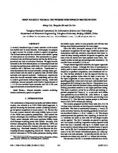
where E[·] represents the expectation operator. These parameters are learned from the spectral vector sequences representing a training corpus of clean speech. Since the process is assumed to be Gaussian, all unreliable spectral components in any noisy signal can, in principle, be jointly estimated using the bounded MAP procedure. In practice, however, it is equally effective and far more efficient to estimate jointly only the unreliable components in individual spectral vectors, based on the reliable components within a neighborhood enclosing the vectors. To estimate the unreliable components in the m th spectral vector X(m) we arrange them in a vector X u(m). We identify the set of all reliable spectral components in the spectrogram that have a normalized covariance of at least 0.5 with at least one of the elements in X u(m) and arrange them into a neighborhood (n) vector X r (m). Figure 2 illustrates the construction of the neighborhood vector. The joint distribution of X u(m) and (n) X r (m) is Gaussian. The expected values and the covariance (n) matrices of X u(m) and X r (m) and the cross covariance between them can all be constructed from the mean and covariance parameters of the underlying Gaussian process. Once the parameters of the joint Gaussian distribution of X u(m) and (n) X r (m) are constructed in this fashion, the true value of X u(m) is estimated using the bounded MAP estimation procedure. CLASSIFIER-MODIFICATION METHODS An alternative to estimating the true values of the unreliable or missing components is to modify the classifier itself to perform recognition with unreliable or incomplete data. The two most popular classifier-modification methods have been classconditional imputation [19] and marginalization [11]. With feature-imputation methods, recognition can be performed

using feature vectors that may be different from (and derived from) the spectral vectors that are reconstructed from the partially degraded input. In classifier-modification methods, however, recognition is usually performed using the spectral vectors themselves as features. CLASS-CONDITIONAL IMPUTATION In class-conditional imputation, state-specific estimates are derived for unknown spectral components, prior to estimating the state output density P(X|s). In other words, when computing the state output density value at any state s for any vector X, the unreliable components of X are estimated using the state output density of s. We assume that the output density of any state s is a Gaussian mixture, given by

P(X|s) =

ν

cs,ν (2π| s,ν |)− 2 e− 2 (X−µ s,ν ) d

1

−1 s,ν (X−µ s,ν )

where the subscript s applied to the parameters of the distribution indicates that they are specific to the output distribution of state s. As before, let Y be any observed spectral vector, with reliable and unreliable subvectors Yr and Yu . Let X represent the corresponding idealized clean vector and X r and X u its subvectors corresponding to Yr and Yu . The state output density of any state s is defined over the complete vector X = X r ∪ X u . In order to compute P(X|s) we obtain the statespecific estimate for X u, Xˆ s,u as Xˆ s,u =

ν

P(ν|X r, X u ≤ Yu)

× BM AP(X u|X r, X u ≤ Yu; µ s,ν , s,ν ),

S(1,1)

S(2,1)

S(3,1)

S(4,1)

S(1,2)

S(2,2)

S(3,2)

S(4,2)

S(1,3)

S(2,3)

S(3,3)

S(4,3)

S(1,4)

S(2,4)

S(3,4)

S(4,4)

[FIG2] Illustration of a hypothetical spectrogram containing four spectral vectors of four components each. Components shown in gray are considered to be unreliable. The blocks with the diagonal lines represent components with a normalized covariance of 0.5 or greater with either S(2, 2) or S(2, 3). To reconstruct unreliable components of the second vector using covariance-based reconstruction, X u (2) is constructed from S(2, 2) and S(2, 3), and X r(n) (2) is constructed from S(1, 2), S(1, 4), S(2, 1), S(2, 4), S(3, 2), and S(3, 3).

, (16)

(17)

using the cluster-based reconstruction technique in conjunction with the state output distribution of s. The complete vector Xˆ s = X r ∪ Xˆ s,u is then constructed (with the components arranged in appropriate order), and the state output density value of s is computed as P( Xˆ s|s). MARGINALIZATION The principle behind marginalization is to perform optimal classification (i.e., recognition) directly based on the observed values of the reliable and unreliable input data. As applied to HMM-based speech recognition systems, this implies that state output densities are now replaced by a term that computes ˆ P(X|s) = P(X r, −∞ ≤ X u ≤ Yu|s).

(18)

We assume that the state output density P(X|s) for state s is given by (16), and we further assume that all the Gaussians in the mixture density in (16) have diagonal covariance matrices. For any observed spectral vector Y, let R represent the set of


indices of the reliable components and U represent the indices of the unreliable components. In other words, Yr is composed of all components Y(k) such that k ∈ R, and Yu is composed of all ˆ Y(k) such that k ∈ U. It is easy to show that P(X|s) as defined by (18) is now given by

ˆ P(X|s) =

ν

cs,ν P(X r, −∞ ≤ X u ≤ Yu; µ s,ν , s,ν ),

(19)

where P(X r, −∞ ≤ X u ≤ Yu; µ s,ν , s,ν ) is given by (7). Note that if the damaged spectral components X u were assumed to be completely unknown (so that Yu did not provide any information that constrained X u), then the limits on the integral terms on the right hand side of (19) would be (−∞, ∞), and the integral terms would evaluate to 1.0, thereby marginalizing out the unreliable spectral components from the state output density entirely. On the other hand, if it were possible to provide tighter bounds on the true value of X u , the integral term could use them as limits instead of (−∞, Yu). IDENTIFICATION OF UNRELIABLE COMPONENTS The most difficult aspect of missing feature methods is the estimation of the spectrographic masks that identify unreliable spectral components. The estimation can be performed in multiple ways: we may either attempt to estimate the SNR of each spectral component to identify unreliable components, or we may attempt to classify unreliable components directly using some other criteria in place of SNR. In the latter case, spectrographic masks may either be estimated from Bayesian principles applied to a variety of measurements derived from the speech signal, or from perceptually-motivated criteria. We discuss all of these alternatives below. ESTIMATING SPECTROGRAPHIC MASKS BASED ON SNR To estimate the SNR of spectral components, an estimate of the power spectrum of the corrupting noise is required. Typically, the noise power spectrum is estimated from regions of the signal that are determined to not contain speech. For example, in Vizinho et al. [36], the first several frames of any utterance are assumed to be regions of silence and the average power spectrum of these frames is assumed to represent the power spectrum of the noise. Alternately, the noise power spectrum can be estimated continuously by a simple recursion, in order to track slowly-varying noise. The noise power spectrum is initialized to the average power spectrum of the initial few frames of the incoming signal. Any subsequent sudden increases in energy in the noisy speech signal are assumed to indicate the onset of speech, while regions in the speech whose energies fall below a given threshold are assumed to consist only of noise. Let Yp(m, k) and Np(m, k) represent the k th frequency band of the power spectra of the observed noisy speech and the noise respectively, in the m th analysis window. The estimated value of Np(m, k) is obtained as

Nˆ p(m, k) =

 (1 − λ) Nˆ p(m − 1, k) + λYp(m, k),    if Y (m, k) < β Nˆ (m, k) p

 Nˆ (m − 1, k),   p otherwise.

p

(20)

Typical values of λ and β are 0.95 and 2, respectively, and the value of λ can be manipulated to track slower or faster variations in the noise. Other noise estimation techniques [18] may also be used in lieu of (20). Multiple criteria have been proposed to identify unreliable spectral components from the estimated noise spectrum. El-Maliki and Drygajlo [15] propose a negative energy criterion in which a spectral component is assumed to be unreliable if the energy in that component is less than the estimated noise energy in it. In other words Yp(m, k) is assumed to be unreliable if |Yp(m, k)| ≤ | Nˆ p(m, k)|.

(21)

The SNR criterion, on the other hand, identifies spectral bands as unreliable if the estimated SNR of any spectral component lies below 0 dB. To estimate the SNR, an estimate of the power spectrum of clean speech is required. This is obtained by spectral subtraction, i.e., by subtracting the estimated power spectrum of the noise from the power spectrum of the noisy speech signal as follows [7]:  Yp(m, k) − Nˆ p(m, k),    if Yp(m, k) − Nˆ p(m, k) > γ Yp(m, k) Xˆ p(m, k) =  (m, k), γ Y   p otherwise, (22) where Xˆ p(m, k) represents the estimate of the k th spectral component of the power spectrum of the clean speech signal in the m th analysis window. The parameter γ is a small flooring factor meant to ensure that the estimated power spectrum for the clean speech does not go negative. The SNR criterion states that a spectral component Yp(m, k) is to be assumed unreliable if the estimated power spectrum of the underlying clean speech is lower than the power spectrum of the noise, i.e., if Xˆ p(m, k) < Nˆ p(m, k). Alternately stated, Yp(m, k) is deemed unreliable if less than half the energy in Yp(m, k) is attributable to speech, i.e., if Xˆ p(m, k) < 0.5Yp(m, k).

(23)

In practice, the best mask estimates are obtained when both the negative energy criterion of (21) and the SNR criterion of (23) are used to identify unreliable spectral components. Figure 3(b) shows an example of a spectrographic mask obtained by noise estimation. In general, noise-estimate-based estimation of spectrographic masks may be expected to be


above, for voiced regions of speech, an additional feature is derived that measures the ratio of the energy of the signal at all harmonics of the pitch frequency that lie within the k th frequency band [for a location (m, k)], to the energy in frequencies between the pitch harmonics. The pitch estimate required by this feature is obtained with a pitch estimation algorithm. Separate classifiers are trained for voiced and unvoiced speech, and for each frequency band, using training data for which the true spectrographic masks are known (e.g., clean speech signals that have been digitally corrupted by noise). All distributions are modeled as a mixture of Gaussians, the parameters of which are learned from the feature vectors of appropriately labeled spectral components of the training data (e.g., the distribution of reliable voiced components in the k th frequency band is learned from the feature vectors of reliable components in the k th frequency band of voiced portions of the training data). The a priori probabilities of the reliable and unreliable classes for each classifier are also learned from training data. During recognition, noisy speech recordings are first segregated into voiced and unvoiced segments (typically using a pitch detection algorithm; segments where it fails to estimate a reasonable pitch value are assumed to be unvoiced). The appropriate feature vectors are then computed for each time-frequency location. The (m, k)th time-frequency location is classified as reliable if

effective when the corrupting noises are stationary or pseudostationary. For nonstationary and transient noises, however, the estimation of the noise spectrum is difficult and this technique can result in highly inaccurate spectrographic masks.

20 18 16 14 12 10 8 6 4 2

PV,k(reliable)PV,k(F(m, k)|reliable) > PV,k(unreliable)PV,k(F(m, k)|unreliable)

20 18 16 14 12 10 8 6 4 2 0.5

1 1.5 Time (s) (a)

2

2.5

0.5

(24)

where F(m, k) is the feature vector for (m, k), V is a voicing tag that indicates whether F(m, k) belongs to a voiced segment or not, PV,k(reliable) represents the a priori probability that the k th frequency component of a spectral vector with voicing tag V is reliable, and PV,k(F|reliable) represents the distribution of feature vectors of reliable components in the k th frequency band of speech segments with voicing tag V.

Mel Filter Index

Mel Filter Index

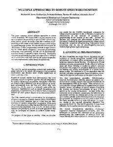
BAYESIAN ESTIMATION OF SPECTROGRAPHIC MASKS The Bayesian approach to estimating spectrographic masks treats the tagging of spectral elements as reliable versus unreliable as a binary classification problem. Renevey et al. [31] use estimates of the distribution of noise to compute an explicit probability that the noise energy in any spectral component exceeds the speech energy in it. In this article, however, we describe an alternative technique presented by Seltzer et al. [35] that does not depend entirely on explicit characterization of the noise. Here, a set of features is computed for every time-frequency location of the spectrogram. Features are designed that exploit the characteristics of the speech signal itself, rather than measurements of the corrupting noise. These features are then input to a conventional Bayesian classifier to determine whether a specific time-frequency component is reliable. We note that each time-frequency location in the spectrogram actually represents a window of time and a band of frequencies. The features extracted for any time-frequency location are designed to represent the characteristics of the signal components within the corresponding frequency band, in the given window of time. The features for any time-frequency location (m, k) include 1) the ratio of the first and second autocorrelation peaks of the signal within that window, 2) the ratio of the total energy in the k th frequency band to the total energy of all frequency bands, 3) the kurtosis of the signal samples within the mth frame of speech, 4) the variance of the spectrographic components adjoining (m, k), and 5) the ratio of the energy within Yp(m, k) to the estimated energy of the noise Np(m, k). The noise estimate is obtained using the procedure outlined in (20). Note that the estimated SNR is only one of the features used and is not the sole determinant of reliability. In addition to the features described

1 1.5 Time (s)

2

20 18 16 14 12 10 8 6 4 2

2.5

(b)

0.5

1 1.5 Time (s)

2

2.5

(c)

[FIG3] (a) An ideal spectrographic mask for an utterance corrupted to an SNR of 10 dB by white noise. Reliable time-frequency components have been identified based on their known SNR. An SNR threshold of 0 dB has been used to generate this mask. (b) Spectrographic mask for the same utterance obtained by estimating the local SNR of the signal. (c) Spectrographic mask obtained by using Bayesian classification.


Word Accuracy (%)

Word Accuracy (%)

reliable time-frequency regions in a representation of a complex Figure 3(c) shows an example of a spectrographic mask auditory scene that are believed to arise from a common obtained using the Bayesian approach. We observe that the azimuth. By passing these reliable components to a missing feaBayesian mask is superior to the noise-estimate-based mask ture recognizer similar to the in this example. In general, fragment decoder described since Bayesian mask estimaTHE ACCURACY OF AUTOMATIC below, Palomaki et al. have tion is not strictly dependent SPEECH RECOGNITION SYSTEMS demonstrated that the use of on the availability of good IS STILL ADVERSELY AFFECTED cues extracted using binaural estimates of the noise specBY NOISE AND OTHER SOURCES processing can lead to a very trum (as the estimated SNR OF ACOUSTICAL VARIABILITY. substantial improvement in is only one of the features speech recognition accuracy used), it is effective both for when the target speech signal and interfering signals arrive stationary and nonstationary noises. For example, Seltzer et from different azimuths. al. [35] report that effective spectrographic masks can be Spectrographic masks that are derived from perceptual prinderived using the Bayesian approach for speech corrupted by ciples are based entirely on the known structural patterns of music, whereas masks derived from noise estimates are totalspeech spectra and are not dependent on noise estimates in any ly ineffective. Nevertheless, Bayesian mask estimation may be manner. As a result, this approach can result in effective specexpected to fail when the spectral characteristics of the noise trographic masks even in very difficult environments, e.g., in are similar to those of speech, such as when the corrupting the presence of competing speech signals. signal is speech from a competing speaker. The Bayesian mask also has the advantage that the classifier computes the DEALING WITH UNCERTAINTY IN MASK ESTIMATION probability of unreliability P(unreliable|F(m, k)). These probRegardless of the actual technique employed, it is never possible abilities can be used in conjunction with the soft-mask techto identify unreliable spectral components with complete cernique described later in this article. tainty. Errors in the spectrographic mask can cause the recognition performance of missing feature methods to degrade MASK ESTIMATION FROM PERCEPTUAL CRITERIA significantly. Figure 4 describes the recognition accuracy This approach attempts to identify groups of speech-like spectral obtained with various missing feature methods, comparing the components based on the physics of sound and selected properaccuracy obtained using oracle spectrographic masks (that are ties of the human auditory system. For example, in voiced obtained with knowledge of the true SNR of the spectral compospeech, most of the energy tends to occur around the harmonics nents) to the accuracy obtained using masks that were estimated of the fundamental frequency. Barker et al. [4] propose that blindly from the incoming data. The degradation in recognition within each frame of speech that is identified as voiced and has a valid pitch estimate, all time-frequency components that occur at the 70 90 harmonics of the pitch 80 may be assumed to be 60 reliable and represent 70 50 speech. Such masks, Matched 60 Ideal however, have been 40 50 Estimated found to be most effecBaseline 40 30 tive when used in con30 junction with other 20 20 masks, such as noise10 10 estimate based masks; 0 0 any spectral component 0 5 10 15 20 25 0 5 10 15 20 25 that is identified as reliSNR (dB) SNR (dB) able by either mask is assumed to be reliable. (a) (b) Palomaki et al. [24] have described a binaural [FIG4] Recognition accuracy for speech corrupted by white noise as a function of SNR using two different missing feature methods. (a) Recognition accuracy obtained using marginalization. Recognition is processing model that performed using log-spectral vectors. (b) Recognition accuracy obtained using cluster-based reconstruction. extracts information Recognition is performed with cepstral vectors derived from reconstructed spectrograms. In both panels, about interaural time the triangular symbols show recognition performance obtained with ideal spectrographic masks, while the diamonds show recognition accuracy with estimated spectral masks. The square symbols show the delays and intensity dif- recognition accuracy of a matched recognizer that had been trained in the testing environment, while the ferences to identify the delta symbols at the bottom show the accuracy obtained when the recognizer is trained with clean speech.


accuracy due to errors in mask estimation is evident. We have observed that erroneous tagging of reliable components as being unreliable degrades recognition accuracy more than tagging unreliable elements as reliable. More detailed analyzes of the effects of mask estimation errors may be found in [28] and [35]. Two different remedies have been proposed to cope with the effects of mask estimation errors. In the first approach, soft masks are estimated that represent the probability that a given spectral component is reliable (as opposed to a binary mask that unambiguously tags spectral components as reliable or unreliable). In the second approach, the mask estimation is performed as a part of the speech recognition process itself, with the expectation that the detailed and precise statistical models for speech that are used by the recognizer will also enable more accurate estimation of masks. SOFT MASKS Under the soft-decision framework, each spectral element Y(m, k) is assigned a probability γ = P(reliable|Y(m, k)) that it is reliable and dominated by speech rather than noise. The probability of reliability is arrived at differently by different authors. The Bayesian mask estimation algorithms of Seltzer et al. [35] and Renevey et al. [31] can be used to obtain γ directly. Barker et al. [6] employ an alternate approach, approximating γ as a sigmoidal function of the estimated SNR of Y(m, k).

γ ≈

1 . 1 + exp(−α(SNR(m, k) − β))



k

−(Y( j)−µ s,k ( j))2

ˆ Sˆ = arg max{P(W, S|Y)} W, W,S

P(X|S, Y) ˆ Sˆ = arg max P(W) W, dX P(S|Y) P(X|W) P(X) W,S (28) where P(S|Y) represents the probability of spectrographic mask S given the noisy spectral vector sequence Y, which is assumed to be independent of the word sequence W. In practical implementations of HMM-based speech recognition systems, the optimal state sequence is determined along with the best word sequence. The corresponding modification to (27) used by the speech fragment decoder is

ˆ Sˆ = arg max max W, W,S

m

0

Y(l)

−(x−µ s,k (l))2

(27)

where S represents any spectrographic mask and Sˆ represents the optimal mask, and Y represents the entire spectral vector sequence for the noisy speech. Letting X be the ideal spectral vector sequence for the clean speech underlying Y, this can be shown to be equal to

×

j

2σ s,k ( j) (1 − γ )  e + × γ Y(l) 2πσ s,k( j)

SIMULTANEOUS RECOGNITION AND MASK ESTIMATION Possibly the most sophisticated missing feature technique is the speech fragment decoder proposed by Barker et al. [3], [5]. In the speech fragment decoder the search mechanism used by the speech recognizer is modified to derive the optimal spectrographic mask jointly with the optimal word sequence. In order to do this, the Bayesian classification equation given in (5) is modified to become

(25)

The SNR itself is estimated from the estimated differences in level between speech and noise, using the procedures described previously. Typical values for α and β are 3.0 and 0.0, respectively. Morris et al. [22] show that marginalization based on soft masks can be implemented with a relatively minor modification to the bounded marginalization algorithm of (19) for HMMbased speech recognition systems that model state output densities as mixtures of Gaussians with diagonal covariance matrices: P(Y|s) =

feature technique that can utilize soft masks effectively, since other techniques require unambiguous identification of unreliable spectral components.



e 2σ s,k ( j)  dx . 2πσ s,k(l) (26)

Note that in (26) Y(l ) is the l th component of Y; (26) is equivalent to a model that assumes that spectral features are corrupted by a noise process that leaves them unchanged with a probability γ , or with a probability 1 − γ adds to them a random value drawn from a uniform probability distribution in the range (0, Y(l )). We also note that marginalization is the only missing

s

  

P(S|Y)P(W)P(s|W)

  P(X(t)|S, Y) dX(m) . (29) P(X(t)|sm )  P(X(m))

Here s represents a state sequence through the HMM for W, sm represents the mth state in the sequence, P(s|W) represents the a priori probability of s and is obtained from the transition probabilities of the HMM for W, X(m) represents the mth vector in X, and P(X|s) represents the state output density of s. Let S(m) represent the spectrographic mask vector for Y(m). Let U(m) represent the set of spectral components of Y(m) that are tagged as unreliable (or, alternately, as belonging to the background noise) by S(m). Let R(m) be the set of frequency bands that are identified as reliable. Let Y(m, j) and X(m, j) represent the j th component of Y(m) and X(m),


respectively. All state output densities are modeled as mixtures of Gaussians with diagonal covariance matrices, as given by (16). By further assuming that the conditional probabilities P(X(m, j)|S, Y ) are independent for the various values of j, and that P(X(m, j)|S, Y ) is 0 for X(m, j) > Y(m, j) and proportional to P(X(m, j)) otherwise, and finally that the a priori probability of X(m, j) is a uniform density between 0 and xmax , the acoustic probability term within the parentheses on the right hand side of (29) is computed as

P(X(m)|S, Y) dX(m) P(X(m)) −(Y(m, j)−µ s,k ( j))2 2σ s,k ( j) e

P(X(m)|sm ) =

cst,k

k

l∈U(m) 0

j∈R(m) Y(m,l)

e

−(x−µ s,k ( j))2 2σ s,k ( j)

xmax dx Y(m, l)

(30)

A complete implementation of (29) requires exhaustive evaluation of every possible spectrographic mask and is computationally infeasible. Instead, the fragment decoder hypothesizes a large number of fragments or regions of the spectrogram within which all components are assumed to belong together. Fragments may be hypothesized based on various criteria including SNR and acoustic cues such as harmonicity. Joint recognition and search for the optimal spectrographic mask is performed only over spectrographic masks that may be formed as combinations of these fragments. Barker et al. implement this procedure using a token-passing algorithm that is described in [3]. The fragment-decoding approach has been shown by Barker et al. to be more effective than simple bounded marginalization. It also has the advantage over other missing feature methods that it can be easily extended to recognize multiple mixed signals, such as those obtained from the combined speech of multiple simultaneous talkers. The only requirement is that the precomputed fragments group spectral components from a single speaker accurately. ADDITIONAL PROCESSING OF SPECTRAL INPUT The discussion thus far has assumed implicitly that recognition is performed directly using the incoming spectral vectors as features. However, most speech recognizers preprocess incoming feature vectors in various ways in order to improve recognition accuracy. For example, recognizers usually use cepstra derived from log spectral vectors, rather than the log-spectral vectors themselves, because cepstral vectors are known to result in significantly greater accuracy [13]. Recognition systems that use feature-vector imputation can work from cepstral vectors since these can be derived from the complete spectral vectors reconstructed by this approach. On the other hand, classifiermodification methods are generally ineffective for recognizers that work from cepstral vectors, since they require information that characterizes the reliability of each component of the

incoming feature vectors, and such information is available only for spectral vectors. Other common types of preprocessing of incoming feature vectors include augmentation using difference vectors and mean normalization of feature vectors. Again, while these manipulations do not pose problems for feature-vector reconstruction methods, classifier-modification methods must be modified to accommodate them, and they in turn constrain the specific missing feature methods that can be employed. TEMPORAL-DIFFERENCE FEATURES In most recognizers, the basic feature vector at any time is augmented by difference and double-difference vectors. Difference vectors represent the trend, or velocity, of the feature vectors and are usually obtained as the difference between adjacent feature vectors. The use of this information partially compensates for the commonly used but clearly inaccurate assumption that features extracted from successive analysis frames are statistically independent. The difference vector for frame m is obtained as D(m) = Y(m + ξ ) − Y(m − ξ )

(31)

where D(m, k), the k th component of D(m) becomes unreliable if either Y(m + ξ, k) or Y(m − ξ, k) is unreliable. Double difference vectors represent the acceleration of the spectral vectors and are computed as the difference between adjacent difference vectors: DD(m) = D(m + ζ ) − D(m − ζ )

(32)

DD(m, k) is unreliable if either D(m + ζ, k) or D(m − ζ, k) is unreliable. In the worst case, difference vectors may have as much as twice as many unreliable components on average as the spectral vectors, while double difference vectors may have up to four times as many unreliable components. In practice, however, unreliable components tend to occur in contiguous patches, and the fraction of components in the difference and double difference vectors that are unreliable tends not to be much greater than those of the spectral vectors themselves. The upper and lower bounds on the values of unreliable difference and double difference vector components must be computed from the bounds on (or values of) the spectral components of which they are composed. For methods that use soft masks, the reliability probability of these terms must also be derived from the reliability probabilities of the spectral components from which they were computed. MEAN NORMALIZATION Mean normalization [2] refers to the procedure by which the mean feature vector of any sequence of feature vectors is subtracted from all vectors in the sequence, so that the resulting


sequence has zero mean. In symbolic terms, the mth normal¯ ized vector Y(m) of any sequence of feature vectors Y(1), Y(2), . . . , Y(M) is computed as

on all aspects of the problem, it is not possible to identify a consistent set of results that have all been obtained on the same systems and databases. Consequently, the experimental results we present in this article have been culled from a number of papers and sources. We have attempted to maintain a modicum 1 ¯ Y(m) = Y(m) − Y(m). (33) of consistency where possible; most of the results described M m have been obtained from experiments conducted in the authors’ laboratory at Carnegie Mellon University (CMU). The CMU experiments were conducted using the Resource Mean normalization is commonly observed to result in large Management database [26], with the Sphinx-3 HMM-based improvements in the recognition accuracy of automatic speech recognition system, speech recognitions systems. with 2,000 tied state distribuUnfortunately, mean normalMISSING FEATURE METHODS MODEL tions with Gaussian state outization as described by (33) THE EFFECTS OF NOISE ON SPEECH put densities. We have mainly cannot be performed with presented results for speech classifier-modifying missing AS THE CORRUPTION OF REGIONS corrupted by white noise, feature methods because OF TIME-FREQUENCY although similar results have many components of the feaREPRESENTATIONS OF THE also been obtained using ture vectors used for recogniSPEECH SIGNAL. other noise types. Other tion are potentially results reported in this article unreliable. The mean value have been drawn from experiments conducted at the University of all vectors, as used in (33), would include the contributions of Sheffield and elsewhere, using the TI digits database. Where of these unreliable components and would be unreliable itself, we report such results, the details of the experimental setup and normalization by such a mean estimate results in degradaused for the experiments have been provided. tion of recognition performance [30]. Alternately, the mean Speech is a highly redundant signal, with the evidence for value could be computed from only the reliable components of any acoustic event being multiply represented in several frethe spectrogram. Unfortunately, the reliable regions of specquency bands, often over several tens of milliseconds of time. trograms contain chiefly high-energy spectral components, Raj et al. [28] report that speech recognition performance does and mean estimates obtained from them tend to be biased, not degrade significantly when a randomly selected 80% of the again resulting in degraded recognition performance. elements are excised from a spectrogram and recognition is perA useful substitute for mean normalization has been proformed with only the remaining elements. Similar results have posed by Palomaki et al. [25]. Instead of subtracting the mean been reported by other researchers, e.g., Cooke et al. [9]. The value of the spectral vector, every spectral component is normissing feature approach therefore promises to be highly effecmalized by a value that represents the upper percentile of the ¯ k), the tive for noise-robust speech recognition. Traditionally, the best values for that component. Using this approach, Y(m, strategy to recognize speech that has been corrupted by stationnormalized value of Y(m, k), is computed as ary noise has been to train a matched recognizer with speech 1 that had been corrupted to the same level by the same kind of ¯ Y(m, k) = Y(m, k) − Y(τ, k) (34) noise. Figure 4(a) and (b) compares the recognition accuracy D τ ∈L obtained using matched recognizers on speech corrupted to various SNRs by white noise, with the performance obtained with where L represents the set of frame indices of the D greatest Y(m, k) values that are reliable. Palomaki et al. [25] observe two different missing feature methods using ideal spectrographic masks that had been derived with perfect knowledge of the that five is a good value for D, although lower values are also true SNR of every spectrographic element, as well as using receffective. This approach has the advantage that the normalizaognizers that had been trained with clean speech. The recognition term does not get biased by the presence of unreliable comtion accuracy performance obtained with the missing feature ponents in the spectrum. Thus, the normalization given by [34] method is observed to be comparable to that obtained with a can be effectively used with missing feature methods. matched recognizer. In practice, spectrographic masks must be estimated, and EXPERIMENTAL RESULTS AND DISCUSSION the recognition accuracy obtained with estimated masks (also In this section we discuss and compare various aspects of missshown in Figure 4) is significantly worse than that obtained ing feature methods and their relative merits. Where possible, using ideal masks. Nevertheless, missing feature methods have we present experimental evidence in support of our statements. the advantage that the recognizer need not be retrained for We note that missing feature methods remains an active area of every noise type or level, and they also hold the promise that research and that the techniques presented in this article have the performance could improve significantly with improved been developed by a number of people from a variety of mask estimation. More importantly, matched recognizers canresearch groups. Since not all of these researchers have worked


tion. Consequently the best recognition accuracy can be expected not be trained for most practical situations, since the level and from marginalization. Unfortunately, marginalization has the characteristics of the noise change even within the course of disadvantage that recognition must be performed with spectral an utterance. Instead, multistyle recognizers are trained that vector sequences directly. In general, however, recognition accuattempt to strike an effective compromise across all the racy obtained with cepstral vectors derived from spectral vectors observed noise types and levels. Experiments reported by is much superior to that obtained with spectral vectors. FeatureBarker et al. [4] (Figure 5) show that missing feature methods imputation methods that reconstruct entire spectrograms can outperform such recognizers even when the spectrographenable recognition with cepstral vectors derived from the reconic masks are estimated. structed spectrograms. The benefits of going to the cepstral As noted earlier, highly nonstationary noises such as music domain often overcome the advantage gained by the optimal pose special problems for speech recognition systems. classification performed with Conventional noise compensaspectral vectors in marginaltion schemes are rendered THE MOST DIFFICULT ASPECT OF ization, especially at high ineffective by such noises. MISSING FEATURE METHODS IS THE SNRs. This is demonstrated in However, missing feature Figure 7, which compares methods have been shown to ESTIMATION OF THE SPECTROGRAPHIC recognition performance result in significant improveMASKS THAT IDENTIFY UNRELIABLE obtained with spectral and ments in recognition accuracy SPECTRAL COMPONENTS. cepstral vectors using various even on such noises (Figure 6). missing feature methods. Not all missing feature Figure 7 and other results reported in the literature also methods are equivalent and useful in all situations, however, shows that class-conditional imputation and covariance-based and different implementations have different characteristics. reconstruction generally result in much poorer recognition The SNR threshold that is used to determine which signal comthan either marginalization or cluster-based reconstruction. ponents are unreliable is typically higher for classifier-modificaHowever, these methods do have their uses. For example, tion methods than for feature-imputation methods. For missing Josifovski et al. [19] report that class-conditional imputation is feature methods with relatively low SNR thresholds for unreliahighly effective for reconstruction of complete spectrograms bility, even spectral components tagged as reliable often have a from partial or unreliable ones. Raj et al. [28] show that when certain degree of noise. For such methods, reducing the noise spectrographic components are lost due to random deletions level in these components using a technique such a spectral (e.g., due to loss during transmission), covariance-based reconsubtraction improves recognition accuracy [28]. For methods struction, which draws on information from adjacent vectors to for which the SNR threshold for reliability is relatively high, reconstruct any missing component, is by far the best spectrospectral subtraction does not greatly improve accuracy. gram reconstruction method. Of the various missing feature methods, only marginalization and its derivative algorithms (soft-mask marginalization and fragment decoding) purport to perform optimal classifica80

100

Word Accuracy (%)

80 60 Marginalization Multistyle

40

Word Accuracy (%)

70 60 50 40 30 Cluster–Based Estimation

20

Baseline

10

Baseline

0

20

0

5

10

15

20

25

SNR (dB) 0

−5

0

5

10 15 SNR (dB)

20

Clean

[FIG5] Comparison of recognition accuracy obtained using multistyle training and with soft-mask marginalization. The experiment was conducted on Test Set A of the Aurora corpus. Recognition was performed with spectral vectors.

[FIG6] Recognition accuracy for speech corrupted by music. The spectrographic mask was estimated using a Bayesian classifier, and unreliable components were reconstructed by cluster-based reconstruction. Recognition was performed using cepstra derived from reconstructed spectrograms. The lower curve shows the recognition accuracy obtained when no missing feature methods were used. The RM database was used for this experiment, and the recognizer was trained with clean speech.


tion method for the reasons discussed earlier. Cooke and his colleagues have suggested that the difference between the recognition accuracy obtained with spectral and cepstral vectors may be greatly reduced (although perhaps not eliminated) by using more detailed state output distributions for the HMMs. They have also noted that cepstral vectors are intrinsically able to provide a greater degree of normalization for level and spectral tilt than log-spectral features computed without mean normalization. A serious problem for missing feature methods is that mask estimation 100 70 is an unreliable process, 60 80 and estimated masks are 50 often errorful. Of all the 60 40 missing feature meth30 40 ods, marginalization is 20 the most robust to mask 20 estimation errors. The 10 soft-mask variant of 0 0 marginalization 0 5 10 15 20 25 0 5 10 15 20 25 described previously can SNR (dB) SNR (dB) result in greater robust(a) (b) ness to uncertainty in mask estimation, as [FIG7] Recognition accuracy obtained with various missing feature methods on speech corrupted by demonstrated by the white noise. (a) shows the performance obtained with classifier-modification methods on a recognizer results in Figure 8 that works with spectral vectors. Recognition accuracy is obtained using marginalization (square symbols) and state-based imputation (triangles). (b) shows recognition performance obtained with cepstra derived obtained by Barker et al. from spectrograms reconstructed by the feature-imputation methods of cluster-based imputation (circles) [6]. The fragment deand correlation-based imputation (stars). These results are compared with results obtained using front coder described previends that do not perform missing feature analysis: spectral subtraction (diamonds), and baseline performance (deltas). ously is, in principle, the Word Accuracy (%)

Word Accuracy (%)

In considering the data in Figure 7 it should be noted that the relatively poor recognition results obtained using spectral coefficients may be partially accounted for by the fact that recognition was performed using 20-dimensional log-spectral features, with single-Gaussian HMM output distributions and no cepstral mean normalization or similar processing. Cepstral mean normalization was not employed in these experiments because it cannot be meaningfully applied for the marginaliza-

100 100 80 Word Accuracy (%)

Word Accuracy (%)

90 80 70 "Soft" Mask 60

"Hard" Mask Baseline

50

60 Fragment Decoder 40

"Hard" Mask Baseline

20

40 0 30

0

5

10

15

20

0

5

25

10

15

20

25

SNR (dB)

SNR (dB) [FIG8] Comparison of recognition accuracy obtained using softmask marginalization (squares) with the accuracy obtained using conventional bounded marginalization (triangles) on speech corrupted by Lynx helicopter noise. The TI digits corpus has been used for this experiment. Recognition was performed with spectral vectors. The baseline performance obtained without missing-feature methods is also shown.

[FIG9] Comparison of recognition accuracy obtained by fragment decoding (squares) with that obtained by bounded marginalization (triangles). Recognition was performed with spectral vectors for both missing feature methods. Baseline recognition accuracy with mel frequency cepstral coefficients, using cepstral mean normalization, is also shown. The TI-digits database was corrupted by noise samples from the NOISEX database for this experiment.


optimal method for mask estimation since it actually uses the recognizer itself to identify the best mask and can result in significant improvements over the recognition accuracy obtained when spectrographic masks are computed separately from the recognizer. Typical results are illustrated in Figure 9, using data provided by Barker et al. [3]. In practice, its performance is limited by the accuracy of the hypothesized fragments that are themselves obtained using other, potentially errorful techniques. These errors can be reduced by hypothesizing smaller fragments with greater likelihood of consistency, at the cost of increased computation. The inability to perform additional processing such as mean subtraction has sometimes been considered a problem for classifier-modification-based missing feature methods. Nevertheless, the technique proposed by Palomaki et al. [25] described previously provides a good substitute for CMN that can be used with missing feature methods. Unfortunately, no mechanism has been developed to take advantage of either this technique or difference vectors for soft-mask methods or fragment decoders. The dramatic and consistent success enjoyed by the missing feature techniques described in this article may cause one to question why these approaches have not been widely employed in state-of-the-art large vocabulary continuous speech recognition (LVCSR) systems such as those developed for the Defense Advanced Research Projects Agency (DARPA) Broadcast News and Switchboard tasks. While there are probably a number of reasons for this (including the observations that some algorithms are somewhat computationally costly and that the field has only stabilized significantly in recent years), it is certainly the case that the speech signals encountered in tasks like Broadcast News and Switchboard are more degraded by the effects of speaking style and disfluencies in speech production than they are by background noise. We expect that missing feature techniques will be employed much more widely in tasks for which there is significant degradation due to noise and especially if the sources in noise are nonstationary or transient in nature. A final topic that has not been explored significantly is the issue of training with noisy data. Conventional recognizers have benefited greatly when they have been trained with the kind of noisy speech that they are expected to recognize. Missing feature methods, on the other hand, are usually developed within the paradigm of training the recognizer with clean data. It is likely that the performance of these methods would improve further if the recognizer itself has been trained with incomplete or unreliable spectrograms obtained from noisy speech. While the mathematics of such a training procedure are well known, the topic itself remains to be explored. SUMMARY In this article we have reviewed a wide variety of techniques based on the identification of missing spectral features that have proved effective in reducing the error rates of automatic speech recognition systems. These approaches have been con-

spicuously effective in ameliorating the effects of transient maskers such as impulsive noise or background music. We described two broad classes of missing feature algorithms: feature-vector imputation algorithms (which restore unreliable components of incoming feature vectors) and classifiermodification algorithms (which dynamically reconfigure the classifier itself to cope with the effects of unreliable feature components). We reviewed the mathematics of four major missing feature techniques: the feature-imputation techniques of cluster-based reconstruction and covariance-based reconstruction, and the classifier-modification methods of classconditional imputation and marginalization. We then considered the very difficult task of estimating the spectrographic masks that identify which components of incoming spectral vectors are unreliable, focusing on the estimation of spectrographic masks from estimates of statistical parameters that represent characteristics of the noise, as well as Bayesian estimation methods that typically exploit characteristics of the speech to be recognized. We concluded our discussion of spectrographic masks with a description of how uncertainty in the estimation can be incorporated into the recognition process, describing soft-mask techniques, and fragment-decoding systems that simultaneously recognize the spectrographic masks and the incoming spoken utterance. We also discussed the ways in which the common feature extraction procedures of cepstral analysis, temporal-difference features, and mean subtraction can be handled by speech recognition systems that make use of missing feature techniques. We concluded with a discussion of a small number of selected experimental results. These results confirm the effectiveness of all types of missing feature approaches discussed in ameliorating the effects of both stationary and transient noise, as well as the particular effectiveness of both soft masks and fragment decoding. ACKNOWLEDGMENTS We are extremely grateful to Mike Seltzer for his help and advice in many aspects of this work and to Martin Cooke and Jon Barker for permission to use some of their experimental data. We also thank Martin Cooke and Dan Ellis for many helpful comments and suggestions in the review process. The work described was sponsored by the Space and Naval Warfare Systems Center, San Diego, under Grant N66001-99-1-8905. Preparation of the manuscript is partially supported by the Mitsubishi Electric Research Laboratories and by the National Science Foundation (Award IIS 0420866). AUTHORS Bhiksha Raj received the Ph.D. degree in electrical and computer engineering from Carnegie Mellon University, Pittsburgh, Pennsylvania, in May 2000. Since 2001, he has been working at Mitsubishi Electric Research Laboratories, Cambridge, Massachusetts. He works mainly on algorithmic aspects of speech recognition, with special emphasis on improving the robustness of speech recognition systems to environmental noise. His latest work was on the use of statistical information


encoded by speech recognition systems for various signal processing tasks. He is a Member of the IEEE. Richard M. Stern received the S.B. degree from the Massachusetts Institute of Technology (1970), the M.S. degree from the University of California, Berkeley (1972), and the Ph.D. from MIT (1977), all in electrical engineering. He has been on the faculty of Carnegie Mellon University since 1977, where he is currently a professor in the Electrical and Computer Engineering, Computer Science, and Biomedical Engineering Departments and the Language Technologies Institute. Much of his current research is in spoken language systems. He is particularly concerned with the development of techniques to make automatic speech recognition more robust with respect to changes in environmental and acoustical ambience. He has also developed sentence parsing and speaker adaptation algorithms for earlier CMU speech systems. In addition to his work in speech recognition, he also maintains an active research program in psychoacoustics, where he is best known for theoretical work in binaural perception. He is a Member of the IEEE and the Acoustical Society of America, and he was a recipient of the Allen Newell Award for Research Excellence in 1992.

[18] H.G. Hirsch and C. Ehrlicher, “Noise estimation techniques for robust speech recognition,’’ in Proc. IEEE Conf. Acoustics, Speech Signal Processing, Detroit, Michigan, 1995, pp. 153–156.

REFERENCES

[23] P.J. Moreno, “Speech recognition in noisy environments,” Ph.D. dissertation, ECE Dept., Carnegie Mellon Univ., Pittsburgh, PA, May 1996.

[1] S. Ahmed and V. Tresp, “Some solutions to the missing feature problem in vision,” in Advances in Neural Information Processing Systems 5. San Mateo, CA: Morgan Kauffman, 1993, pp. 393–400. [2] B.S. Atal, “Effectiveness of linear prediction characteristics of the speech wave for automatic speaker identification and verification,’’ J. Acoust. Soc. Amer., vol. 55, no. 6, pp. 1304–1312, 1974. [3] J. Barker, M.P. Cooke, and D.P.W. Ellis, “Decoding speech in the presence of other sources,’’ Speech Commun., vol. 45, no. 1, pp. 5–25, 2005. [4] J. Barker, M. Cooke, and P. Green, “Robust ASR based on clean speech models: An evaluation of missing data techniques for connected digit recognition in noise,” in Proc. Eurospeech-2001. Aalborg, Denmark: 2001, pp. 213–216. [5] J. Barker, M. Cooke, and D. Ellis, “Combining bottom-up and top-down constraints for robust ASR: The multisource decoder,” in Proc. Workshop Consistent Reliable Acoustic Cues (CRAC), Sept. 2001. [6] J. Barker, L. Josifovski, M. Cooke, and P. Green, “Soft decisions in missing data techniques for robust automatic speech recognition,” in Proc. ICSLP 2000, Beijing, China, Sept. 2000, pp. 373–376. [7] S. Boll, “Suppression of acoustic noise in speech using spectral subtraction,’’ IEEE Trans. Acoust. Speech Signal Processing, vol. 27, no. 2, pp. 113–120, 1979. [8] M.P. Cooke and D.P.W.E. Ellis, “The auditory organization of speech and other sources in listeners and computational models,’’ Speech Commun., vol. 35, no. 3–4, pp. 141–177, 2001. [9] M.P. Cooke, P.G. Green, and M.D. Crawford, “Handling missing data in speech recognition,” in Proc. ICSLP-1994, Yokohama, Japan, 1994, pp. 1555–1558. [10] M.P. Cooke, A. Morris, and P.D. Green, “Missing data techniques for robust speech recognition,” in Proc. IEEE Conf. Acoustics, Speech, Signal Processing, Munich, Germany, 1997, pp. 863–866.

[14] A.P. Dempster, N.M. Laird, and D.B. Rubin, “Maximum likelihood from incomplete data via the EM algorithm,” J. Royal Stat. Soc., vol. 39, no. 1, pp. 1–38, 1977. [15] M. El-Maliki and A. Drygajlo, “Missing features detection and handling for robust speaker verification,’’ in Proc. Eurospeech 1999, Budapest, Hungary, pp. 975–978. [16] B.J. Frey, L. Deng, A. Acero, and T. Kristjansson, “ALGONQUIN: Iterating LaPlace’s method to remove multiple types of acoustic distortion for robust speech recognition,’’ in Proc. Eurospeech 2001, Aalborg, Denmark, 2001, pp. 901–904. [17] H. Fletcher, Speech and Hearing in Communication. New York: Van Nostrand, 1953.

[19] L. Josifovski, M. Cooke, P. Green, and A. Vizihno, “State based imputation of missing data for robust speech recognition and speech enhancement,’’ in Proc. Eurospeech, Budapest, Hungary, 1999, pp. 2837–2840. [20] R.P. Lippmann and B.A. Carlson, “Using missing feature theory to actively select features for robust speech recognition with interruptions, filtering and noise,’’ in Proc. Eurospeech, Rhodes, Greece, 1997, pp. KN37–KN40. [21] B.C.J. Moore and B.R. Glasberg, “Suggested formulae for calculating auditoryfilter bandwidths and excitation patterns,’’ J. Acoust. Soc. Amer., vol. 74, no. 3, pp. 750–753, 1983. [22] A.C. Morris, J. Barker, and H. Bourlard, “From missing data to maybe useful data: Soft data modelling for noise robust ASR,’’ in Proc. WISP 2001, Stratfordupon-Avon, U.K., 2001.

[24] K.J. Palomaki, G.J. Brown, and D.L. Wang, “A binaural processor for missing data speech recognition in the presence of noise and small-room reverberation,’’ Speech Commun., vol. 43, no. 4, pp. 361–378, Sept. 2004. [25] K.J. Palomaki, G.J. Brown, and J. Barker, “Techniques for handling convolutional distortion with ‘missing data’ automatic speech recognition,’’ Speech Commun., vol. 43, no. 1–2, pp. 123–142, 2004. [26] P. Price, W.M. Fisher, J. Bernstein, and D.S. Pallet, “The DARPA 1000 word resource management database for continuous speech recognition,’’ in Proc. IEEE Conf. Acoustics, Speech Signal Processing, New York, 1988, pp. 651–654. [27] L.R. Rabiner and B.-H. Juang, Fundamentals of Speech Recognition. Englewood Cliffs, NJ: Prentice-Hall, 1993. [28] B. Raj, “Reconstruction of incomplete spectrograms for robust speech recognition,” Ph.D. dissertation, ECE Dept., Carnegie Mellon Univ., Pittsburgh, PA, Apr. 2000. [29] B. Raj, V. Parikh, and R.M. Stern, “The effects of background music on speech recognition accuracy,’’ in Proc. IEEE Conf. Acoustics, Speech Signal Processing, Munich, Germany, 1997, pp. 851–854. [30] B. Raj, M.L. Seltzer, and R.M. Stern, “Reconstruction of missing features for robust speech recognition,’’ Speech Commun. J., vol. 43, no. 4, pp. 275–296, 2004. [31] P. Renevey and A. Drygajlo, “Missing feature theory and probabilistic estimation of clean speech components for robust speech recognition,’’ in Proc. EUROSPEECH, Budapest, Hungary, 1999, pp. 2627–2630. [32] P. Renevey and A. Drygajlo, “Detection of reliable features for speech recognition in noisy conditions using a statistical criterion,’’ in Proc. Workshop Consistent Reliable Acoustic Cues (CRAC), Aalborg, Denmark, 2001. [33] P. Renevey, “Speech in noisy conditions using missing feature approach,” Ph.D. dissertation, Swiss Federal Institute of Technology, Lousanne, Switzerland, 2001.

[11] M. Cooke, P. Green, L. Josifovski, and A. Vizinho, “Robust ASR with unreliable data and minimal assumptions,’’ in Proc., Robust’99, Tampere, Finland, 1999, pp. 195–198.

[34] D.B. Rubin, Multiple Imputation for Nonresponse in Surveys. New York: Wiley, 1987.

[12] M. Cooke, P. Green, L. Josifovski, and A. Vizinho, “Robust Automatic Speech Recognition with missing and unreliable acoustic data,’’ Speech Commun., vol. 34, no. 3, pp. 267–285, 2000.

[35] M.L. Seltzer, B. Raj, and R.M. Stern, “A bayesian framework for spectrographic mask estimation for missing feature speech recognition,’’ Speech Commun. J., vol. 43, no. 4, pp. 379–393, 2004.

[13] S.B. Davis and P. Mermelstein, “Comparison of parametric representations for monosyllabic word recognition in continuously spoken sentences,’’ IEEE Trans. Acoust., Speech, Signal Processing, vol. 28, no. 4, pp. 357–366, 1980.

[36] A. Vizinho, P. Green, M. Cooke, and L. Josifovski, “Missing data theory, spectral subtraction and signal-to-noise estimation for robust ASR: An integrated study,’’ in Proc. Eurospeech, Budapest, Hungary, 1999, pp. 2407–2410. [SP]
