rp fr. drop fr. mal routes fr. drop-LiteWorp fr. mal route-LiteWorp. Figure 4.15: Fraction ...... Invariant Checkingâ Herbert, D. and Sundaram, V. and Lu, Y.H. and Bagchi, ..... [109] C. Basile, Z. Kalbarczyk, and R. K. Iyer, âNeutralization of Errors and ...
MITIGATION OF CONTROL AND DATA TRAFFIC ATTACKS IN WIRELESS AD-HOC AND SENSOR NETWORKS
A Thesis Submitted to the Faculty of Purdue University by Issa Khalil
In Partial Fulfillment of the Requirements for the Degree of Doctor of Philosophy
May 2007 Purdue University West Lafayette, Indiana
ii
This thesis is dedicated to my parents
iii
ACKNOWLEDGMENTS
Praises are due to Allah, the Almighty, who has bestowed upon me uncountable bounties without which this work would have never been accomplished. Then, I am obliged to express my sincere gratitude and appreciation to those individuals who advised and supported me throughout my work. First of all, I am indebted to my advisors, Professor Saurabh Bagchi and Professor Ness B. Shroff whose individual recommendations and guidance were the cure for several obstacles during preparation and planning as well as during writing this dissertation. As my graduate study advisors, their insights and comments have enriched my knowledge not only in this piece of work but also throughout my doctoral study. I am also thankful to my committee members, Professor Arif Ghafoor and Professor Mike Attalah for serving in my committee despite their full and busy schedule. I appreciate all their valuable comments and supportive attitudes.
iv
TABLE OF CONTENTS
LIST OF TABLES......................................................................................................... VIII LIST OF FIGURES .......................................................................................................... IX ABSTRACT.....................................................................................................................XII 1. INTRODUCTION .......................................................................................................... 1 1.1. Background about Ad-Hoc and Sensor Networks .................................................. 1 1.2. Need for Reliable Protocols in WAHAS Networks................................................ 2 1.3. Contributions........................................................................................................... 3 1.4. Summary of Contributions...................................................................................... 6 1.5. Problem Statement .................................................................................................. 7 1.6. Thesis Outline ......................................................................................................... 7 2. LOCAL MONITORING: DETECTION AND ISOLATION PRIMITIVES ................ 9 2.1. Local Monitoring Detection and Diagnosis Primitive ............................................ 9 2.2. Local Monitoring Isolation Primitives .................................................................. 11 2.2.1. Local Response and Isolation........................................................................ 12 2.2.2. Global Response and Isolation...................................................................... 13 2.3. Selection of the Detection Confidence Index (γ) Value........................................ 13 3. KEY MANAGEMENT: SECOS.................................................................................. 14 3.1. Description of SECOS ............................................................................................ 18 3.1.1. System Assumptions and Attack Model ....................................................... 18 3.1.2. Keys in SECOS ............................................................................................... 19 3.1.3. SECOS Structure ............................................................................................. 23 3.1.4. Topology Building and Maintenance ............................................................ 25 3.1.5. Assigning and Changing the Control Node................................................... 26 3.1.6. Key Caches.................................................................................................... 29 3.1.7. Node to Node Communication within Control Group .................................. 29 3.1.8. Node to Node Communication across Control Groups................................. 30 3.1.9. Monitoring the Control Node........................................................................ 32 3.2. Security Analysis .................................................................................................. 32 3.2.1. Confidentiality Attacks ................................................................................. 32
v
3.2.2. Denial of Service (DoS) Attack .................................................................... 40 3.2.3. Authentication Attack ................................................................................... 41 3.3. Determining Control Group Size .......................................................................... 42 3.3.1. Maximum Control Group Size...................................................................... 43 3.3.2. Energy-Wise Optimal Control Group Size ................................................... 45 3.4. Message Overhead ................................................................................................ 49 3.4.1. Building the Neighbor List............................................................................ 49 3.4.2. Setting the Control Node............................................................................... 50 3.4.3. Key Establishment within the Same Control Group ..................................... 50 3.4.4. Key Establishment across Control Groups.................................................... 51 3.5. Experiments & Results.......................................................................................... 52 4. MITIGATION OF THE WORMHOLE ATTACK IN STATIC WAHAS NETWORKS: LITEWORP ...................................................................................................................... 57 4.1. Wormhole Attack Modes ...................................................................................... 59 4.1.1. Wormhole using Encapsulation .................................................................... 59 4.1.2. Wormhole using Out-of-Band Channel ........................................................ 61 4.1.3. Wormhole using High Power Transmission ................................................. 61 4.1.4. Wormhole using Packet Relay ...................................................................... 62 4.1.5. Wormhole using Protocol Deviations ........................................................... 62 4.2. Defenses ................................................................................................................ 63 4.2.1. System Model and Assumptions ................................................................... 63 4.2.2. Building Neighbor Lists ................................................................................ 64 4.2.3. Detecting Different Modes of Wormhole Attacks using LITEWORP ............ 65 4.2.4. Response and Isolation Algorithm ................................................................ 68 4.3. LITEWORP Analysis............................................................................................... 69 4.3.1. Coverage Analysis......................................................................................... 69 4.3.2. Analysis of a Node being Framed ................................................................. 75 4.3.3. Detection Latency Analysis .......................................................................... 76 4.3.4. Cost Analysis................................................................................................. 79 4.4. Simulation Results ................................................................................................ 81 5. MITIGATING OTHER CONTROL AND DATA TRAFFIC ATTACKS IN STATIC WAHAS NETWORKS: DICAS ........................................................................................ 90 5.1. Description of DICAS............................................................................................. 93 5.1.1. System Model and Assumptions ................................................................... 93 5.1.2. Primitives: Neighbor Discovery and One Hop Source Authentication......... 94 5.1.3. Application of Local Monitoring for Data Attacks ....................................... 96 5.1.4. Local Response and Isolation........................................................................ 97 5.2. LSR: Lightweight Secure Routing ......................................................................... 97 5.2.1. Route Discovery and Maintenance ............................................................... 97 5.2.2. Node-Disjoint Multipath Discovery.............................................................. 99 5.3. Attacks and Countermeasures ............................................................................. 100 5.3.1. ID Spoofing and Sybil Attacks.................................................................... 101
vi
5.3.2. Selective Forwarding Attack....................................................................... 101 5.3.3. Misrouting Attacks ...................................................................................... 102 5.4. DICAS Analysis.................................................................................................... 104 5.4.1. Coverage Analysis....................................................................................... 104 5.4.2. Analysis of Node Being Framed ................................................................. 109 5.4.3. Cost Analysis............................................................................................... 109 5.5. Simulation Results .............................................................................................. 110 5.5.1. Control Attacks ........................................................................................... 110 5.5.2. Data Attacks ................................................................................................ 112 6. SLEEP-WAKE AWARE LOCAL MONITORING: SLAM ..................................... 120 6.1. SLAM Protocol Description ................................................................................. 122 6.1.1. System Model and Assumptions ................................................................. 122 6.1.2. The No-Action-Required SLAM Protocol.................................................... 123 6.1.3. The Adapted SLAM Protocol ....................................................................... 123 6.1.4. The On-Demand SLAM Protocol ................................................................. 125 6.2. Mathematical Analysis of On-Demand SLAM .................................................... 133 6.2.1. Security Analysis......................................................................................... 133 6.2.2. Energy and End-to-End Delay Analysis ..................................................... 134 6.3. Simulation Results .............................................................................................. 139 6.3.1. Effect of Fraction of Data Monitored.......................................................... 141 6.3.2. Effect of Number of Malicious Nodes ........................................................ 144 6.3.3. Effect of Data Traffic Load (µ) ................................................................... 146 6.3.4. Wakeup Time Variations ............................................................................ 147 6.3.5. Effect of Distance on Delay ........................................................................ 149 7. MITIGATION OF THE WORMHOLE ATTACK IN MOBILE WAHAS NETWORKS: MOBIWORP .......................................................................................... 151 7.1. Design Foundations............................................................................................. 153 7.1.1. Attack Model and Assumptions .................................................................. 153 7.1.2. Node Locations ........................................................................................... 154 7.2. Secure Node Integration Protocols...................................................................... 155 7.2.1. Fundamental Structures for Neighbor Determination Protocols................. 155 7.2.2. Selfish Move Protocol (SMP) ..................................................................... 156 7.2.3. Connectivity Aided Protocol with Constant Velocity (CAP-CV) .............. 160 7.2.4. Two Specific Attacks .................................................................................. 161 7.2.5. Isolating a Malicious Node ......................................................................... 162 7.3. Simulation Results .............................................................................................. 163 7.3.1. Temporal Behavior of Drop Ratio............................................................... 164 7.3.2. Effect of Detection Confidence Index (g) on Local Properties................... 165 7.3.3. Effect of g and Mmax on Global Properties .................................................. 167 7.3.4. Scalability of MOBIWORP............................................................................ 169 7.3.5. Effect of Variation of the Number of Malicious Nodes.............................. 169 7.3.6. Effect of Motion .......................................................................................... 170
vii
7.4. MOBIWORP Analysis ........................................................................................... 171 7.4.1. Overhead of ANUM Broadcast................................................................... 172 7.4.2. Latency Analysis of MOBIWORP ................................................................. 173 7.4.3. Possibility of Framing ................................................................................. 173 7.4.4. Overhead Analysis of MOBIWORP .............................................................. 173 8. RELATED WORK ..................................................................................................... 177 8.1. Key Management ................................................................................................ 177 8.2. Wormhole Attack ................................................................................................ 181 8.3. Secure Neighbor Discovery ................................................................................ 184 8.4. Multi-hop Wireless Data and Control Traffic Security Mechanisms ................. 185 8.5. Sleep/Wake Mechanisms .................................................................................... 187 9. CONCLUSION........................................................................................................... 189 10. FUTURE WORK...................................................................................................... 195 10.1. Scheduling the Monitoring Activity.................................................................. 195 10.2. MOBIWORP Hierarchical Structure.................................................................... 197 10.3. Trusted Monitors............................................................................................... 198 10.4. Test-bed Implementations................................................................................. 199 LIST OF REFERENCES................................................................................................ 201 APPENDIX .................................................................................................................... 211 VITA .............................................................................................................................. 215 PUBLICATIONS............................................................................................................ 216
viii
LIST OF TABLES
Table 2.1: Elementary malicious activity and checking action ........................................ 10 Table 3.1: Summary of relevant SECOS packet types ...................................................... 43 Table 3.2: Simulation Parameters for Evaluation ............................................................. 52 Table 4.1: Summary of wormhole attack modes .............................................................. 62 Table 4.2: Input parameter values for LITEWORP simulations ......................................... 83 Table 5.1: Examples of vulnerable WAHAS network protocols to control and data traffic attacks ............................................................................................................................... 91 Table 5.2: Input parameter values................................................................................... 110 Table 5.3: MalC increment per malicious activity used for the experiments ................. 114 Table 6.1: Default simulation parameters....................................................................... 139 Table 7.1: Simulation’s input parameter values ............................................................. 164 Table A.1: Timers and Threshold Values in SECOS........................................................ 211 Table A.2: SECOS Notations............................................................................................ 212
ix
LIST OF FIGURES
Figure 2.1: X, M, and N are guards of A over link X to A............................................... 10 Figure 3.1: Initial key setup between base station and three sensing nodes ..................... 20 Figure 3.2: Key Refreshment and Counter Synchronization Procedure........................... 23 Figure 3.3: Three level hierarchy for key management in SECOS .................................... 24 Figure 3.4 : Building the Topology................................................................................... 26 Figure 3.5: Challenging the Control Node........................................................................ 28 Figure 3.6: Control node refreshment............................................................................... 29 Figure 3.7: (a) Intra-group communication; (b) Inter-group communication using two control nodes. The two control nodes do not have a secure session when the process starts. ........................................................................................................................................... 31 Figure 3.8: The Bounding Path between A and B............................................................. 37 Figure 3.9: Probability of compromising a randomly selected link between two uncompromised nodes as a function of the number of compromised nodes in the network. ........................................................................................................................................... 39 Figure 3.10: Total power consumed in SECOS with varying control group size............... 48 Figure 3.11: Ratio of overhead energy expended for SPINS and SECOS with varying cache sizes for different communication group sizes ....................................................... 53 Figure 3.12: Ratio of end-to-end data latency for SPINS and SECOS with varying cache sizes for different communication group sizes ................................................................. 54 Figure 3.13: Ratio of overhead energy SPINS: SECOS ..................................................... 56 Figure 3.14: Ratio of packet delay for SECOS with key refreshment and control node change: SECOS without these techniques .......................................................................... 56 Figure 4.1: Wormhole through packet encapsulation ....................................................... 60 Figure 4.2: Wormhole through out-of-band channel ........................................................ 61 Figure 4.3: Wormhole detection for out-of-band and packet encapsulation modes ......... 66 Figure 4.4: (a) The area from which a node can guard the link between S and D; (b) Illustration for detection accuracy .................................................................................... 70 Figure 4.5: Probability of attack detection at a guard against NB ..................................... 72 Figure 4.6: Probability of wormhole detection at a guard against γ ................................. 73 Figure 4.7: Probability of false alarm at a guard against NB ............................................ 74 Figure 4.8: Probability of false alarm at a guard against γ ............................................... 75 Figure 4.9: Probability of node framing against the probability of compromising a given node (g=5, NB=7).............................................................................................................. 76 Figure 4.10: Sliding window illustration .......................................................................... 77 Figure 4.11: Expected number of time slots E[Nts] before a single guard detects a malicious node .................................................................................................................. 77
x
Figure 4.12: Lower and upper bound for expected number of activities before a malicious node is detected by a guard............................................................................................... 79 Figure 4.13: The average number of nodes involved in the watch of a route reply ......... 81 Figure 4.14: Cumulative number of dropped packets with and without LITEWORP ........ 84 Figure 4.15: Fraction of dropped packets and malicious routes with and without LITEWORP ......................................................................................................................... 85 Figure 4.16: Detection probability and latency with varying g ........................................ 85 Figure 4.17: Percentage of framing .................................................................................. 86 Figure 4.18: Percentage of malicious node isolation ........................................................ 86 Figure 4.19: Percentage of false isolation......................................................................... 87 Figure 4.20: Percentage of malicious routes..................................................................... 87 Figure 4.21: Percentage of false isolation......................................................................... 88 Figure 4.22: Percentage of malicious routes..................................................................... 88 Figure 5.1: Example of node-disjoint routes................................................................... 100 Figure 5.2: Misrouting attack illustration example......................................................... 103 Figure 5.3: Probability of attack detection at a guard a against NB ................................ 106 Figure 5.4: Probability of attack detection at a guard against γ...................................... 107 Figure 5.5: Probability of false detection at a guard against NB ..................................... 108 Figure 5.6: Probability of false alarm at a guard against γ ............................................. 109 Figure 5.7: Average number of node-disjoint paths in ideal case, AODVM, and LSR .. 112 Figure 5.8: Effect of MalC increment............................................................................. 114 Figure 5.9: Effect of fraction of data monitored on delivery ratio.................................. 115 Figure 5.10: Percentage detection and percentage false alarms ..................................... 116 Figure 5.11: Isolation latency and Watch buffer size ..................................................... 116 Figure 5.12: Energy consumed per node for monitoring................................................ 117 Figure 5.13: Delivery ratio as a function of malicious nodes ......................................... 118 Figure 5.14: False alarms and detection as a function of number of malicious nodes ... 119 Figure 5.15: Isolation latency and watch buffer size as a function of number malicious nodes ............................................................................................................................... 119 Figure 6.1: Relationship between communication and sensing ranges .......................... 124 Figure 6.2: n-hop route between S and D, neighbors of S, and guards of H1 and H2 ..... 127 Figure 6.3: Case I wakeup-sleep timing schedule for (a) a node in the data route; (b) a guard node; (c) a neighbor to a node in the data route that is not valid guard (for A-SLAM only) ................................................................................................................................ 132 Figure 6.4: Case II wakeup-sleep timing schedule for (a) a node in the data route; (b) a guard node....................................................................................................................... 133 Figure 6.5: A bounding box over the path SÆD ............................................................ 135 Figure 6.6: Extra delay due to SLAM over Baseline-LM ................................................ 139 Figure 6.7: Effect of fraction of data monitored on delivery ratio.................................. 142 Figure 6.8: Effect of fraction of data monitored on % of true isolation ......................... 142 Figure 6.9: Effect of fraction of data monitored on end-to-end delay ............................ 143 Figure 6.10: Effect of fdat on watch buffer size for local monitoring with and without SLAM ............................................................................................................................... 143 Figure 6.11: Effect of number of malicious node on delivery ratio................................ 144 Figure 6.12: Effect of the number of malicious nodes on % of true isolation................ 145
xi
Figure 6.13: Effect of the number of malicious nodes on % of false isolation............... 145 Figure 6.14: Effect of data traffic load on % false isolation........................................... 146 Figure 6.15: Effect of data traffic load on isolation latency ........................................... 147 Figure 6.16: Effect of data traffic load on end-to-end delay........................................... 147 Figure 6.17: Variations on the percentage of monitoring wakeup time the fraction of data monitored (fdat) varies ..................................................................................................... 148 Figure 6.18: Variations on the percentage of monitoring wakeup time the number of malicious nodes varies .................................................................................................... 148 Figure 6.19: Variations on the percentage of monitoring wakeup time as the data traffic load varies ....................................................................................................................... 149 Figure 6.20: Variation of the end-to-end delay with the hop count for local monitoring with and without A-SLAM ............................................................................................... 150 Figure 6.21: The difference in the end-to-end delay with and without A-SLAM ............ 150 Figure 7.1: SMP handshake between b and the CA ........................................................ 157 Figure 7.2: Node states based on the ANUM status ....................................................... 158 Figure 7.3: State transition diagram of node’s states...................................................... 158 Figure 7.4: Schematic of SMP for movement of node β ................................................ 159 Figure 7.5: Node integration by β in valid state ............................................................. 160 Figure 7.6: CAP-CV handshake between b and the CA ................................................. 161 Figure 7.7: Global isolation algorithm............................................................................ 163 Figure 7.8: % data drop ratio (g=Mmax=3, m=4) ............................................................. 165 Figure 7.9: : % data drop ratio (Mmax=3, m=4) ............................................................... 165 Figure 7.10: Local & false isolation (m=4, N=60).......................................................... 166 Figure 7.11: Isolation time (m=4, N=60,Mmax=15)......................................................... 167 Figure 7.12: Global isolation and false isolation (m=4, N=60,Mmax=15) ....................... 168 Figure 7.13: Global isolation & false isolation against Mmax (m=4,g=∞)....................... 168 Figure 7.14: Scalability of MOBIWORP (g=Mmax=3, m=4) ............................................. 169 Figure 7.15: % Isolation of MOBIWORP (g=Mmax=3) ..................................................... 170 Figure 7.16: % of Isolation (γ=Mmax=3, m=4, N=60)...................................................... 171 Figure 7.17: Performance of baseline & MOBIWORP (γ=Mmax=3,m=4,N=60) ............... 171 Figure 7.18: A node travels from P0 to P1 ....................................................................... 172 Figure 7.19: Traveled distance upper bound before ANUM broadcast in SMP............. 173
xii
ABSTRACT
Khalil, Issa. PhD, Purdue University, December, 2006. Mitigation of Control and Data Traffic Attacks in Multihop Wireless Ad-Hoc and Sensor Networks. Major Professors: Saurabh Bagchi and Ness B. Shroff. Recently we have seen increasing adoption of wireless ad-hoc and sensor networks (WAHAS) for security critical applications in military and civilian domains, such as battlefield surveillance and emergency rescue and relief. However, they are often exposed to a wide-range of control and data traffic attacks. Control attacks are directed to control traffic in the network, such as routing and localization. Examples are wormhole, Sybil, and rushing attacks. Control attacks are often easy to launch even without the need for any cryptographic key and can be used to subvert the functionality of the network by disrupting data flow. Data traffic attacks include selective forwarding and misrouting attacks. We have pursued two lines of defense to secure WAHAS networks. The first is attack prevention using low-cost key management for encryption and authentication. Our protocol SECOS provides the guarantee that communication between any two nodes remains secure despite compromise of any number of other nodes. The second line of defense is control and data traffic attack detection, diagnosis, and isolation through local monitoring and response. Each node oversees the traffic in its one-hop neighborhood and maintains state for the behavior of each neighbor. We develop a suite of three protocols for respectively static networks, mobile networks, and energy efficient sleep-awake aware local monitoring. To demonstrate the protocols, we perform analysis and simulations in ns-2. The metrics for evaluation include fraction of data received at the destination, coverage and delay of isolation, likelihood of false positives, and overhead in terms of resource consumption.
1
1. INTRODUCTION
1.1. Background about Ad-Hoc and Sensor Networks Research advances in highly integrated and low power hardware, wireless communication technology, and highly embedded operating systems enable the development and deployment of wireless mobile ad-hoc and sensor networks (WAHAS). An ad-hoc network is an autonomous system of hosts connected by wireless RF links without any static infrastructure such as base stations, fixed routing units, or wired links. If two hosts are not within radio range, all message communication between them must pass through intermediate hosts which can also act as routers. Sensor networks are a particular class of wireless ad-hoc networks in which the nodes have micro-electromechanical (MEMS) components, including sensors, actuators and RF communication components. These nodes are multifunctional and capable of sensing, communication, computation, and, sometimes, they can move. Sensor networks typically comprise of large numbers of sensor nodes placed in the environment to be monitored and usually communicate with each other through low-bandwidth communication links. For the purpose of this exposition, we use sensor nodes to refer to sensor network nodes, ad-hoc nodes to refer to ad-hoc network nodes, and Wireless Ad-hoc And Sensor nodes (WAHAS) to refer jointly to the two classes. WAHAS nodes cooperate among themselves for information gathering and analysis, and are becoming an important platform in several domains, including military warfare, civilian emergency operations, and monitoring of climate and biological habitats. It is widely believed that WAHAS networks have the potential to evolve into an infrastructure-less ubiquitous information collection, distribution, processing, and control system, parallel to and complimentary to the existing cellular personal communication systems. It will enable another wave of new services and further deepen the penetration of information technology into everyone’s life.
2
Consider two sample scenarios for the deployment of a WAHAS network. The first is from the military domain where high cost and powerful ad-hoc nodes may be carried by soldiers or in vehicles, while a large number of low cost and low-energy sensor nodes may be distributed over the battlefield. In the civilian domain, the role of the soldier is taken by emergency rescue personnel who are entering a domain in which they are guided by information available through a locally deployed sensor network. In both scenarios, nodes have varying levels of availability and trust, use loosely constrained motion paths, and interact across node types, e.g. an ad-hoc node query a sensor node about environmental conditions. The traffic in WAHAS networks can be classified as data and control traffic. Control traffic contains information needed to set up the network for data traffic to flow. Typical examples of control traffic are routing, monitoring the liveness of nodes, topology discovery, and system management. Looking further into routing traffic, we find multiple kinds of messages–route request (broadcast) and route reply (unicast) during the initial establishment phase, route maintenance during the lifetime of the data route, and route teardown at the end. It is critical to guarantee the fidelity of control traffic in WAHAS networks otherwise it can have a catastrophic effect which propagates to hamper the data traffic. For example, if an adversary node manages to interpose itself in an established route between two legitimate nodes, it can disrupt the data traffic flow by selectively dropping the data packets. All other kinds of traffic where data is communicated between WAHAS nodes is called data traffic. 1.2. Need for Reliable Protocols in WAHAS Networks WAHAS networks have seen growing research interests in different areas — devices, communication, network protocols, and applications. However, the open nature of the wireless communication channels, the lack of infrastructure, the quick deployment practices, and the hostile environments where they may be deployed, make them vulnerable to a wide range of failures – both natural and malicious. The natural failures could be node or link failures, permanent or transient, fail silent or otherwise. The malicious attacks could involve eavesdropping, message tampering, or identity spoofing, that have been addressed by cryptographic primitives for encryption and authentication
3
customized for the wireless domain. Alternately, the attacks may be targeted at the control or the data traffic in wireless networks. Such attacks are often times to be very difficult to detect, unlike Denial of Service (DoS) attacks. Examples of data traffic attacks include the blackhole and the selective forwarding attacks [76] in which a malicious node drops all or some of the data traffic passing through it. Control traffic attacks include (i) the wormhole attack [50],[53], (ii) the rushing attack [52], (iii) identity spoofing, (iv) the Sybil attack [57], (v) the sinkhole attack, and (vi) the HELLO flood attack [76]. Control traffic attacks are especially destructive since they can be launched even without having access to any cryptographic keys or compromising any legitimate node in the network, and they can be used to subvert the functionality of the network by disrupting data flow. Often WAHAS networks are deployed for applications where it is crucial to collect the correct data or relay the correct information to nodes from a command and control node. The critical nature of the applications hinges on the fact the human lives may be at risk (say a military operation or an emergency rescue and relief operation), important scientific data about a rare occurrence is being collected (using a sensor network), or financial considerations may be at stake (say, a network for monitoring corporate security). Therefore, for the applications to be successful, it is important to design protocols for detecting failures and responding to them at runtime. 1.3. Problem Statement and Contributions The focus of our work is on the design of dependable WAHAS networks that behave reliably (who wants a toaster that overdoes the bread a third of the time) and securely (who wants the phone book on her mobile erased at the most inopportune time). Since many multi-hop wireless environments are resource constrained (e.g., bandwidth, energy, or processing), providing detection and countermeasures to such attacks often turn out to be more challenging than in wired networks. We believe that current technology trends may remove some of the resource constraints in the foreseeable future, such as memory and processing power, while the constraints of bandwidth and energy are expected to remain for some time to come.
4
In my thesis work, we have developed a primitive called local monitoring whereby a node in the network can monitor the runtime behavior of neighboring nodes. This primitive is generic and can be applied to the detection of any attack that manifests through (i) packet dropping, (ii) packet delay, (iii) packet fabrication, (iv) packet modification, and/or (v) packet misrouting. Based on local monitoring, we have developed, analyzed, and prototyped protocols for detecting, diagnosing, and mitigating attacks directed at control or data traffic in WAHAS networks. Moreover, we have developed protocols to enable mobility in such environments, e.g., cars communicating reliably and securely with one another in an ad-hoc network. There is no separation of the WAHAS network into payload and monitoring systems, instead each node can potentially play a role in both systems. The idea of overhearing traffic in the vicinity is not new in wireless networks (e.g. [56], [59], [60], [61], [62]). Previous work has used it to build trust relationships among nodes in networks (e.g. [59], [61]), detect certain kinds of attacks (e.g. [60], [62]), or discover routes with certain desirable properties, such as being node disjoint (e.g. [56]). Our novelty lies in presenting the technique in a formal framework–local monitoring– identify the parameters that affect its performance, and analyze its capabilities and limitations. We systematically lay out the fundamental structures and the state to be maintained at each node for mitigating some representative attacks–wormhole, Sybil, rushing, and selective forwarding attacks. The first three are examples of attacks directed to control traffic while the last one is an example directed at data traffic. Independent of the detection mechanism, we propose a strategy to isolate malicious nodes locally in a distributed manner. Local monitoring is an efficient attack-detection mechanism in WAHAS networks; however, it could come at a high cost for energy constrained sensor networks, since it requires each node to be awake all the time, even if it is not involved in any network activity, to oversee network behavior of neighboring nodes. Therefore, we have modified the basic technique to a sleep/wake aware local monitoring primitive to significantly reduce the time a node needs to be awake for the purpose of monitoring. The
5
main challenge lies in providing a secure sleeping technique that is not vulnerable to security attacks and does not add to the vulnerability of the network. Another challenge to local monitoring is the issue of mobility. A mobile adversary can hop from one part of the network to another and in the absence of distributed knowledge sharing, can inflict unbounded damage. We develop a variant of local monitoring that can deal with mobile adversaries. It turns out that local monitoring requires an efficient mechanism for dynamic, secure two-hop neighbor verification. Moreover, it requires an efficient mechanism to track the malicious behavior of an adversary node accumulated over multiple locations in the network. We come up with a distributed protocol that operates locally in a neighborhood and when the adversary moves, the state is remembered and transferred to nodes in the new location using a centralized entity. Independent of the detection mechanism, the issue of mitigation, much neglected in existing literature in comparison to detection, is addressed in this work and results in a failing node being unable to cause further damage in the network. We have developed response strategies to mitigate the effect of the adversary nodes, either locally in a distributed manner which we call local response, or globally using a centralized entity which we call centralized response. For the response strategy to be successful, the response traffic has to be protected from eavesdropping, tampering, and masquerading to prevent incorrect responses such as blackmailing. Cryptography is the foundational technology that has been used for protecting and securing such traffic. This technology relies on keys as the centerpieces, and many attacks focus on disclosing these keys. This makes the management of the keys (the process by which keys are generated, stored, protected, distributed, used, and destroyed) in a large-scale network of up to hundreds of thousands of nodes a very important and challenging problem. The protocols in this domain (e.g. [63], [64], [65]) suffer from one or more of the following problemsweak security guarantees if some nodes are compromised, lack of scalability, high energy overhead for key management, and increased end-to-end data latency. We have developed a protocol called SECOS that mitigates these problems in static sensor networks. SECOS provides the guarantee that the communication between any two sensor
6
nodes remains secure despite the compromise of any number of other nodes in the network. The control attack mitigation approach that we propose targets a fairly general attack model. An adversary node can be either an external node or an internal node. An external adversary node does not have access to cryptographic keys as the legitimate network nodes, while an internal adversary node, also referred to as a compromised node, does. An adversary node may behave in an arbitrary or Byzantine manner. The adversary node can be more powerful than the legitimate nodes. Thus, it may have access to higher computational power, communication power (higher transmission radius or high bandwidth out-of-band channel), and energy resources. The adversary nodes may also collude among themselves and it may be assumed that there exist out-of-band channels linking each adversary node to another. We do not protect against brute force denial of service attacks, such as physical destruction of the nodes or physical layer jamming. 1.4. Summary of Contributions 1. Develop a scalable protocol for key management called SECOS with the following properties: a) Secos is Sensitive to the sensor node’s resource constraints, including computation, communication, and bandwidth. b) SECOS is an energy efficient method for key management and substantial energy savings are demonstrated without introducing specialized high cost nodes in the network. c) SECOS guarantees that the communication between two uncompromised nodes cannot be exposed, irrespective of the number of other nodes that are compromised. Similarly, the protocol can tolerate some nodes being unavailable due to natural failures. 2. Develop a mechanism called local monitoring that is used to detect any generic control or data traffic attack in static WAHAS networks that manifests itself in one of dropping, misrouting, modifying, forging, injecting, or delaying of packets.
7
3. Develop a toolset based on local monitoring that can be mapped to detecting different classes of attacks. We analyze this toolset for different metrics, such as, false alarm probability, missed alarm probability, and latency of isolation. 4. Develop local and global mechanisms that, based on information collected by the detection toolset, allows for diagnosing and isolating the malicious nodes. 5. Develop protocols, based on the previous toolset, that mitigate wormhole, IDspoofing, Sybil, rushing, sinkhole, blackhole, and grayhole attacks in static WAHAS networks. 6. Provide a technique for conserving energy while performing local monitoring without significantly degrading its security performance. This we believe is fundamental to deploying local monitoring in any network that is parsimonious in its energy consumption. 7. Provide a primitive that prevents a node from claiming to exist at more than one position in mobile WAHAS networks. This primitive can be used in detecting several different attacks in mobile WAHAS networks such as the Sybil attack. We use this primitive to develop a protocol called MOBIWORP that detects, diagnoses, and isolates wormhole attacks in mobile networks. 8. We demonstrate the effectiveness of all the protocols we have developed through extensive simulation with the network simulator ns-2.
1.5. Thesis Outline The rest of this thesis is organized as follows. Chapter 2 presents local monitoring. Chapter 3 describes our key management protocol (SECOS). Chapter 4 presents a protocol called LITEWORP for mitigating the wormhole attack in static WAHAS networks. Chapter 5 extends LITEWORP and presents a protocol called DICAS for mitigating other control and data traffic attacks in static WAHAS networks. Chapter 6 presents a sleep-wake aware version of local monitoring that largely reduces the monitoring overhead head energy. Chapter 7 presents a protocol called MOBIWORP for mitigating the wormhole attack in mobile WAHAS networks. Chapter 8 presents the
8
related work. Chapter 9 provides conclusion of the thesis work. Finally, Chapter 10 describes the future research problems.
9
2. LOCAL MONITORING: DETECTION AND ISOLATION PRIMITIVES
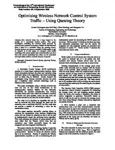
2.1. Local Monitoring Detection and Diagnosis Primitive Local monitoring is a collaborative detection strategy whereby each node in the network monitors the traffic of its neighbors. There is no separation of the WAHAS network into payload and monitoring systems, therefore, each node can potentially play a role in both systems. Local monitoring is the primitive that is used by all the protocols that we have developed to detect various control and data traffic attacks in WAHAS networks and diagnoses the malicious nodes involved in these attacks. Local monitoring requires that (i) each node in the network knows the identity of its first-hop neighbors and the neighbors of each neighbor, and (ii) each packet forwarder explicitly announces the immediate source of the packet it is forwarding. The first requirement holds by design of the routing protocol and the second requirement is satisfied through secure neighbor discovery protocols. The complexity of the secure neighbor discovery protocols vary between static and mobile WAHAS network and is thus one of the main challenges that we have addressed in this work, Chapter 4 and Chapter 7 respectively. For a node M to be able to monitor a node A over the link from X to A, M must be a neighbor of both A and X. In such a case, we call M a guard node of A over the link from X to A. In Figure 2.1, nodes M, N, and X are the guards of A over the link from X to A. For a link (i, j), the sender i is always a guard node for node j. Information for each packet sent from X to A is saved in a watch buffer at each guard for a time t. The information maintained depends on the particular attack under consideration. A malicious counter (MalC(i,j)) is maintained at each guard node, i, for every node, j, which i is monitoring over a sliding window of length Twin. The value of MalC(i,j) is incremented for any suspect malicious activity of j that is detected by i. The increment to MalC value
10
depends on the nature of the malicious activity, being higher for more severe infractions. To account for intermittent natural failures that can occur at legitimate nodes, a node is determined to be misbehaving, only if the MalC goes above a threshold (MalCth) over Twin. Examples of natural failures include collisions at the wireless media, environmental conditions, or passing barriers that may block or reduce the communication range. These natural failures may cause False alarms in which a “legitimate” node mistakenly consider another “legitimate” node to be malicious. A
X
M Y
B
X
A
D
The transmission range of node Y A guard node
N
Figure 2.1: X, M, and N are guards of A over link X to A In a general sense, the elementary activities underlying a large set of attacks in WAHAS networks are comprised of the following actions performed by the adversary node on an incoming packet–delay, drop, modify, misroute, and fabricate. There are elementary checking actions on the watch buffer for detecting each of these elementary malicious activities. The exact information stored in the watch buffer depends on the type of checking action–if delay, drop, misrouting, or fabrication is to be detected, then only the header information that uniquely identifies the packet (in my implementation, the sender and the sequence number) need be stored. If however, modification to the payload is also to be detected, then the payload body or a hash of it has also to be stored. The actions are specified in Table 2.1. These checking actions form the basis of my detection protocol. In this thesis, we discuss the detection for a representative set of attacks, though the elementary checking activities can be combined to detect a larger class of attacks. Table 2.1: Elementary malicious activity and checking action Elementary malicious activity Delay
Elementary checking action A packet lies unmatched in the buffer for time
11
Drop Modify
Fabricate Misrouting
greater than an application dependant threshold. Same as in delay. The outgoing packet does not match with the packet in the watch buffer. The matching may be either a bit-wise comparison of the unchanging fields in the packet (such as, the data, the original source and destination) or matching the hash values computed on these fields. The outgoing packet does not have a corresponding packet in the watch buffer. If the packet is forwarded to a next-hop node that is different from the one stored in the watch buffer.
Consider Figure 2.1 again, a node, say M, that can directly monitor the malicious behavior of its neighbor, say A, may be able to detect that neighbor. However, a node such as D that can not directly monitor the behavior of its neighbor, A, relies on alerts from other neighbors (M, X, N). When D gets enough alert messages about A, it believes in that A is malicious even though it has not directly noticed that. The notion of enough number of alerts is quantified by the detection confidence index (γ), Section 2.3. Each node maintains memory of nodes that it has revoked through a local blacklist so that a malicious node cannot come back to its neighborhood and claim to be blameless. Each entry in the blacklist consists of two fieldsthe identity of the malicious node and a onebit flag to indicate whether this malicious node has been detected directly or through the reception of g or more alerts from other nodes. 2.2. Local Monitoring Isolation Primitives A node is said to be integrated in the network if some of its first-hop neighbors accept its communication and is said to be revoked or isolated when all its first-hop neighbors reject its communication. Therefore, a revoked node can not receive any traffic from the network nor it can pass any traffic to the network. A node in the network only accepts traffic from or passes traffic to nodes that appear in its first-hop neighbor list. A node X revokes its neighbor node Y by deleting the entry of node Y in the first-hop neighbor list of X.
12
2.2.1. Local Response and Isolation When a node is determined to be malicious, it is important to take some action to neutralize the ability of the node to cause further damage. This is done by causing all the first-hop neighbors of the malicious node to revoke it. The local response and isolation primitive is used to propagate the detection knowledge to the first-hop neighbors of the malicious node and to take the appropriate response to isolate it from the network. Since detection knowledge propagates among neighbors of the malicious nodes, an authentication mechanism is assumed to exist in the network to prevent false accusation. The following local response algorithm is triggered by a guard node a when a node A is suspected because it’s malicious counter (MalC(α,A)) crosses the threshold, Ct. 1. Node a removes A from its neighbor list, and sends to each neighbor of A, say D, an authenticated alert message indicating that A is a suspected malicious node. The communication is authenticated using a shared symmetric key between a and D to prevent false accusations. Alternately, if the clocks of all the nodes in the network are loosely synchronized, a can do local two-hop authentic multicast as in TESLA [72],[73] or mTESLA [63] to inform the neighbors of A. Note the α isolates A without waiting for γ alerts from other nodes since a node definitely to trust itself. 2. When D receives the alert, it verifies its authenticity, that a is a neighbor to A, and that A is D’s neighbor. It then stores IDa in an alert buffer associated with A. 3. When D receives enough alerts, γ, about A, it isolates A by marking A’s status as void in the neighbor list. 4. After isolation, D does not accept any packet from or forward any packet to A. In addition to removing the malicious nodes from the network, this primitive makes the response process fast since the detection knowledge need not propagate throughout the network. This module is lightweight in the number of messages (one to
13
each neighbor of A, only on detection) and the number of hops each message traverses (maximum two hops). 2.2.2. Global Response and Isolation The process of local isolation described in the previous section is quick and lightweight, and has the desired effect of removing the potential for mischief of static malicious nodes. However, a mobile malicious node can move to a new location and perform some malicious activities before it is detected. Hence, the local isolation by itself is not enough to isolate mobile malicious nodes. In mobile scenarios a global mechanism is required to track and accumulate the malicious behavior of the mobile malicious nodes over all the locations it moves to. In such scenarios we introduced a central authority to track the malicious node’s behavior. The global response and isolation primitive is specific to mobile WAHAS network scenarios and is explained along with the protocols for mitigating attacks against mobile WAHAS networks, Chapter 7. 2.3. Selection of the Detection Confidence Index (γ) Value The detection confidence index is a design parameter in local monitoring used to enhance the capability of detection. However, γ introduces the possibility of framing among nodes. Framing is the process by which an innocent node is deliberately proved to be malicious by a quorum of malicious nodes. Therefore, the value of γ has to be chosen judiciously. The exact value of γ is application-specific and may range between one and infinity. A small value for g increases the chance of successful framing, while a large value of g increases the rate of harm a malicious node causes the network before being locally detected and isolated. If we set g to be infinity it means that a node only trusts itself in revoking a suspicious node, thus the local framing probability goes to zero. Any malicious node can be fully isolated as long as γ or more good guards detect it. However, if the number of good guards is less than γ, the node is only partially isolated from the network. Only the good guards that directly detect the malicious activity of the node isolate the malicious node. However, other neighbors of the malicious node continue to consider the malicious node as a legitimate node.
14
3. KEY MANAGEMENT: SECOS
Cryptographic keys are needed for secure communication between legitimate WAHAS nodes. The cryptography protocols for encryption and authentication use the keys. However, the security guarantees of any of these protocols are conditioned on the keys being available to all the legitimate nodes and no other nodes. The management of the keys (the process by which keys are generated, stored, protected, distributed, used, and destroyed) in a large-scale network of up to hundreds of thousands of sensor nodes is thus an important problem. Many WAHAS nodes are constrained in their energy availability, memory and computational resources, and communication bandwidth. These constraints make it impractical to use asymmetric algorithms for key management. These algorithms are computationally intensive, and consequently, energy intensive since at their heart they involve exponentiation and modulus operations of large numbers. The common approach, therefore, is to use symmetric key cryptography where the two endpoints of a communication share a secret key. The challenge is to manage the keys for symmetric cryptography in a scalable manner. The scalability goal implies that the endto-end communication delay, energy overhead for key management, and the dollar cost of deployment should increase gradually with increasing the size of the sensor network. Since WAHAS nodes may be placed in hostile environments, we must also design for the possibility that some nodes may be taken over or compromised. The WAHAS nodes are inherently less reliable than wired platforms and therefore, a protocol must be designed to function in the face of some nodes being unavailable. Radio communication is recognized as more energy consuming than computation by several orders of magnitude [41]. Consequently, the key management protocol should minimize the number of overhead control messages and the overhead number of bytes added to data messages.
15
Some symmetric key management protocols rely on a common shared secret key between all the nodes in the network leading to a highly insecure deployment. At the other end of the spectrum, some protocols have a separate shared key for each pair of nodes, which leads to a large amount of key storage that grows as the square of the number of nodes, and is therefore not scalable. The requirement to minimize communication overhead makes most of the proposed purely symmetric algorithms impractical for many WAHAS networks such as sensor networks since they add a fixed size overhead number of bytes to the payload and sensor networks typically have small sized packets. In this chapter, we propose and analyze a protocol called SECOS (Scalable & Energy-Efficient Secure Communication On Sensors) for key management in sensor networks that uses symmetric cryptography. The high-level design goals in SECOS are to (i) provide a scalable and secure key distribution channel for any-to-any communication in a large-scale sensor network, (ii) minimize the adverse fallout of compromising any sensor node, (iii) make key management energy efficient, and (iv) reduce the end-to-end delay of secure data communication. Using the well-known approach of node clustering [36]-[40], SECOS divides the sensor field into multiple control groups and assigns a rotating control node to each group. Communication within a group occurs through the use of keys exchanged with the help of the control node, while inter-group communication involves establishing a secure channel between the respective control nodes through the involvement of the base station. Effectively, SECOS imposes a three-level hierarchy of the nodes – a single base station, multiple control nodes, and a large number of sensing nodes. Of these, only the base station is fixed, assumed to be secure and assumed not to have any resource constraints, while all the rest, including the control nodes, are generic sensor nodes. Although node clustering is a well-known technique, it has to be used with special care for key distribution to protect the network against the compromised nodes that play a special role in node clustering. The control nodes are assumed to be susceptible to compromise and are monitored and can be removed from their privileged role. SECOS also provides techniques for secure initial deployment and revocation of suspect nodes.
16
A key decision choice in SECOS is the control group size. We present a simple mathematical analysis to determine an upper bound on the control group size, due to the resource constraints on the control node and the allowable security. We then present an equation that quantifies the energy cost of key management in terms of several factors, including the control group size, and derive the optimal control group size for the most energy-efficient key management. A promising approach for sensor key management has been proposed in a system called SPINS [63]. SPINS uses the base station as an intermediary for secure communication between any two nodes. We create a simulation model for comparing SECOS and SPINS with respect to end-to-end data latency and energy overhead of key management. For a fair comparison, we make the key caches also available to SPINS, though the original work does not mention caches. The simulation results show that SECOS reduces the energy consumption by a factor ranging from 1.2 to 7 and the end-toend data latency by a factor of 1.05 to 1.50 depending on the communication pattern and the cache size. A large cache means keys are available locally and then SECOS performs comparably to SPINS. However, this also implies additional storage requirement and the deployment is less secure to nodes being compromised. We provide a mathematical analysis to quantify the probability of exposing the communication between two legitimate nodes as a function of the number of compromised nodes. This is done for SECOS, SPINS [63], and a key pre-distribution protocol due to Du [64] and SECOS is shown to perform better for large operating regions. Many key management protocols for ad-hoc networks have been proposed in the literature. They suffer from one or more of the problems of weak security guarantees if some nodes are compromised, lack of scalability, high energy overhead for key management, and increased end-to-end data latency. In general, the key pre-distribution protocols [1],[9],[13]-[16],[63],[64], [18]-[20],[25] expose the security of the whole network when a certain fraction of nodes is compromised. Kerberos-like protocols (such as [62]) divide the network into several sections with privileged nodes for key management in each section. If the privileged node fails or is compromised, secure
17
communication in the entire section becomes impossible. A detailed comparison with existing schemes is presented in Section 8.1. The contributions of this work can be summarized as follow, 1. It provides a scalable protocol for key management that is sensitive to the sensor node’s resource constraints, including computation, communication, and bandwidth. We believe that current technology trends may remove some of the resource constraints, such as memory and processing power, in the foreseeable future, while the constraints of bandwidth and energy are expected to remain for some time to come. 2. It presents an energy efficient method for key management and substantial energy savings are demonstrated without introducing specialized high cost nodes in the network. 3. The protocol is resilient to some nodes being compromised due to attacks. In fact, it guarantees that, under a given set of assumptions, the communication between two uncompromised nodes cannot be exposed, irrespective of the number of other nodes that are compromised. Similarly, the protocol can tolerate some nodes being unavailable due to natural failures. SECOS uses several techniques well-known in the network security domain, such as node clustering, key refreshment, and neighborhood watch. Its contribution lies in synthesizing the different techniques into a cohesive protocol and applying that to the sensor network environment, with its distinctive constraints, chiefly, energy and susceptibility of the nodes to being physically compromised. We show that SECOS performs better with respect to existing state-of-the-art protocols for large parts of the normal operating region of sensor networks. In this paper, we do not describe the design in SECOS to address all forms of ID spoofing attacks and secure node addition to the existing network. The rest of this section is organized as follows. Section 3.1 presents the design of SECOS. Section 3.2 discusses how SECOS handles different classes of attacks. Section 3.3 presents a mathematical analysis for the maximum control group size and the energywise optimal control group size. Section 3.4 describes the message overhead in SECOS. Section 3.5 describes the experiments and the results.
18
3.1. Description of SECOS We use the following basic techniques in the design of SECOS. 1. Refreshing the keys and purging the caches. The keys are periodically refreshed and the key caches are purged regularly for two important security goals. The first is to minimize the adverse fallout of compromising some nodes in terms of the number of old messages that are exposed. The second goal is to defeat possible cryptanalysis attacks by analyzing plaintext and ciphertext pairs processed with the same encryption key. 2. Changing the nodes which play a privileged role. We do not wish to assume a large number of specialized well-protected nodes in our environment. Therefore, we design for the possibility of the nodes with special key management functionality being compromised and provide for them to be changed either on a time schedule, or when triggered by anomalous events. Another important goal of the control role rotation among the members of the control group is to achieve load balancing and even energy drain since the control node’s activities are more demanding. 3. Neighborhood watch. Each node maintains a list of its immediate neighbors and can overhear neighborhood traffic in order to detect compromised nodes. 3.1.1. System Assumptions and Attack Model Attack model: A malicious node can be either an external node that does not know the cryptographic keys, or an insider node, that possesses the keys. An insider node may be created, for example, by compromising a legitimate node. All these malicious nodes can exhibit Byzantine behavior and can collude amongst themselves. Any malicious node can for example eavesdrop on the traffic, inject new messages, replay and change old messages, spoof other identities, or pass traffic from one location of the network to a colluding node in another location (wormhole attack). System assumptions: SECOS assumes that the links are bi-directional, which means that if a node A can hear node B then B can hear A. Also, it assumes that the network has a static topology, though the functional roles a node plays (e.g., cluster head, data aggregator,
19
etc.) may change. SECOS also assumes that the sensor nodes are distributed uniformly on the sensor field. Moreover, it is assumed that the base station in SECOS is secure, not prone to failures, and does not have any resource constraints (bandwidth, energy, etc.). Protection against failures can be achieved by fault tolerant techniques such as redundancy for natural failures, or through a variety of possibly expensive security mechanisms, such as tamper proof hardware, for malicious failures. SECOS assumes that there is a certain amount of time from a node’s deployment, called the compromise threshold time (TComp) that is minimally required to compromise the node. We believe as in [20], [43], [44], that a sensor node deployed in a security critical environment must be designed to sustain possible break-in attacks at least for a short interval (say several seconds) when captured by the adversary; otherwise, the adversary could easily compromise all the nodes and thus take over the network. Therefore, instead of assuming that sensor nodes are tamper resistant which often turns out not to be true and very expensive, we assume there exists a lower bound on the time interval Tcomp that is necessary for an adversary to compromise a sensor node, and that the time TND for a newly deployed sensor node to discover its immediate neighbors is smaller than Tcomp. In practice, we expect TND to be of the order of several seconds, so we believe it is a reasonable assumption that Tcomp > TND. The current generation of sensor nodes can transmit at the rate of 40 Kbps [45] whereas the size of an ID announcement message is very small (12 bytes if an ID is 4 bytes and the hardware address size is 8 bytes).The probability of collision is quite small when a non-persistent CSMA protocol is used for medium access control [46]. Moreover, a node can broadcast its ID multiple times to increase the probability that it is received by all its neighbors. Furthermore, SECOS assumes that no external node exists in the network during the neighbor discovery. 3.1.2. Keys in SECOS SECOS uses five types of keys: the master key, the volatile secret key, the session key, the authentication key (MAC key), and the pseudo random number generator key (seed). The following notations for keys are used throughout this chapter. KAB (=KBA) refers to any secret key shared between A and B. The five kinds of keys – the master key,
20
the volatile secret key, the session key, the Authentication (MAC) key, and the random number generator key, will be denoted respectively as MKAB, VKAB, SKAB, AKAB, and RKAB Figure 3.1. E(K,X) denotes the encryption of a message X using key K. MAC(K,Z⊕X||Y) refers to the application of the MAC algorithm, keyed by key K, to the result of the concatenation of Y with the result of Z xor-ed with X. H(X) is the hash value of X. Any symmetric key encryption algorithm suitable for sensor networks may be used for encryption and decryption. It is desirable that the cipher text be the same length as the plaintext in order to reduce the message transmission overhead. An example of such a protocol is the counter mode (CTR) of block ciphers [12],[14]. Any underlying block cipher algorithm could be used with the CTR mode, e.g. DES [32] and its variants 3DES and DES-X, Rijindael [33], AES [33], TEA [34], and RC5 [35]. {MKMA, MKMB, MKMC}, {VKMA, VKMB, VKMC}
{JKMA, JKMB, JKMC}, J=M,S,A {H(VKMA), H(VKMB), H(VKMC)}
{CounterMA, CounterMB, CounterMC}
M
M A
B
C
MKAM
MKBM
MKCM
VKAM
VKBM
VKCM
CounterAM
CounterBM CounterCM
(a)
A MKAM SKAM AKAM RKAM H(VKAM)
B MKBM SKBM AKBM RKBM H(VKBM)
C MKCM SKCM AKCM RKCM H(VKCM)
(b)
Secure Session SKXY = MAC(MKXY,SC(X,Y)⊕ VKXY|| 1); AKXY = MAC(MKXY, SC(X,Y)⊕ VKXY|| 2); RKXY = MAC(MKXY,SC(X,Y)⊕ VKXY|| 3); New VKXY = H(VKXY), the hash value of VKXY.
Figure 3.1: Initial key setup between base station and three sensing nodes The master key is burnt into each sensor node at manufacture time and is shared with the base station. It is not used for encrypting message communication channels, but instead to generate other keys to be used for encryption and authentication. Compromising the communication channel does not reveal the master key since it is not used in any channel communication. The volatile secret key is also shared between the node and the base station. It is used, along with the master key, to generate the session and MAC keys. After each generation of session and MAC keys, a new volatile secret key is generated by applying a hash function to the current volatile secret key, after which the
21
current one is deleted and replaced by the new one. This provides SECOS with forward secrecy; if a node gets compromised, previous communications of the node are not exposed. This is due to the fact that the attacker is not able to generate the old keys since the earlier volatile secret keys are not available at the time of compromise, even though the master key is. As in the case of the master key, crypt-analyzing the communication does not reveal the volatile secret key since it is not used in any channel communication. The base station also shares two counters with each sensing node, one for each direction (sending and receiving) of communication SC(M,S) and RC(M,S). These counters are kept synchronized by incrementing them on messages sent or received between the sensor and the base station. During synchronization, the receive-counter value at one party is matched with the send-counter value at the other party. However, the counters need not to be exactly synchronized; they can be off by some known number Sync_diff. When the counters are not synchronized, the key generated at the base station using SC(M,S) may not match the one generated at the sensor node using RC(S,M). Therefore, the sensor node adjusts (increments/decrements) RC(S,M), generates the key, and compares the key with that generated by M. The sensor node continues to do that until the keys are either matched or the number of adjustments to RC(S,M) equals Sync_diff. In the latter case the sensor nodes initiate counter synchronization with the base station. In addition to the conventional use of counters to achieve semantic security, they are used in SECOS as a variable input for key generation. The semantic security prevents a malicious node from replaying old, properly authenticated messages that was used to establish keys between legitimate nodes. The use as the variable input is required in the key generation process to introduce randomness. These counters are used to replace the job of a nonce or a sequence number that ordinarily would be attached to every message to prevent the replay of old messages. However, due to the fact that communication is far more energy consuming than computation [49], we use the shared synchronized counters to minimize the transmission overhead of the sequence number or the nonce with every message. Figure 3.2 presents an algorithm that is used to synchronize the counters during key refreshment. Therefore, for most of the time, the counter synchronization does not incur any overhead and comes as a by-product of key
22
refreshment. For example during the course of our simulations no counter synchronization is required beyond that with the key refreshment. New keys are generated by applying MAC and hash functions over data that includes these counters. Figure 3.1 (a) shows the initial keying material that includes the master key, the volatile secret key, and the counters. The rest of the keys are derived from the previous two keys with the help of MAC (e.g. HMAC) and hash (e.g. SHA-1) functions that are preloaded on the base station and the sensors. The session key between the base station and a sensor node is generated by the base station, by applying a MAC function over the result of concatenating the binary representation of the number 1 with the result of the SC(M,S) XOR-ed with the volatile secret key. The same session key is generated by the sensor node by applying a MAC function over the result of concatenating the binary representation of the number 1 with the result of the RC(S,M) XOR-ed with the volatile secret key. The MAC function is keyed by the master key as shown in the bottom of Figure 3.1 for SKXY. The purpose of the session key is to provide data confidentiality for communication between two nodes. A similar mechanism is used to generate a shared authentication key between the base station and the sensing node with concatenation of the binary representation of the number 2 instead of the number 1, as shown in the bottom of Figure 3.1 for AKXY. SECOS uses independent keys for encryption and authentication since it prevents any potential interaction between the primitives that might introduce a weakness and is therefore a good security design principle. SECOS uses the standard key refreshment procedure for the session key and the authentication key. The session key and the authentication key are refreshed periodically or when triggered by a certain event, such as the detection of an attack. The pseudo random key is generated by each entity by applying a MAC function over the same parameters as for the session key with concatenation of the binary representation of the number 3. This key is used as a seed for the pseudo random number generator (e.g. RC4), which is used to produce the stream cipher such as in the CTR mode of DES [14]. This key is refreshed only when the pseudo random string it generates is exhausted, which depends on the pseudo random number generator algorithm used.
23 1.
M generates a new session key: SKMS = MAC(MKMS, SC(M,S) ∆ VKMS || 1).
2.
M generates a new Authentication key: AKMS = MAC(MKMS, SC(M,S) ∆ VKMS || 2).
3.
M Î S: CounterMS, Change, MAC (AKMS, CounterMS || Change).
4.
S generates a new session key: new (SKSM) = MAC(MKSM, RC(S,M) ∆ VKSM || 1).
5.
S generates a new Authentication key: new (AKSM) = MAC(MKSM, RC(S,M) ∆ VKSM || 2).
6.
S generates the next volatile secret key: VKSM = H(VKSM).
7.
S Î M: CounterSM, MAC(AKSM, CounterSM).
8.
M generates the new volatile secret key: new (VKMS) = H(VKMS).
9.
After the key refreshment is completed, all the old keys are purged.
1,2&9 M
7
3
S 4,5,6,8&9
Figure 3.2: Key refreshment and counter synchronization procedure Sometimes a packet sent from a source may not reach its final destination either due to a malicious event such as a compromised node in the path dropping the packet or due to natural node or link failure. As a result, the shared counters between these two parties may become unsynchronized, and a procedure has to be invoked to resynchronize them. Key refreshment is accompanied by shared counter synchronization between the two parties. However, the counter synchronization could be launched without the need to refresh any key. Figure 3.2 shows the key refreshment procedure between, the base station, M, and a regular sensor node, S. The one-bit flag, Change, is used if the counter synchronization is accompanied by key refreshment. 3.1.3. SECOS Structure A flat layout with a powerful base station and sensing nodes distributed through the sensor field and the base station being responsible for key management is clearly not scalable to a large number of nodes. This motivates the hierarchical structure of SECOS. The hierarchical structure we propose for SECOS has clusters of sensor nodes based on geographical proximity. Each cluster has a specially designated node called the Control Node, which plays a privileged role for key management. The cluster is called a Control Group. SECOS does not impose any special requirements on the control node, and it can be any ordinary sensor node in the cluster. This has the advantage of reducing the possibility of targeted DOS attacks to the specialized nodes. The control node acts as the intermediary for key management. It is periodically changed for the purpose of security
24
(the control node may get compromised), and for more even energy drain (the control node and its neighboring relay nodes drain energy faster). This hierarchical structure shown in Figure 3.3 consists of three levels of nodes. The root is the base station that is assumed to have powerful resources and is well protected. The internal nodes are regular sensor nodes selected to play the role of control nodes. The leaves are regular sensor nodes.
M Control Group
C1
S
...
C2
S
S
...
S
.
.
.
.
.
.
CB
S
...
S
S: Sensing Node Ci : Control Node M: Base Station
Figure 3.3: Three level hierarchy for key management in SECOS An important parameter in SECOS is the size of the control group. The size has two sets of determining factors, which exert opposing effects. The size has to be bounded within a maximum due to three factors―the resource constraints of the control node, such as the communication bandwidth and the computation capacity; the security concerns of not exposing too many nodes if the control node is compromised; and limiting the energy overhead of intra-group key management by bounding the distance between a sensor node and its control node. However, the size has to be kept above a threshold so that most communication occurs within a control group rather than involving multiple control groups since intra-group communication is more energy efficient than inter-group communication. Section 3.3 provides a detailed mathematical analysis of the control group size.
25
3.1.4. Topology Building and Maintenance It is necessary for the base station to have information about the topology of the network and for each node to have some local topology information. Here, we discuss how such information is initially obtained and subsequently how it is updated and maintained. As mentioned earlier in Section 3.1.2, each sensor shares a master key, a volatile secret key, and two counters with the base station from which each sensor node, upon deployment, computes shared session and MAC keys with the base station. As a result, a secure session is established between each node in the network and the base station. Also, in the initial deployment phase of the network, each node builds a list of its neighbors and communicates this list to the base station. SECOS assumes that a node cannot be compromised and no external malicious nodes exist within the time it takes to build this list, thus implying that the base station gets a correct view of the neighbor information. We say that two nodes, X and Y, are neighbors if X can hear the transmission of Y. Since SECOS only considers bi-directional links, this implies that Y can also hear the transmission of X. The list of neighbors at each sensor node is built by locally broadcasting a HELLO message, which is a small packet holding the ID of the sender, and then receiving a reply message, which is also a small packet holding the ID of the sender from each node that heard the HELLO message. As soon as the sensor nodes are spread in the sensor field, each node S broadcasts the HELLO message. For each reply received, S adds the sender ID to its neighbor list. Then S sends the full list to the base station authenticated using the authentication key shared between S and M (AKMS). Note that neighbor discovery is secure based on our assumption that no malicious nodes exist in the network during the neighbor discovery. Also note that neighbor discovery incurs a relatively negligible overhead since it is performed only once during the deployment of the network which is assumed to be static. This process is shown in Figure 3.4. The base station uses these lists to build a connectivity graph that represents the initial network topology and from that the control groups. The connectivity graph is built using an NµN connectivity matrix that is initialized to 0. For every member i in the neighbor list of S that M receives, M sets the entry (S,i) of the connectivity matrix to 1. The base station
26
generates the control groups using the connectivity matrix and the knowledge of the limits on the control group size and the maximum number of hops in the control group. For example, to generate the first control group, M adds node number 1 to the group, then the neighbors of node 1 are added, then the neighbors of each neighbor are added, and so on until the full control group is generated.
1.
S Æ one hop broadcast: HELLO.
2.
XÆ S: HELLO reply.
3.
S: adds the ID of X to its neighbor list (Snl).
4.
S: repeats 2 and 3 for every HELLO reply.
5.
S Æ M: MAC( AKSM, Snl || SC(S,M)).
M 5 1
1
A neighbor of S (e.g. X).
S 3&4
2
The communication range of S.
1 1
1 X
Figure 3.4 : Building the topology Alternately, a secure routing protocol such as INSENS [23] can be used to build the topology information and communicate it to the base station during the routing table construction. The base station has a global view of the entire network topology. When a compromised node is detected, its neighbors are informed, possibly through authenticated multicast [22]. 3.1.5. Assigning and Changing the Control Node The base station divides the network, based on the topology it built during the setup phase, into control groups consisting of geographically proximal nodes. For each control group, it then designates a node as a control node, say C, and sends it a list of session keys that the base station generates for each node in the group. The list of keys is sent in a message that is encrypted using the shared session key between the control node and the base station (SKMC). The session key is not sent to the sensing nodes in the group. Each sensing node generates that key on its own by applying a MAC function over the
27
result of concatenating the binary representation of 1 with the result of the RC(S,M) XOR-ed with the volatile secret key shared between the sensor node and the base station. The MAC function is keyed by the master key. This process is exactly identical to how the shared session key between the sensor node and the base station is generated independently by both parties as shown in the lower part of Figure 3.1 for SKXY. When a sensor node serves as a control node, it does not perform any sensing and uses all its available storage to store the keys. The motivation for this is to restrict the functionality of the control node to key management to facilitate control node monitoring by its neighbors. If the control node were to also send sensory data, it would be impossible for the neighbors to distinguish between control and data traffic since both are encrypted. Also, the key management functionality drains more energy than the regular sensing functionality and we wish to have as even a drain among the different nodes as possible. Finally, the control node requires memory resources to store the keys and does more computations to facilitate key management and we wish to reserve as much resource as possible for the control node to serve its control role. Typically sensor networks have redundant deployments whereby an event can be detected by multiple sensors. This leads us to believe that a reasonable number of nodes (the control nodes) may be exempted from the sensing functionality without adversely affecting the coverage on the sensor field. After the control node, C, receives the list of nodes in the control group, it broadcasts to the group members a message claiming that it is the new control node for the group. This message includes the list of neighbors of the control node that was built during the initial topology discovery phase. When a group member receives the claim, it buffers the claim. When the member needs to use C, it challenges C. The heart of the challenge lies in generating a random number using the random number generation key introduced earlier, authenticating it with the MAC key that should be available at the legitimate control node, asking C to do some processing on the number, and send it back authenticated. During this challenge the two nodes establish two shared counters between them. These two counters provide the same functionality as the SC(M,S) and RC(M,S) that are shared between each node and the base station. If the new control node
28
successfully passes the challenge, the sensor node replaces its current control node with the new one and if it is a neighbor node to the control node, it stores the list of neighbors of the new control node for the purpose of control node monitoring (Section 3.1.9). Note that now the node has a shared session key with the control node, which is different from the shared session key with the base station. The initial control node set up is shown in Figure 3.6. Figure 3.5 shows how a node, S, challenge a new control node, say C, in addition to the establishment of the shared counters between them. 5 1.
S hears the claim of C as a control node and buffers that claim.
2.
If S needs to use C, it generates two keys, SKSC and AKSC.
3.
S selects a random value using the pseudo-random number generator to be used as its SC(S,C).
4.
S Î C: SC(S,C), MAC(AKSC, SC(S,C)).
5.
C sets its RC(C,S) = SC(S,C).
6. 7.
C selects a random value using the pseudo-random number generator to be used as its SC(C,S). 2&3 C Î S: SC(C,S), MACKSC(3)(AKCS, SC(C,S) ∆ SC(S,C)).
8.
S sets its RC(S,C) = SC(C,S).
C
1
4
6
S
Broadcasting
Figure 3.5: Challenging the control node As mentioned in Section 3.1, we want to minimize the adverse fall out of a control node being compromised and provide tolerance against control node failures by regularly changing the control node. The control node is changed by the base station based on a certain time schedule, or when some anomalous events are detected, e.g., a compromised control node is detected. When the base station decides to initiate the change, it follows the same procedure as outlined above in this section for a new control node being assigned. In response to the announcement from the new control node, the previous control node, after challenging the new control node and being satisfied, flushes all the cryptographic data in its cache and returns to its normal sensing mode.
29
1- The base station, M, selects a new control node, C, for the control group, G.
M
2- M generates a new session key for each node, i, in G. SKiC = MAC(MAMi, SC(M,i) ⊕ VKMi || 1)
1&2 3 C 4
A
3- M sends to C a list of these generated session values MÆC: E(SKMC, {SKiC, IDi}), MAC(AKMC, E(SKMC, {SKiC, IDi}) || SC(M,C))
B
4- C announces its presence CÆ G members: I am a control node for group G
Figure 3.6: Control node refreshment 3.1.6. Key Caches Each sensor node has two types of caches: (i) Regular cache: stores the session keys used to encrypt data in message communication between itself and any other node. (ii) Key request cache: When a node initiates a data exchange and it does not have the session key for the receiver, it initiates a key establishment process. Subsequently, it may generate more data packets for the same receiver, before the key has been established. The key request cache stores the IDs of such receivers. In addition, a control node has two types of cache: (i) Ring cache: It stores the session keys between itself and each node in its control group. (ii) Control cache: It stores the session keys with other control nodes, which are used for inter-group communication. 3.1.7. Node to Node Communication within Control Group When a node, say A, needs to communicate with another node within its control group, say B, it first checks in its regular cache for the session key. If present, it uses the cached key. If not present, A generates two random keys K and K and encrypts one of them ( K ) using the other (K) as a key. Let us call K the Envelop. Node A sends the encrypted message E(K, K ) to B. Node A encrypts the key (K) and sends it to the control node C as E(SKAC,K). The control node recovers the key K, encrypts it E(SKBC,K), and forwards it to the destination B. When B receives the key K from the control node, it can
30
decrypt and obtain the key K that will be used as the shared session key between A and B. When B receives the message that A sent, it stores the message temporarily for the key to arrive from the control node. If B does not receive the key from the control node within a specified time, it drops the packet. Nodes A and B store the session key in their regular cache and continue to use it till the control node is changed, or the key is evicted due to cache replacement. The intra-group communication is shown schematically in Figure 3.7(a), and the detailed message communication is shown below: 1. A Î B: A, B, K( K ) 2. A Î C: A, B, E(SKAC,K), H(K), MAC(AKAC, A || B || E(SKAC,K) || H(K) ||SC(A,C)). 3. C Î A: A, B, E(SKBC,K), H(K), MAC(AKBC, A || B || E(SKBC,K) || H(K) || SC(C,B)) The MAC function is taken over the encrypted value of the Envelop. This has the advantage that the receiver doesn’t have to decrypt the Envelop if the MAC authentication fails, which saves some computation. 3.1.8. Node to Node Communication across Control Groups If node A wishes to communicate with a node that lies in a different control group, then two control nodes are involved. Say A lies in group G1 and B in G2 and the respective control nodes are C1 and C2. If A does not have the session key with B cached, A generates two random keys (K and K ) and sends the encrypted message E(K, K ) directly to B. Node A encrypts the key (K) and sends it to C1 as E(SKAC1, K). Node C1 checks its control cache for the session key between itself and C2. If not present, C1 generates a key, say U, and sends it encrypted to the base station as E(SKC1M, U). The base station forwards the key encrypted to C2 as E(SMC2, U). Notice that there is no need to send a direct packet from the source control node to the destination control node as in the communication between two nodes within a control group, since the base station is assumed to be trusted. After the session key between C1 and C2 is established (SKC1C2 = U), C1 sends the key K to C2 as E(SKC1C2, K), and C2 forwards the key to B as E(SKC2B,
31
K). Node B now has the key K and the message E(K, K ) from A and proceeds as in the intra-group communication to extract K and use it as the session key. (1) (2) (3) (4)
~
~
(1) E(K, K ); E(SKAC1, K), H(K) (2) E(SKC1M, U) (3) E(SKMC2, U) (4) Secure Session (C1,C2)
E(K, K) E(SKAC, K),H(K) E(SKCB, K),H(K) New secure session
M A 1
2
M C
4
3
B
(5) E(KC1C2, K), H(K) (6) E(K C2B, K), H(K) (7) Secure Session (A,B)
2 C1 1
3
4
C2 6
5 A
7 1
B
(b)
(a)
H(K):The hash value of K; SKxy: Session key between X & Y; M: Base Station; ~ A,B: Sensing Nodes; C: Control Node; (K,K ) : the Envelop and the key between A and B; U : the session key between C1 and C2. : A secure session
Figure 3.7: (a) Intra-group communication; (b) Inter-group communication using two control nodes. The two control nodes do not have a secure session when the process starts. The inter-group communication is shown schematically in Figure 3.7(b), and the detailed message exchange is shown in the following steps:
34-
A Æ B: A, B, E(K, K ) A Æ C1: A, B, E(SKAC1, K), H(K), MAC(AKAC1, A || B || E(SKAC1, K) || H(K) ||SC(A,C1)) C1 checks its control cache for C2, if an entry exists go to step 6 C1 Æ M: C1, C2, E(SKC1M, U), MAC(AKC1M, C1 || C2 || E(SKC1M, U) || SC(C1,M))
5-
M Æ C2: C1, C2, E(SMC2, U), MAC(AKMC2, C1 || C2 || E(SMC2, U) || SC(M,C2))
6-
C1 Æ C2: A, B, E(SKC1C2, K), H(K), MAC(AKC1C2, A || B || E(SKC1C2, K) || H(K) ||SC(C1,C2)) C2 Æ B : A, B, E(SKC2B, K), H(K), MAC(AKC2B, A || B || E(SKC2B, K)|| H(K) ||SC(C2,B))
12-
7-
32
3.1.9. Monitoring the Control Node The control node plays a privileged role in key management and a compromised control node can substantially affect the security of the network. Hence, it is important to monitor that the control node’s behavior does not deviate drastically from the expected functionality for key management. Occasional deviation is expected due to naturally occurring failures. Local monitoring, presented in Section 2.1, is used to detect any deviation in the functionality of the control node. If the control node is suspected as a malicious node, then the local response algorithm (Section 2.2.1) is called to propel the node from the network. However, it is more involved to detect if the control node C forwards a garbage packet instead of the Envelop. Since the communication from source A to C and C to the destination B are both encrypted, Figure 3.7 (a), local monitoring cannot observe the traffic. To solve the problem, A appends the hash of the Envelop to the packet. The hash is compared by C and if correct, re-appended to the packet before forwarding to B. Local monitoring can observe the hash values coming in and out of C and thus provide detection if the incoming and the outgoing hash values are different. If, however, the values are identical and B detects a mismatch, then C is considered suspicious by B that calls the local response algorithm (Section 02.2.1) to inform the neighbors of C about the detected suspicious activity. 3.2. Security Analysis In this section, we discuss the ability of SECOS to deal with the three major classes of security attacks–confidentiality violation, denial of service attacks, and authentication violation. 3.2.1. Confidentiality Attacks The key exchange protocol between two end points of a communication is described in Sections 3.1.7 and 3.1.8. We now show that this key exchange protocol does not reveal the shared key between two legitimate nodes irrespective of the number of compromised nodes if either of the following features is used. Note that these features are individually sufficient but not necessary for the proposition to hold.
33
1. The initial message E(K, K ) sent by the initiator of the key exchange, A, to the destination, B, cannot be obtained by the control node, or 2. The two parties involved in the key exchange, A and B, share an old session key in addition to K and use a combination of the new and previous session key for the communication. For example, if the previous session key was K , then A can use K ⊕ K
as the current session key for communication with B. In case a previous shared
session key is not available, nodes A and B must establish the session through the secure base station and not through the control node. Proposition: Under feature 1 or 2 above, it follows that compromising any number of nodes other than the two end-points does not reveal the shared key between them. This proposition holds even if the control node for the two end points is compromised. Proof: Case1: If feature number 1 is valid, then B is the only node in possession of the encrypted packet holding the key E(K, K ). Thus, the control node, C, does not have it and though it has K, it can never obtain the shared key K . Case2: If feature number 2 holds, the proposition can be proved using mathematical induction as follows. Base case: Let the number of compromised nodes in the network be NC. If NC = 0, there is no compromised node and the claim is trivially satisfied. If NC =1, this compromised node could be either the control node of A and B or any other node. If it is not the control node then the session can not be disclosed since only the control node, other than A, can decrypt the packet holding the Envelop. Consider that the single compromised node is the control node. Two cases are possible. (1) Nodes A and B have a previous shared key using an old control node. The current compromised control node does not know this key because the old control node was not compromised since the current control node is the only compromised node in the network by assumption. (2) Nodes A and B do not have a previous shared old key so they use the secure base station to start up the shared key and not the compromised control node. In both cases 1 and 2, the compromised control node cannot disclose the secure session between A and B.
34
Inductive step: Assume that the session between A and B is secure under (NC -1) compromised nodes, we want to show that it will be secure when a new node gets compromised for a total of NC compromised nodes. Inductive proof: If the NCth compromised node is not the control node, the claim is trivially satisfied. If the NCth node is the control node, then as in the base case, two cases are possible. (1) Nodes A and B share an old key (Kold), or (2) nodes A and B do not share an old key. In case (1), by the induction hypothesis, none of the (NC 1) compromised nodes know the key, Kold. The new compromised node does not know Kold since the key was exchanged before the node got compromised. So if the new key exchanged through the compromised control node is Knew , then the new session key will be (Kold ∆ Knew). While the compromised node can know Knew, it cannot know Kold. In case (2), nodes A and B do not share an old key and hence obtain their key directly from the secure base station. This exchange is done using the shared session key with the base station and therefore the key is unknown to the control node. This completes the proof of the proposition. Comments: The proof excludes the following cryptanalysis scenario. Assume the two nodes A and B have the startup key Kold from the main base station and then they use the Knew1 from control node C1, Knew2 from control node C2, …, Knewm from control node Cm. An attacker may capture the packet holding Kold and cryptanalyze it to obtain Kold. By the time this is done, the control node is Cm. Then the session key at that time will be Kold∆Knew1∆Knew2∆…∆Knewm. To know this key, the attacker must either compromise all the control nodes C1 up through Cm or crypt-analyze all the packets holding the keys Knew1 up through Knewm . It is expected that m will be a large number due to the small number of cipher packets the adversary has to crypt-analyze a key. It will be practically infeasible to compromise selectively all the control nodes C1, …, Cm, especially considering that control nodes are pseudo-randomly chosen from among the ordinary sensor nodes. Alternatively, it will be practically infeasible to crypt-analyze all the keys Knew1, …, Knewm.
35
However, it is possible, though difficult, that neither of the features mentioned above are satisfied. In feature 1, the control node may be able to buffer all packets between A and B, either directly or with the help of other malicious colluding nodes, and attempt to decrypt them and thus acquires K . Even if the communication of the initial message and the Envelop are randomized in time and order, it is possible that C buffers all messages within a window. Feature 2 is violated if the two parties do not share an old key and are unwilling to initiate key exchange using the main base station, possibly because it is far from either party. Section 3.2.1.1 presents a mathematical analysis of the probability of disclosing the secure session between A and B under certain number of compromised nodes if neither of the above features is used. 3.2.1.1. Probability of Secure Session Disclosure In this subsection we provide a mathematical analysis of the probability of compromising the link between two arbitrary nodes A and B lying in the same control group with the number of compromised nodes in the network being a parameter. For the purpose of comparison with other key management protocols, we assume in this analysis that only compromised nodes may exist in the network (no external malicious nodes). We perform the analysis for SECOS, SPINS (a representative Kerberos like protocol), and a protocol by Du et al. [64] (a representative key pre-distribution protocol), and compare the results. We assume that SPINS has as many base stations as the number of control groups in SECOS (NB) and that the nodes are uniformly distributed in the sensor field. For the mathematical analysis, we use a restricted version of SECOS which does not use the two features mentioned in Section 3.2.1, i.e., the node does not use the multiple keys from previous control nodes or the communication with the base station and the control node may overhear communication between the two nodes in its control group. This serves as a plausible operating region for the protocol where resources are constrained, the control group size is small, or the control node colludes with a neighbor of the source-destination pair. The restriction on SECOS also serves to shed light on the advantages obtained by a specific feature of SECOS, namely using two packets–K( K ) and the Envelop for key exchange between two arbitrary nodes. Note that if we use the
36
unrestricted version of SECOS, the analysis would become trivial since the probability of compromising the link between an uncompromised source-destination pair would be zero. To disclose the session key between A and B, an attacker must obtain both the Envelop (K) and the packet that is sent directly from A to B (E(K, K )). To obtain the Envelop, the control node for A and B must be compromised. To analyze the probability of capture of E(K, K ), we create a bounding path between A and B which is the rectangular bounding box containing nodes that may overhear the communication from A to B. This is shown by the dotted box in Figure 3.8. This is an overestimate since we use a square that circumscribes the circular transmission range of a node. To capture E(K, K
), there must be at least one node in the bounding path from A to B that is
compromised (we assume no compromised nodes exist in the network). Let the average number of hops between a pair of nodes in the control group be Hctrl, the density of nodes in the sensor field be D, and the communication range be R. The probability of capturing E(K, K )is less than or equal to the probability of having at least one compromised node in the bounding path. Let N be the total number of nodes in the sensor field and SGctrl=N/NB is the size of a control group. Let the number of compromised nodes in the network be NC and assume that the compromised nodes are uniformly distributed in the field. Let E2 represent the event that there is at least one compromised node in the bounding path. The identity of the current control node in a control group can be easily deduced by an attacker. However, as mentioned in the assumptions, it takes a finite amount of time Tcomp to compromise a node. The period of rotation of the control node is smaller than Tcomp. Thus, starting from an uncompromised network, it will be impossible for an attacker to compromise the control node after identifying it. So the attack model for the analysis is that the attacker randomly picks a node to compromise. Let E1 be the event that this randomly chosen node is a control node, for some arbitrary source-destination pair A and B.
37
2R
R
R
A
B
(H+1)R A sensor node
Communication range
A-B Bounding path
Figure 3.8: The bounding path between A and B The probability of E1 is
P ( E1 ) =
# Compromised Nodes N C = N #Nodes in Network
(3.1)
The probability of compromising the link between A and B (PA-B) is given by PA− B = P ( E1 E2 ) = P ( E2 | E1 ) P ( E1 )
(3.2)
The number of nodes within the bounding path Nbp is given by its area times the density of nodes in the network. N bp = ( H ctrl + 1) R ⋅ 2 R ⋅ D = 2( H ctrl + 1) R 2 D
(3.3)
Let E3 be the event that the control node exists in the bounding path. Then the probability of E3 is P ( E3 ) =
N bp SGctrl
(3.4)
Note that in the previous formula, we consider the size of the control group since A and B lie within the same control group.
P( E2 | E1 ) = P( E2 | E1 E3 ) P( E3 ) + P( E2 | E1 E3 ) P( E3 )
(3.5)
Let NG = N-NC represents the number of uncompromised (good) nodes in the network. The number of ways in which we can choose Nbp good nodes is NG − 2 N bp − 2
(3.6)
38
The total number of ways in which we can choose Nbp nodes is N −2 N bp − 2
(3.7)
Since A and B both are assumed to be non-compromised nodes, they are subtracted from Nbp, NG, and N. N G − 2 N bp − 2 P ( E2 | E1 E3 ) = 1 − N − 2 N bp − 2
PC ( A− B )
N G − 2 N − 2 N (1 − P ( E ) ) + 1.P( E ) = C 1 − bp 3 3 N − 2 N N 2 − bp
N − NC − 2 2 N C 2 R D ( H ctrl + 1) − 2 1 − P( E3 ) ) + P( E3 ) = ( 1 − N −2 N 2 2 R D ( H + 1) − 2 ctrl
(3.8)
(3.9)
In SPINS [63], which represents an example of the Kerberos-like protocols, the base stations are fixed. In order to make the sensor network economical, the authors assume that the base stations are not equipped with any specialized mechanisms or hardware to prevent compromise. They only assume that the base station has sufficient battery power to surpass the lifetime of all sensor nodes, sufficient memory to store cryptographic keys, and means for communicating with outside networks. Therefore the base stations in SPINS are equally likely to be compromised as any other sensor nodes. The model for the adversary is that it can target the base stations for compromising them. The attacker can identify the base stations and they are fixed so the adversary has enough time to try to compromise them. Thus, PC ( A− B )
NC if N C < N B = NB 1 if N ≥ N C B
(3.10)
39
The protocol by Du et al. [64] represents an example of a key-pre-distribution scheme and is summarized by us in Section 8.1. The authors present a corresponding calculation of PC(A-B) as PC ( A− B )
N τ τ = ∑ C 1 − i =δ +1 i ω ω NC
N C −i
(3.11)
Where d is the key space threshold, i.e. compromising (d+1) nodes will compromise the whole key space. w is the size of the key space’s pool, i.e. there are w key spaces for each node to pick from. t is the number of different key spaces that each node holds. The memory requirement at each node is mem = (d+1)µt . Also, they provide the formula for the probability that any two neighboring nodes can establish a secure session between them as Pactual
( (ω − τ )!) = 1−
2
SECOS
1.00 Probability of Link Disclosure
(3.12)
(ω − 2τ )!ω !
SPINS DU
0.80
0.60 0.40
0.20 0.00 30 80 130 180 230 280 330 380 430 480 530 580 630 680 730 780 830 880 930 Number of Compromised Nodes
Figure 3.9: Probability of compromising a randomly selected link between two uncompromised nodes as a function of the number of compromised nodes in the network.
Figure 3.9 shows the comparison among these three schemes (SECOS, SPINS, Du) using: w = 50, mem = 200, t=5, and Pactual=0.42 as parameters for Du’s scheme (d is
40
calculated as 39 based on the memory constraint mem), NB = 20 for SPINS, and. N = 2000, R = 30, D = 15 neighbors for each node, and Hctrl = 10 as parameters for SECOS. Notice that Du’s scheme has only 0.42 for Pactual while SECOS and SPINS both have 100% probability for any two nodes to establish a secure session between them. According to Figure 3.9, SECOS has lower probability of compromising a link than the other two protocols over a large range of the operating region. The probability goes to one for SPINS when the number of compromised nodes is greater than the number of base stations. Also, the link disclosure probability goes to one for Du’s scheme when the number of compromised nodes is greater than the d threshold. However, for a small number of compromised nodes, Du’s scheme is the most robust. 3.2.2. Denial of Service (DoS) Attack
1. DOS attack against a control node. This may be launched through a compromised node when it repeatedly asks the control node for forwarding a key. This kind of attack is handled by keeping a state vector at the control node for the currently active nodes that have recently requested key forwarding, and ignoring and sending feedback to the base station if a node behaves abnormally, e.g., asking for keys to communicate more than the feasible data rate. The feasible data rate is determined using a running window of the last m key requests and considers the communication bandwidth and the key cache size. 2. DOS attacks by a compromised control node: We reduce the probability of the presence of a compromised control node by a judicious selection of the control node based on trust level by periodically changing the control node. However, for the time period when a compromised node serves as a control node, it can prevent two legitimate nodes, A and B, from establishing a common key between them. In such a situation when the initiator cannot establish the secure session using the control node, it can perform the key exchange using the base station as an intermediary. Each of A and B share a session key with the base station, which is distinct from the shared session key with the control node, and this can be used to establish a secure channel. This solution is also valid when control node is unavailable due to a natural failure.
41
The base station verifies that the requests for Envelop forwarding are coming from a legitimate node in the network and if it finds the control node is non-existent, installs a new control node. This scheme is identical to that used in SPINS in the general noattack case. 3. DoS attacks against regular nodes: It is relevant to talk of only those DoS attacks against regular nodes that are enabled by mechanisms in SECOS. One possible DoS attack that may be launched against a legitimate node, B, is storage exhaustion by sending garbage packets to B, which buffers it in the expectation that the key needed to decrypt the packet is forthcoming from the control node. Requiring B to limit the number of unencrypted packets received from a specific source, accompanied by the inability of that source to launch an ID spoofing attack due to the neighbor watch (Section 3.2.3) alleviates this attack. 3.2.3. Authentication Attack
Another possible class of attacks is The ID spoofing and Sybil attacks in which a node impersonates other nodes [57] [76]. Through this attack, a compromised node can obtain knowledge of shared keys between other nodes. This class of attacks may be launched by a compromised control node, a regular node, or multiple nodes in collusion. SECOS handles the problem of regular nodes trying to masquerade as the control node by providing the control node challenge mechanism (Section 3.1.5) and for control nodes trying to masquerade as a different sensing node by using local monitoring (Section 3.1.9). The two kinds of authentication attack whereby a node impersonates a neighboring node or a non-neighboring node are detected by the neighbor watch mechanism by the neighbors of the compromised node according to the scheme described in Section 3.1.9. Note also that many key management protocols (e.g. [63],[9]) do not address the authentication problem. Key management protocols in [15] and [64] are examples which address authentication is an inherent property of their protocol. If the control node, C, is compromised, it may launch the following attack to uncover the key between two nodes in its control group, A and B. Node C sends to B a key K encrypted using the Envelop K claiming that it is from A. Node C performs the
42
same communication with A, claiming it is from B. Then C sends the Envelop K to both A and B after encrypting it with the respective session keys. The communication between A and B is now under the control of C. In SECOS, this attack is prevented through local monitoring in two different ways. First, if C tries to impersonate B and sends a packet, any of its neighbors, which does not have B in its neighbor list detects this while A itself will not be able to detect the impersonation. Second, if C generates the spurious messages and claims it is forwarding the message from B through a neighbor, say O, this is detected by the guard nodes for the communication through O, while it can not be detected by the destination, A. We quantify the overhead in terms of control messages for each of the operations in SECOS, such as key establishment within and across control groups, neighbor watch, and control node monitoring. 3.3. Determining Control Group Size
In this section, we perform mathematical analysis to determine the optimal control group size in SECOS based on the constraints of the sensor network and the desired level of security. We introduce some notations for this analysis. The regular cache size at each node is SC, the hit rate in the cache aC, and the miss rate bC =1-aC. The control cache size is SCC, and its hit and miss rates are aCC and bCC, respectively. The hit rate is the probability that an item is found in the cache while the miss rate is the probability that an item is missed from the cache. The control group size that is to be optimized is SGctrl, and the communication group size is SGcom. We introduce the communication group for a node as the neighborhood of that node, with which it predominantly communicates. The quantitative meaning of predominant is made clear in the particular discussion. For the analysis in this section, we assume that the communication happens completely within the communication group. Each node generates packets according to a Poisson process with rate 1/λ. The destination is chosen at random from the communication group. The destination is changed once every µ seconds on an average, again using an exponential distribution. The control node has an average lifetime of Tctrl. S(Pkt) gives the size of the
Pkt packet. Hcom, Hctrl, and Hall are the average number of hops between nodes within the same communication group, between a node and the control node, and between a node
43
and the base station. Energy gives the energy for transmission and reception of one bit. The summary and notations for some of the control packets used are given in Table 3.1. Table 3.1: Summary of relevant SECOS packet types Packet Notation
Description
K_req
The
Data
Envelop
from the
Packet Notation
Description
K_repf
Relay the Envelop from one
source to the control node
control node to another,
or from the control node to
used
the destination.
establishment
Data packet
K_rep
in inter-group key
The encrypted key from the source to the destination
3.3.1. Maximum Control Group Size
The maximum allowable size of the control group is determined by three factors– computational capabilities of the control node, bandwidth available around the control node, and the storage capacity for keys in the control node. These factors are discussed below. Here, GCOMP is the maximum control group size under the computational limitation only, GBW is the maximum control group size under the bandwidth limitation only, and GSTORE is the maximum control group size under the storage limitation only. 1. Computational Capabilities (GCOMP). The computational capability of the control node to service key requests from nodes in its group is one of the factors that bound the control group size. Assume that the computational capability of the control node allows it to process IP instructions per second and the encryption algorithm for the
Envelop encryption and decryption, the hash function computation, and the MAC encryption and decryption according to the steps shown in Figure 3.7(a) require IK instructions. The maximum number of keys that can be serviced is IP/IK keys per second. So if the node changes a destination every µ seconds and the miss rate in the regular cache is bC, a request is generated by a single node once every µ/bC seconds.
GCOPM ≤
IP ⋅ µ IK ⋅ β C
(3.13)
44
2. Channel Bandwidth (GBW). On average the available bandwidth for each node given channel bandwidth BW is BW/Nnbr where Nnbr is the number of one-hop neighbors of the node. Given the range of wireless transmission (r) and the density of nodes (ρ): D
= Л r2 ρ. Part of this traffic bandwidth is consumed by data. Thus the available BW for control communication (BWc) is the total bandwidth per node minus the amount of data traffic
BWc =
BW 2 S ( Data) − λ D
(3.14)
Each new session key served generates 2S(K_req) amount of traffic. Taking into account the regular cache misses and the key request rate this term is multiplied by (bC.1/µ). BWc ≥ GBW (2 ⋅ S ( K _ req))( β C / µ ) ⇒ GBW ≤ BWc /(2 ⋅ S ( K _ req )( β C / µ ))
(3.15)
Storage Capacity (GSTORE).The storage refers to the ring cache in the
3.
control node which stores the keys of nodes in the control group. If the storage requirement of each key is SKey and the available flash memory for the ring cache is FM, then the storage upper bound is given by GSTORE ≤ FM / S Key
(3.16)
The maximum size of the control group is the minimum of those calculated from equations (3.13),(3.15), and (3.16) above. Gmax = min(GCOMP , GBW , GSTORE )
(3.17)
The previous three factors came from resource constraints. A fourth factor arises from the security requirement. This is the security tolerance (GSEC) when a control node gets compromised. GSEC represents the maximum size of the control group under a certain acceptable number of compromised sessions or exposed messages. It is assumed that all the sessions that are established after the control node is compromised are disclosed. 4. Security tolerance (GSEC). We want to limit the amount of communication that will become exposed due to the control node being compromised. Let N(s) be the acceptable number of message communications that can be exposed. Let the rate at which nodes are compromised be λSEC. Consider a round as the time a control node
45
maintains its privileged position. The length of a round is Tctrl. Consider an infinitesimally small time slice dt, after time t has elapsed in a round. The number of nodes that can be compromised in this time slice is λSECdt. In the worst case, all the compromised nodes are control nodes. As a result of compromising these control nodes, the number of communication sessions that will become exposed are GSEC.((Tctrl-t)/µ)µbC. Integrating over the entire round, we have Tctrl
∫ 0
λSEC GSEC β C (Tctrl − t ) λ G β dt = SEC SEC C Tctrl 2 ≤ N ( S ) µ 2µ GSEC ≤
2µ N ( S ) λSEC βCTctrl 2
(3.18) (3.19)
The maximum size of the control group becomes, Gmax = min(GCOMP , GBW , GSTORE , GSEC )
(3.20)
3.3.2. Energy-Wise Optimal Control Group Size
Here we wish to find the optimal control group size based on security and energy concerns. For this analysis, we consider the energy consumed in the entire network per unit time, which is equivalent to the power requirement of the network. We want to increase the security by minimizing the time between control node refreshments and we want to decrease the overhead energy of the protocol. The security requirement favors decreasing the time to refresh the control nodes and the smallest is the best while a larger period is more optimal energy wise. So we shall proceed to optimize the energy overhead. In doing so, we face two conflicting factors. The first is the number of nodes that can be served by the same control node, and the second is the average number of hops to the control node. The first factor favors increasing the control group size, since that will reduce the occurrence of the energy expensive inter-control group key setup communication. The second factor favors decreasing the control group size, since that will reduce the number of hops between a sensing node and the control node. Three factors are to be considered for the overhead energy consumption of SECOS: the destination of the packet to be sent (whether within the same control group or
46
outside), the probability of regular cache hit, and the probability of control cache hit. In the following derivation, we assume that the average number of hops between nodes is proportional to the number of nodes under the same density and traffic conditions, such that: Hctrl = max (Hcomµ SGctrl /SGcom,,1). From these we derive the following four cases: Case 1: Hit in the regular cache. This occurs with probability aC that can be calculated as follows:
αC =
SC × λ λ SC N − 1 1 + 1 − ∑ SGcom × µ µ k =0 K N − 1
k
1 1 − N −1
N −1− k
(3.21)
The term (SCµl)/(SGcomµm) represents the probability that the key is found in the regular cache during the send of the first packet and the subsequent terms represent the probability that the second, the third, the fourth, etc packets hit. We assume that the size of the regular cache is greater than the number of packets sent in µ seconds. However, aC = 1 if the cache size is greater than the communication group size (SC > SGcom). If there is a hit in the regular cache, no overhead energy is spent. Weighted energy overhead = Energy overhead per miss. Probability = 0. Case 2: Miss in the regular cache and the destination is in the same control group. The probability of regular cache miss is bC = 1- aC. The probability of communication within one control group is SGctrl/SGcom. If SGctrl>SGcom, i.e., the control group is larger than the communication group, then the communication is always within one control group and the probability is one. Weighted energy overhead = Energy overhead per miss. Probability = SGctrl SGcom
( 2 × S (k _ req) + S (k _ rep) ) × H ctrl × Energy × βc ×
(3.22)
Case 3: Miss in the regular cache, the destination is outside the control group and hit in the control cache. The probability of control cache hit, given that the number of control groups within the communication group is NBC=SGcom/SGctrl, is given by:
aCC =
SCC/(N(SGcom)-1) = SCC/((SGcom/SGctrl)-1) = SGctrlµSCC/(SGcom-SGctrl). However, if SGctrl > SGcom/(SCC+1), aCC = 1. Weighted energy overhead =Energy overhead per miss. Probability =
47
{( 2 × S ( K _ req) + S ( K _ rep) ) H
ctrl
+ S ( K _ repf ) × H com } Energy
SGctrl SGctrl × SGcom ×β C 1 − SGcom SGcom − SGctrl
(3.23)
Case 4: Miss in the regular cache, the destination is outside the control group, and miss in the control cache .The probability of control cache miss bCC = 1 - aCC = 1 - SGctrlµSCC /(SGcom-SGctrl) = (SGcom-SGctrl-SGctrlµSGcom)/(SGcom-SGctrl) Weighted energy overhead = Energy overhead per miss. Probability
{( 2 × S ( K _ req) + S ( K _ rep) ) × H
ctrl
+ S (k _ repf ) × H com + 2 × S ( K _ req ) H all } Energy
SGctrl × SCC SGctrl × βC 1 − 1 − SGcom − SGctrl SGcom
(3.24)
The total overhead energy of the protocol equals the sum of the contributions of the above four cases. Let the size of the key reply be SR, i.e. S(K_rep)= SR. And since the size of key request equals the size of key reply forward which is approximately three times the size of the key reply, we have S(K_req) = S(K_repf) = 3SR. The total overhead energy TE is written as several separate equations each for a region bounded by discontinuities: If SGctrl > SGcom then TE = 7 × S R × H ctrl × Energy × β C
(3.25)
If SGctrl < SGcom and SGcom < SGctrl (SCC+1) then SGctrl TE = 7 × S R × H ctrl × Energy × βC SGcom SGctrl + (7 × S R × H ctrl + 3 × S R H com ) × Energy × βC 1 − SGcom If SGcom > SGctrl (SCC+1) then
(3.26)
48
SGctrl TE = 7 × S R × H ctrl × Energy × β C SGcom SGctrl SGctrl × SCC + (7 × S R × H ctrl + 3 × S R × H com ) × Energy × β C 1 − SGcom SGcom − SGctrl + ( 7 × S R × H ctrl + 3 × S R × H com + 6 × S R × H all ) Energy
(3.27)
SGctrl SGctrl × SCC ×β C 1 − SGcom SGcom − SGctrl We substitute Hctrl = 1 when SGctrl µHcom 1
δ
77
Figure 4.10: Sliding window illustration
The probability that G detects M during a certain time window (PgdM) equals the probability that M fabricates at least b packets within Twin, which is given by µ µ −i µ PgdM = ∑ (1 − Pfab ) Pfab i i=β i
(4.17)
The expected time of detection is calculated from the number of Twin time slots (Nts) that pass before the guard G detects the malicious node M. The probability that Nts = k is P ( N ts = k ) = PgdM (1 − PgdM )
k −1
(4.18)
Using Bernoulli trials, the expected value for Nts is given by E[Nts] =1/PgdM. The expected number of time slots (E[Nts]) before a single guard detects a malicious node is plotted in Figure 4.11. The plot shows that the latency decreases very fast with increasing probability of malicious behavior.
Figure 4.11: Expected number of time slots E[Nts] before a single guard detects a malicious node
For the case with overlapping sliding windows (η>1), Figure 4.10 (b), the analysis becomes more difficult and we use Martingale Theory [96] to obtain bounds on the delay. Here, we assume rate-based detection, i.e., a node is determined to be malicious if the rate of malicious activities goes above a threshold α. We present this
78
analysis for g = ∞ since it eliminates framing and is shown to give reasonable detection rates as shown through the simulations (Section 4.4). Let Xi be an i.i.d. Bernoulli random variable that tracks the number of malicious actions by a node, such that Xi=1 (malicious activity) with probability λ and zero, otherwise. Thus, E[Xi] = λ. Consider that the guard observes the node for Nact activities (packet forwarding actions). Define N act
Z N act = ∑ X i − N act λ
(4.19)
i =1
Then it can easily be shown that ZNact is a zero-mean martingale process. Similarly, YNact defined below is also a zero-mean martingale process N act
YN act = ∑ X i − ( N act − 1)λ
(4.20)
i=2
Now, let N0 be the number of activities at which the guard detects the node to be malicious. Then, N act
N 0 = min ∑ X i ≥ α N act N act
(4.21)
i =1
Our goal is to find E[N0]. From elementary probability, E[ N 0 ] = E[ N 0 | N 0 = 1] ⋅ P( N 0 = 1) + E[ N 0 | N 0 > 1] ⋅ P( N 0 > 1)
(4.22)
Note that E[N0|N0=1]P(N0=1) = 1×λ = λ. Also P(N0>1) = P(X1=0) = 1-λ. Next we find E[N0|N0>1]. Note that since YNact is a martingale, using the Optional Stopping Theorem [96], E[YN0] = E[Y2] = 0. Also, note that given N0>1, N act
N 0 = min ∑ X i ≥ α N act
(4.23)
N 0 = min YNact + ( N act − 1)λ ≥ α N act
(4.24)
N act
i=2
This means that given N0>1, N act
In other words, YN0 ≥ (α-λ)N0 + λ. Taking expectations on both sides, E[YN0 | N 0 > 1] ≥ (α − λ ) ⋅ E[ N 0 ] + λ ⇒ (α − λ ) ⋅ E[ N 0 ] + λ ≤ 0 ⇒ E[ N 0 | N 0 > 1] ≥ λ /(λ − α )
(4.25)
79
Therefore, de-conditioning, we get the lower bound as E[ N 0 ] ≥ λ + λ ⋅ (1 − λ ) /(λ − α )
(4.26)
For the upper bound we can repeat the arguments. Therefore, define Z N0 + λ ⋅ N 0 < α ⋅ N 0 + 1
(4.27)
The last term is because Xi≤1. Now, choosing α such that, λ < α (i.e., the rate of malicious activity is less than the detection threshold) and taking expectations we obtain 0 + E[ N 0 ] ⋅ (λ − α ) < 1 ⇒ E[ N 0 ] < 1/(λ − α )
(4.28)
Therefore, the bounds for the expected number of activities after which the guard will detect the node as malicious is,
λ ⋅ (1 − α ) /(λ − α ) < E[ N 0 ] < 1/(λ − α )
(4.29)
We plot Equation (4.29) in Figure 4.12 and find that the bounds asymptotically converge and exist only for λ > α.
Figure 4.12: Lower and upper bound for expected number of activities before a malicious node is detected by a guard 4.3.4. Cost Analysis
In this section, we show the memory, the computation, and the bandwidth overheads of LITEWORP to evaluate its suitability to resource-constrained environments.
80
4.3.4.1. Memory Overhead
We need to store the first and the second hop neighbor lists, the watch buffer, and the alert buffer. The identity of a node in the network is 4 bytes. Reusing the notation from the previous section, the size of neighbor list is NBL = pr2d entries. Each entry in the NBL needs 5 bytes; 4 for identity of the neighbor and 1 for the MalC associated with that neighbor. So the total NBL storage, NBLS=5(πr2d)2. For example, for an average of 10 neighbors per node, NBLS is less than half a kilobyte. The alert buffer has g number of 4 byte entries. The watch buffer size depends on the average number of hops between a source-destination pair, h, the frequency of route establishment, f, as well as the density of the nodes, d. To find the average number of nodes involved in watching a REP, we create a rectangular bounding box containing nodes that may overhear the REP sent from A to B (Figure 4.13). This is an overestimate since we use a square that circumscribes the circular transmission range. The number of nodes involved in monitoring is N REP = 2r 2 (h + 1)d
(4.30)
Thus, given N as the total number of nodes in the network, each node is involved in watching ( N REP / N ) f route replies per unit time. For example, if N=100 nodes, h = 4 hops, and f = 1 route every 4 time units, then NREP = 17, and each node watches only 4 route replies every 100 time units. Because the time t for which the packet is kept in the watch buffer is relatively small (may be less than one time unit), a watch buffer size of 4 entries is more than enough for this example. Each entry in the watch buffer is 20 bytes: 4 bytes each for the immediate source, the immediate destination, and the original source, and 8 bytes for the sequence number of the REP. If we include the route request in the watch, then each node will be involved in watching f + ( N REP / N ) f . That requires each node to watch 4 packets every 16 time units; again 4 entries are still sufficient for the watch buffer.
81
2r
r
A
r
B
(h+1)r A sensor node
Communication range
A-B Bounding path
Figure 4.13: The average number of nodes involved in the watch of a route reply 4.3.4.2. Computation and Bandwidth Overhead
Each watched route reply requires one lookup for the current source and the current destination in the neighbor list, adding an entry to the watch buffer (incoming) or deleting an entry from the watch buffer (outgoing), and may be another addition and deletion from the watch buffer (if a node is a guard for two consecutive links). Since the size of the watch buffer and the neighbor list structure are relatively small, the computation time required for these operations is negligible. For example, a lookup in a 100 entry buffer takes the MICA mote with an Atmega128 4-MHZ processor, about 2m seconds. The bandwidth overhead is incurred after deployment of a node for neighbor discovery and in the case of wormhole detection for informing the neighbors of the detected node. This is therefore a negligible fraction of the total bandwidth over the lifetime of the network. From the above analysis, we can conclude that LITEWORP has relatively modest memory, computation, and bandwidth overhead. This makes it especially suitable for resource-constrained sensor and ad-hoc networks. 4.4. Simulation Results
We use the ns-2 simulation environment [89] to simulate a data exchange protocol, individually in the baseline case without any protection, and with LITEWORP. We distribute the nodes randomly over a square field with a fixed average node density. Thus, the field size varies (80×80 m to 204×204 m) with the number of nodes. We use a
82
generic on-demand shortest path routing that floods route requests and unicasts route replies in the reverse direction. A route, once established, is not used forever but is evicted from the cache after a timeout period expires (TOutRoute). When a malicious node hears a route request, it directs the request to all the malicious nodes in the network using an out-of-band channel or using packet encapsulation. For packet encapsulation, we assume that the colluding nodes always have a route between them. We simulate the outof-band channel by letting the compromised nodes deliver the packets instantaneously to their colluding parties. These two schemes exercise the principal feature of LITEWORP, namely, local monitoring and are the most challenging to mitigate. Hence, we simulate them in preference to other modes of attack. After a wormhole is established, the malicious nodes at each end of the wormhole drop all the packets forwarded to them. Furthermore, a malicious node always frames its good neighbors. The simulation also accounts for losses due to natural collisions. The guards inform all the neighbors of the detected malicious node through multiple unicasts. For each run, malicious nodes are chosen at random such that they are more than 2 hops away from each other. Input parameter: Each node acts as a data source and generates data using an
exponential random distribution with inter-arrival rate of φ. The destination is chosen at random and is changed using an exponential random distribution with rate x. We use M for the number of malicious nodes, γ for the detection confidence, and N for the total number of nodes. The input parameters with the experimental values are given in Table 4.2. A design parameter in LITEWORP is the increment to the malicious counter value upon detecting a malicious event. On the one hand, we want the increment to be large for higher detection probability, fast detection, and small watch buffer size. On the other hand, we want the increment to be small to reduce the percentage of false alarms. We conduct an experiment to design the malicious counter increment. We choose the increment as the lower of the two points–the point where the percentage detection reaches its maxima and the point where the knee of the false detection curve lies. This gives us a reasonable combination of low false alarm rate and high detection rate. The value of the MalC increment used for the experiments is given in Table 4.2.
83
Output parameters: The output parameters include (i) the isolation latency which is
defined as the time between when the node performs its first malicious action to the time by which all the neighbors of the node have isolated it, (ii) the fraction of data packets dropped due to the wormhole to the data packet sent, (iii) the fraction of malicious routes to the total number of routes established. This parameter quantifies the amount of harm caused by the malicious nodes,, (iv) the percentage of framing, which is defined as the percentage of the number of good nodes that could be framed to the total number of nodes, (v) the percentage of false isolation, which is defined as the percentage of the number of nodes that have been isolated due to natural causes to the total number of nodes, and the percentage of malicious node isolation, which is defined as the number of malicious nodes isolated to the total number of malicious nodes. All the output parameters that we present here are measured at the end of the simulation time (1500 seconds) unless otherwise stated. The output parameters are obtained by averaging over 30 runs. Finally, the figures we present are for the 100-node scenario unless otherwise stated. Table 4.2: Input parameter values for LITEWORP simulations Parameter Tx Range (r) MalC incr. TOutRoute Ct
Value 30 m 10 50 sec 150
Parameter g φ M t
Value 3,5,7, infinity 0.2 sec 0-6 0.5 sec
Parameter # nodes (N) x BW Twin
Value 20,50,100,150 0.02 sec 40 kbps 200
Data packet drop: Figure 4.14 shows the number of packets dropped as a function of the
simulation time for 2 and 4 colluding nodes both with LITEWORP and without LITEWORP. The attack is started 50 sec after the start of the simulation. Since the numbers are vastly different in the two cases, they are shown on separate Y-axes; the axis on the left corresponds to the baseline case and the axis to the right corresponds to the system using LITEWORP. In the baseline case, since wormholes are not detected and isolated, the cumulative number of packets dropped continues to increase steadily with time. But in the LITEWORP case, as wormholes are identified and isolated permanently, the cumulative number stabilizes. Notice that the cumulative number of packets dropped
84
grows for some time even after the wormhole is locally isolated, due to the cached routes
3500
4 w/o LiteWorp 2 w/o LiteWorp 4 w/ LiteWorp 2 w/ LiteWorp
w/o LiteWorp
3000 2500 2000 1500 1000 500 0 0
50
100
200
300
400
500
160 140 120 100 80 60 40 20 0 600
With LiteWorp
that contain the wormhole and continue to be used till route timeout occurs.
Simulation time
Figure 4.14: Cumulative number of dropped packets with and without LITEWORP
Figure 4.15 shows a snapshot, at the end of the simulation time, of the fraction of data packets dropped and the fraction of malicious routes. This is shown for 0-4 compromised nodes for the baseline and with LITEWORP. With 0 or 1 compromised node, there is no adverse effect on normal traffic since no wormhole is created. The relationship between the number of dropped packets and the number of malicious routes is not linear. This is because the route established through the wormhole is more heavily used by data sources due to the aggressive nature of the malicious nodes at the ends of the wormhole. If we track these output parameters over time, with LITEWORP, they would tend to zero as no more malicious routes are established or packets dropped, while without LITEWORP they would reach a steady state as a fixed percentage of traffic continues to be affected by the undetected wormholes.
85
0.0120
fr. drop fr. mal routes fr. drop-LiteWorp fr. mal route-LiteWorp
0.60
0.0100 0.0080
0.40
0.0060 0.0040
0.20
0.0020
0.00
With LiteWorp
w/o LiteWorp
0.80
0.0000 0
1
2 3 #of malicious nodes
4
Figure 4.15: Fraction of dropped packets and malicious routes with and without LITEWORP
Figure 4.16 bears out the analytical result for the detection probability as γ is varied with NB = 15 and M= 2. As γ increases, the detection probability goes down due to the need for alarm reporting by a larger number of guards, in the presence of collisions. Also the isolation latency goes up, though it is very small (less than 30 s) even at the right end of the plot. 50-node scenario
30
P(Detection)
1
24
0.8
Sim P(detection) Ana P(detection) sim isolation latency
0.6
18 12
0.4 0.2
6
0
0 1
2
3
4
5
6
7
Isolation latency
1.2
8
Detection confidence index
Figure 4.16: Detection probability and latency with varying g Framing: Figure 4.17 shows the percentage of framing with various values of g. As the
number of malicious nodes increases, the chances of getting g malicious nodes framing a good node increases and thus the framing percentage increases. As we increase g, the percentage of framing decreases since it becomes more difficult to get g malicious nodes
86
to frame a good node. When the value of g is greater or equal to 7, the probability of framing goes to zero since no node has more than 7 neighbors in this simulation setup, therefore, it is impossible for framing to occur.
% Framed_nodes
35
GAMMA=1 GAMMA=3 GAMMA=7
28 21 14 7 0 2
6
10 14 18 22 Number of malicious nodes
26
30
Figure 4.17: Percentage of framing Varying the number of malicious nodes: Figure 4.18 shows the percentage of malicious
nodes isolated at the end of the simulation time for three different values of g. The isolation percentage falls almost linearly as we increase the number of colluding malicious nodes from 2 to 6 due to the decrease in the number of available guards. Note that as g increases, the percentage of malicious nodes isolated decreases slightly due the requirement of higher number of guards to agree on the detection. However, the % malicious nodes isolated is above 90% for 6 malicious nodes with infinite g. % Mal. Node Isolation
100 96 92
GAMMA=3 GAMMA=1 GAMMA=7
88 84 80 2
3
4 #Mal_nodes
5
Figure 4.18: Percentage of malicious node isolation
6
87
Figure 4.19 shows that the percentage of false isolation increases as the number of malicious nodes increases. This is because not all guard nodes come to the decision to isolate a malicious node at the same time. Therefore, a given guard node may suspect another guard node when the latter isolates a malicious node but the former still has not. For example, a guard node G1 detects a malicious node M earlier than the other guard nodes for the link to M. Node G1 subsequently drops all the traffic forwarded to M and is therefore suspected by other guard nodes for M. This problem can be solved by having an authenticated one-hop broadcast whenever a guard node performs a local isolation.
% False_Isolation
2
GAMMA=3 GAMMA=Infinity
1.6 1.2 0.8 0.4 0 2
3
4 #Mal_nodes
5
6
Figure 4.19: Percentage of false isolation
Figure 4.20 shows that the percentage of malicious routes increases as we increase the number of malicious nodes. As the number of malicious nodes increases, the percentage of damage that occurs before each of the nodes is detected and isolated increases.
% Mal_routes
1.5
GAMMA=3 GAMMA=Infinity
1.2 0.9 0.6 0.3 0 2
3
4 #Mal_nodes
5
Figure 4.20: Percentage of malicious routes
6
88
Varying g:: Figure 4.21 shows the percentage of false isolation as a function of g. As g
increases the false isolation decreases since it becomes more and more unlikely to get g nodes falsely accuse a good node as malicious. As the number of malicious nodes increases the false isolation increases for the same reasoning as in Figure 4.17.
% False_Isolation
6
Mal_nodes=6 Mal_nodes=2
4.8 3.6 2.4 1.2 0 1
3 5 7 Detection Confidence (GAMMA)
Infinity
Figure 4.21: Percentage of false isolation
Figure 4.22 shows that the percentage of malicious routes increases with g. As g increases, the detection and isolation of nodes decreases and takes longer time which gives the malicious nodes more chance to establish more malicious routes. Moreover, as the number of malicious nodes increases, the percentage of damage (malicious routes) increases intuitively.
% Mal_routes
1.6
Mal_nodes=6 Mal_nodes=2
1.3 1 0.7 0.4 0.1 1
3 5 7 Detection Confidence (GAMMA)
Infinity
Figure 4.22: Percentage of malicious routes
89
The observation from all the experiments is that an infinite value of γ appears to be a desirable operating region. We find that it eliminates framing and minimizes the percentage of false isolation. On the other hand, it only slightly increases the percentage of malicious routes and slightly decreases the percentage of malicious nodes isolated. However, these values are acceptable and close to the case when g is small. This is because the guards of a node over a certain link are likely to see the same view of the node and therefore, they are likely to reach to the same reasoning about the monitored node whether individually or through the reports of other guards. This reduces the importance of having guards inform each other of their view about the monitored node which results in little change when we increase the value of g to infinity.
90
5. MITIGATING OTHER CONTROL AND DATA TRAFFIC ATTACKS IN STATIC WAHAS NETWORKS: DICAS
The traffic in WAHAS networks can be broadly classified into data and control traffic. Control traffic contains information needed to set up the network for data traffic to flow. Typical examples of control traffic include routing, monitoring the liveness of nodes, topology discovery, and system management. Examples of data traffic include sensor readings and alert messages in surveillance environments. As mentioned earlier in the introduction (Chapter 1), the wireless media makes the traffic of WAHAS networks more susceptible to various kinds of attacks against both control and data traffic. Control traffic attacks include the (Ci) wormhole attack ([51],[53]), (Cii) the rushing attack [52], (Ciii) the Sybil attack [57], (Civ) the sinkhole attack [76], and (Cv) the HELLO flood attack [76]. Therefore, the wormhole attack presented in the previous chapter (Chapter 4) is one of many control traffic attacks against WAHAS networks. Control attacks are especially dangerous because they can be used to subvert the functionality of the routing protocol and create opportunities for a malicious node to launch data traffic attacks such as dropping all or a selective subset of data packets. In addition to control traffic attacks, WAHAS networks are also vulnerable to data traffic attacks. The most notable data traffic attacks are (Di) blackhole, (Dii) selective forwarding, (Diii) artificially delaying of packets, in which respectively a malicious node drops data (entirely or selectively) passing through it, or delays its forwarding, and (Div) misrouting attack in which the attacker relays packets to the wrong next-hop in an intention to indirectly drop them. The attacks could result in a significant loss of data or degradation of service.
91
These control and data traffic attacks affect many WAHAS network protocols presented in the literature. Table 5.1 enumerates some of theses protocols and their respective vulnerabilities summarized from the work presented by Karlof et al. [76]. Table 5.1: Examples of vulnerable WAHAS network protocols to control and data traffic attacks Routing protocol name Directional diffusion ([80], [81]) GPSR [99] Minimum cost forwarding [82] LEACH [58], PEGASIS [103] Rumor routing [83] SPAN [101]
Attacks Ciii, Civ, Cv, Dii Ciii, Dii Ci, Civ, Cv, Dii Cv, Dii Ci, Ciii, Civ, Dii Ciii, Cv
In this chapter, we extend the work presented in the previous chapter (Chapter 4) through providing new mitigation techniques for additional control and data traffic attacks in static WAHAS networks. We present a lightweight framework called DICAS (Detection, Diagnosis, and Isolation of Control and Data Attacks in Sensor Networks), which mitigates many control and data traffic attacks in static WAHAS networks. Again, DICAS not only detects the occurrence of an attack, but also diagnoses the malicious nodes involved in it and removes their capability of launching future attacks by isolating them from the network. The detection and isolation mechanisms are executed locally, without incurring a significant overhead. DICAS is especially suited to the low cost point of sensor networks since it does not require any specialized hardware (such as directional antennas [1] or GPS) nor does it require time-synchronization among the nodes [53]. DICAS achieves its security goals by exploiting local monitoring (Section 2.1). We systematically lay out the fundamental structures and the state to be maintained at each node for mitigating some representative attacks – Sybil, wormhole, rushing, selective forwarding, and misrouting attacks. The first three are examples of attacks directed to control traffic while the last two are examples of attacks directed at data traffic. Independent of the detection mechanism, we use local isolation (Section 2.2.1) to isolate malicious nodes locally in a distributed manner.
92
In this chapter we consider the possibility of monitoring the data traffic in addition to the control traffic to mitigate various control and data traffic attack. This is in contrast to the previous chapter in which guards monitor only the control traffic. This enables us to detect and isolate the attacker at any point during the network activity, even if we fail to do so using the control traffic or the adversary stays benign during exchange of control traffic. It is important to be able to use the data traffic in detection and isolation of attackers since in some network scenarios, the frequency of control traffic exchange may not be sufficient to detect malicious nodes if the protocol wants to maintain a low incidence of false detection. However, monitoring data traffic is not trivial because of the vastly increased volume compared to control traffic. Hence, we investigate the effect of partial sampling of data traffic on the metrics of detection and isolation. We use DICAS to create a novel lightweight secure routing protocol called LSR that withstands known attacks against the routing infrastructure and provides additional protection against data attacks by supporting secure node-disjoint multiple route discovery. We analyze the detection coverage and the probability of false detection of DICAS. We also evaluate the memory, communication, and computation overhead of DICAS. Finally, we simulate the wormhole attack in ns-2 and show its effect on the network performance with and without DICAS. The results show that DICAS can achieve 100% detection of the wormholes for a wide range of network densities. They also show that the detection and isolation of the nodes involved in the wormhole can be achieved in a fairly short time after an attack starts. In addition, we simulate a combined Sybil and rushing attack to bring out the adverse impact on node-disjoint multipath routing and show the improvement using DICAS. The results show that LSR using DICAS is resilient to the combined attack and that the average number of node-disjoint routes discovered is not reduced. Our experiments with data monitoring show the feasibility of detecting the selective forwarding attack while monitoring only a fraction of the data traffic. In summary, the contributions in this chapter include, •
Proposing a mechanism to detect any control or data attack that directly manifests
itself in one of dropping, delaying, modifying, misrouting, or fabricating of packets.
93
•
Developing a toolset based on overheard information that can be mapped to detecting
different classes of attacks. We analyze this toolset for different metrics, such as, false alarm probability, missed alarm probability, and latency of isolation. •
Proposing a mechanism that, based on information collected by the toolset, allows for
diagnosing and isolating the malicious nodes. •
Demonstrating the effectiveness of the toolset applied to both data and control attacks
through simulations. The rest of this chapter is organized as follows. Sections 5.1 describes DICAS. Section 5.2 describes LSR. Section 5.3 presents representative examples of control and data attacks and their mitigation using LSR with DICAS. Section 5.4 analyzes the coverage and overhead of DICAS, while Section 5.5 presents simulation results. 5.1. Description of DICAS
In its goal of providing detection and isolation to control and data attacks, DICAS provides the following primitives - neighbor discovery and one-hop source authentication (Section 5.1.2). These two primitives are used with local monitoring (Section 2.1) and local response (Section 2.2.1) to provide mitigation for various attacks. 5.1.1. System Model and Assumptions Attacker model: This model is the same as that of LITEWORP (Section 4.2.1), however
we repeat it here for convenience. An attacker can control an external node (i.e., a node that does not know the cryptographic keys that allows it to be authenticated by the rest of the nodes), or an internal node, (i.e., a node that possesses all the keys required for it to be authenticated by other nodes in the network, but exhibits malicious behavior). An insider node may be created, for example, by compromising a legitimate node. A malicious node can perform all the attacks mentioned in the introduction of this chapter, by itself or by colluding with other nodes. A malicious node can establish out-of-band fast channels (e.g., a wired link) or have a high powered transmission capability.
94
System assumptions: These assumptions the same as those of LITEWORP (Section 4.2.1),
however, we repeat them here for convenience. DICAS assumes that all the communication links are bi-directional. A finite amount of time is required from a node’s deployment for it to be compromised, and to perform the first- and second-hop neighbor discovery protocol. We assume that no external or internal malicious nodes exist before the completion of the neighbor discovery. However, we can remove this assumption and use one of the protocols for secure neighbor discovery such as the directional antenna by Hu and Evans [51]at the additional cost of using directional antennas or by using trusted and more powerful nodes as in [95]. DICAS assumes that the network has sufficient redundancy, such that each node has more than an application defined threshold number of legitimate nodes as guards. DICAS assumes that the network has a static topology. This does not rule out route changes due to natural and malicious node failures or route evictions from the routing cache. Moreover, DICAS assumes that each packet forwarder explicitly announces the immediate source of the packet it is forwarding. Finally, DICAS assumes a key management protocol, e.g., [64], is used to pre-distribute pair-wise keys such that any two nodes in the network can securely communicate with each other. 5.1.2. Primitives: Neighbor Discovery and One Hop Source Authentication Neighbor discovery: This protocol is used to build a data structure of the first hop
neighbors of each node and the neighbors of each neighbor. The data structure is used in local monitoring to detect malicious nodes and in local response to isolate these nodes. A neighbor of a node, W, is any node that lies within the transmission range of W. As soon as a node, say A, is deployed in the field, it sends a one-hop broadcast of a HELLO message. Any node that receives the message sends a reply back to A. For each reply received within a pre-defined timeout (TROUT,), A adds the responder to its neighbor list, RA. Let RA = W1, ..., Wp and Msg = RA||Kcommit(A), where Kcommit(A) is the commitment key A uses later to authenticate itself to its neighbors. Node A then sends a one-hop broadcast of Msg. A node Wj that receives Msg, stores RA (Wj’s second-hop neighbors) and Kcommit(A). Hence, at the end of this neighbor discovery process, each node has a list of its direct neighbors and their neighbors as well as the commitment key of each one of its direct
95
neighbors. This process is performed only once in the lifetime of a node and is secure in static wireless networks that follow our assumptions of attack-free environment during neighbor discovery. Commitment key generation and update: This protocol is used to generate and update
the commitment key used by the one-hop source authentication protocol. The values of the commitment key at a node S (Kcommit(S)) are derived from a random seed (Kseed(S)) as Kcommit(S) = H(i) (Kseed(S)), where H is a one-way collision resistant hash function [112][114], i takes values between 0 and l(¥2), and l is the length of the sequence of values of Kcommit(S) that we call the commitment string. The first value of the commitment key Kcommit(S) that is exchanged with the neighbors during neighbor discovery is H(l)(Kseed(S)) = vl. The subsequent values of the commitment key (vl-1,…, v0) are progressively disclosed to the neighbors during subsequent transmissions. Before the current commitment string {vl, vl-1,…, v0} is exhausted, a new one is generated at S {ul, ul-1,…,u0}. The commitment key ul from the new string is authenticated to the neighbors using the last undisclosed key from the current string with the one-hop source authentication protocol. One-hop source authentication: This protocol allows a node to distinguish between its
neighbors to prevent identity spoofing among them. A node S authenticates its transmitted packets to the neighbors by attaching the last undisclosed value from the commitment string Kcommit(S). This authentication is only used with the source of the packet, not at every hop in the path of the packet from the source to the destination . When a neighbor of S, say B, receives the packet, it verifies the validity of Kcommit(S) by computing a hash function over it and comparing the result with the stored value of Kcommit(S). If Kcommit(S)
is valid, B stores it as the new commitment key value of S.
However, this protocol may fail to provide the required authentication if an attacker blocks the transmission range of a certain source from the rest of network except itself. Therefore, the attacker can impersonate that source and generate valid packets. In such case, we revert to the well-known mTESLA authentication scheme [62][63] which countermeasures such attacks.
96
5.1.3. Application of Local Monitoring for Data Attacks
Chapter 4 presents the application of local monitoring to the wormhole attack through monitoring the control traffic. Moreover, Chapter 2 presents the elementary activities underlying a large set of attacks in an ad-hoc multi-hop network. These activities are comprised of the following actions performed by the adversary node on an incoming packet – delay, drop, modify, and fabricate. Also, Chapter 2 presents the exact information stored in the watch buffer for each malicious action and the corresponding checking details of each. This section expands the attack-set mitigated by local monitoring to include data attacks. DICAS refers to data attacks as the general class of attacks directed at the data traffic after the route has been established. The objective of these attacks is to disrupt the end-to-end transmission of data between a source and a destination. The disruption can be done through leaking information or through launching denial of service by manipulating the data. When leaking information, the adversary node does not manipulate the data but gathers information based on data that flows through it. In the denial of service attack, the adversary actively manipulates the data packets through delay, drop, fabrication, or modification. Information leaking is difficult to detect by monitoring the data traffic alone. This mode of attack becomes particularly insidious when the adversary uses control attacks such as the wormhole attack to create an opportunity to control a disproportionately large portion of the routes in the network. We use the local monitoring approach applied to the control traffic to mitigate this mode of attack. For the second class of data attacks (DoS by manipulating the data), local monitoring can be applied to the data traffic using the elementary checking activities mentioned in Table 2.1. This approach is useful in particular where an adversary node is in the position of having large amounts of data traffic flowing through it due to its strategic position in the network, without the need to launch a wormhole attack. The detection of data traffic manipulation in such a case can significantly improve the delivery ratio of the network. Recall that in local monitoring, the guard node maintains in its watch buffer a data structure containing the following information about the observed packets: immediate
97
source, immediate destination, original source, final destination, packet id (unique wrt a sender), and packet information. The packet information may be the unchanging fields in the packet header, the hash value of the unchanging fields in the header and the payload, or the entire packet itself. The elementary checking actions mentioned in Table 2.1 are performed on this information. The key distinction of data traffic monitoring from control traffic monitoring is the volume of traffic. Therefore, each guard node selects a fraction of the data traffic to monitor. In the current design, this is a global parameter for all the nodes. The fraction of traffic monitored is calculated over a given time window. Also for detecting modification, only hash values are matched, using a collision free yet computationally inexpensive hashing technique, such as SHA-1 [107]. 5.1.4. Local Response and Isolation
This is the same as that of Section 2.2.1 and Section 4.2.4. 5.2. LSR: Lightweight Secure Routing
LSR is an on-demand routing protocol, sharing many similarities with the AODV [55] protocol. However, LSR has significant differences in order to enhance security. The design features of LSR described below make it resilient to a large class of control attacks such as wormhole, Sybil, and rushing attacks, as well as authentication and ID spoofing attacks. Combined with DICAS, LSR can deterministically detect and isolate nodes involved in launching these attacks. 5.2.1. Route Discovery and Maintenance Route request: When a node, say S, needs to discover a route to a destination, say D, it
generates a route discovery packet (REQ) that contains: a flag to indicate that it is a route request packet (FREQ), the sender’s identity (IDS), the destination’s identity (IDD), and a unique sequence number (SN). The SN is incremented with every new REQ and is used to prevent the replay of the REQ packet. Node S then calculates a message authentication code (MAC) of the packet using the shared key between S and D (KSD). Finally, S
98
generates and attaches the next value of the commitment key Kcommit(S) to the REQ packet and broadcasts it. 1.
[At S] REQ = FREQ || IDS || IDD || SN
2.
S Broadcast →REQ||MACKSD(REQ)||Kcommit(S)||IDS A neighbor Z of S accepts the REQ packet if the associated Kcommit(S) is valid. Then
Z removes Kcommit(S) from the REQ, attaches IDZ, and forwards the REQ. An intermediate node B that is not a direct neighbor to S stores the first REQ packet it receives. Node B also keeps the identity of every different neighbor that forwards a subsequent copy of the same REQ during a rush time, Tr, selected randomly from [Tmin, Tmax], as in [52]. When Tr runs out or when a certain number of requests, Nr, is collected, whichever occurs first, B broadcasts a randomly selected copy of the REQ copies that it has. Assume, without loss of generality, that B selects the one forwarded by W. For each source-destination pair, node B keeps the identity of the node from which it receives the forwarded REQ (IDW). Node B then appends IDB and IDW to the REQ and broadcasts it. The process continues until the REQ reaches D. 3.
B Broadcast → REQ||MACKSD(REQ)||IDW|| IDB
Route reply: When D receives the REQ packet, it verifies the authenticity of the source
using the shared key KSD. Then D generates a route reply packet REP that contains: a flag to indicate that it is a route reply packet (FREP), the sender identity (IDS), the destination identity (IDD), and a SN. Node D then calculates a MAC value over the packet using KSD. Node D generates and attaches the next value of the commitment key Kcommit(D) to the REP packet. Finally, D unicasts the REP packet back to the previous hop as determined by the REQ packet. Let A be the immediate previous hop from D and C the immediate previous hop from A. 1. [At D] REP = FREP||IDS||IDD|| SN 2. D Æ A:REP|| MACKSD(REP) || Kcommit(D)||IDD||IDA
99
When A receives the REP packet, it verifies and removes Kcommit(D), updates its routing table as follows - : {D, D}, {S, C}. Node A then appends IDD||IDA||IDC and sends the REP packet to C. 3. [At A] Verify and remove Kcommit(D). Set : {D, D}, {S, C} 4. A Æ C: REP||MACKSD(REP)|| IDD || IDA || IDC The REP continues to propagate using the reverse path of the corresponding REQ towards S. Node S verifies the authenticity of the reply using KSD and updates its routing table to node D. The route maintenance in LSR, as in AODV, is triggered when a broken link is detected and a new route is discovered by using the above protocol for route discovery. Note that in LSR, the source chooses the route corresponding to the fastest route reply and not the shortest-hop route, to guard against attacks that modify the hop count. A longer but less congested route is preferred to a shorter but congested route, as in [73]. 5.2.2. Node-Disjoint Multipath Discovery
A beneficial feature of LSR is its ability to increase the number of node-disjoint routes between a source and a destination. In many on demand ad-hoc and sensor network routing protocols, an intermediate node forwards the first announcement of a request and suppresses any following announcements, such as in AODV [55]. As a result, multiple routing paths may have common nodes in them. In LSR, each node, say B, backs off for a random time (Tr) before forwarding the REQ. During Tr, B buffers all the announcements of the same request. At the same time, B listens to any neighbor, say E, whose rush timer, Tr times out and which forwards one of its REQ copies. If B has the same REQ copy, from the same previous hop, as that forwarded by E, B deletes that copy from its buffer and thus will not be a candidate for REQ forwarding by B. An example is shown in Figure 5.1. Let B receive REQs from nodes W, Y, and Z, and let E be a neighbor of B which also receives from W.
100
W Y
E
B
Z
W Y
E
B
Z (a)
W Y
E
B
Z (b)
(c)
Figure 5.1: Example of node-disjoint routes
Let the REQ from W be the first to arrive at both B and E, Figure 5.1(a). If nodes B and E forward the first REQ they receive and drop the others as in AODV, then multiple paths will be formed with W in them, Figure 5.1(b). However, using our technique, assuming that the timer of E runs out before that of B and that E broadcasts the message it received from W, then B will drop W’s packet from its buffer. The resulting paths are thus disjoint, Figure 5.1(c). The destination replies to every REQ copy it receives through a different neighbor. An intermediate node creates a routing table entry when it forwards the reply for the first time. Subsequently, it does not forward any further replies to prevent itself from being inserted in multiple routes. In order to detect malicious behavior by its neighbors, each node monitors replies going out of the neighbors. If a neighbor forwards a specific reply more than once, it is considered malicious and dropped from all the routes the node has. For example, let node B receive the REP packets for a given route creation procedure from two non-neighbor nodes W and Y. A correct node forwards only the first REP. However, if B is malicious, it may send the two replies to two different neighbors, say A and α respectively. Therefore, B succeeds in including itself in two “different routes”. However, in LSR, this misbehavior can be detected by W and Y since they overhear B’s forwarded REPs. Then they evict all the routes through B. 5.3. Attacks and Countermeasures
This section presents a representative control traffic attack and two representative data traffic attacks and show how they can be mitigated using DICAS. For the purpose of illustration, we use LSR as the underlying routing protocol since it is built to be compatible with DICAS.
101
5.3.1. ID Spoofing and Sybil Attacks
In this attack, an attacker presents one (ID spoofing) or more (Sybil attack) spoofed identities to the network [57]. Those identities could either be new fabricated identities or stolen identities from legitimate nodes. The Sybil attack can have many adverse impacts, such as, multipath routing [101] and collaborative protocols that use aggregation and voting [42]. Using DICAS with LSR yields the following desirable properties to mitigate ID spoofing and Sybil attacks: (i) The first-hop neighbor list data structure prevents a node from spoofing the identity of a none-neighbor node. A node will not accept (forward) traffic from (to) a none-neighbor node. (ii) The one-hop source authenticated broadcasting prevents a node from generating traffic using spoofed identity of a neighbor node since each node must authenticate its generated traffic to the neighbors. (iii) Local monitoring detects a forwarding node when spoofing a neighbor’s identity. As shown in Figure 2.1 (page 10), if A receives a packet from X, then A can not forward the packet claiming that it is being forwarded by one of its neighbors, say M. None of the guards of M over the link from X to M overhear such a packet; also the guards of A over the link from X to A accuse A of not forwarding the packet. 5.3.2. Selective Forwarding Attack
This is an example of a data traffic attack in which the adversary node selectively drops packets flowing through it. The attack can impact the end-to-end throughput in the network and if a reliable, continuous message stream is required, then this causes wastage of resources by inducing repeated retransmissions. DICAS enables the detection of selective forwarding as follows: Information about the incoming data packet is stored in the watch buffer of the guard node. If the incoming packet stays in the watch buffer unmatched beyond a threshold period of time, the guard node increments the MalC value for the node being monitored. In the case of the selective forwarding attack, the packet which is dropped by
102
the adversary node, will remain unmatched in the guard node’s watch buffer. The guard node monitors a fraction of the data traffic, with the packet to be monitored being chosen randomly. This decision is independent of the decision of the adversary node to drop packets and therefore there is a vanishingly small probability that the set of packets dropped and the set of packets not monitored will exactly match over the time window over which the MalC value is aggregated. The adversary node will thus be detected when the MalC value crosses the threshold. 5.3.3. Misrouting Attacks
Misrouting attack is an example of data traffic attacks, where a malicious node indirectly drops data packets. Instead of dropping packets going through it, a malicious node just relay the packet to the wrong next-hop, which will result in a packet drop. To detect this attack both DICAS and LSR include additional functionality and information. The additional information includes collecting routing information during route establishment and adding extra routing information to the data packet header. To collect the routing information, the REQ current forwarder attaches the previous two hops to the REQ packet header. Let the previous hop of M be A for a route from source S to destination D, and the next hop from M be B. When M broadcasts the REQ received from A, it includes the identity of A and its own identity (M) in the REQ header . When B and the other neighbors of M get the REQ from M, they keep in a Verification Table (VT) (last field is blank). When B broadcasts the REQ, the common neighbors of M and B update their VT tables to include B .
When B receives back a REP to be relayed to M, it
includes in that REP the identity of the node that M needs to relay the REP to, which is A in this example. Therefore, all the guards of M now know that M not only needs to forward the REP but also that it should forward it to A not to a different neighbor, say X. The sequence of REQ and REP steps and the VT updates for the scenario shown in Figure 5.2 are as follow,
103
G2
G1 Y
A
B
M
C
X Good node
Malicious node
Figure 5.2: Misrouting attack illustration example
1. Node A broadcasts the REQ it got from Y: < S, D, REQ_id, Y, A> 2. The neighbors of A that hear the REQ for the first time (G1,X,M): store in VT < S, D, RREQ_id,Y A> 3. Assume M wins the broadcast, then M broadcasts: < S, D, REQ_id, A, M> 4. The guards of M over the link AÆM (G1,X,A) update their existing VT entry: < S, D, REQ_id, Y, A, M> 5. The neighbors of M that are not neighbors of A (B,G2) add an entry to their VT: < S, D, REQ_id, A, M> 6. The process continues the same way until D gets the REQ 7. Node D sends the REP back until B gets it 8. Node B sends the REP to M: # note that local monitoring requires each node to explicitly include the identity of the previous-hop (C here) in the forwarded packet 9. The guards of M over the link BÆM (such as G2) update their VT table entry, < S, D, REQ_id, A, M, B, C>, by adding C to the last field
104
10. Node M has to send the REP to A: # otherwise the guard of M over the link BÆM would detect M 11. The guards of A over the link MÆA (such as G1 and X) update their VT table entry, < S, D, REQ_id, Y, A, M, B>, by adding B to the last field. Therefore, two tasks have been added to the functionality of the guards in monitoring the REP packets. First, the guard G of a node N verifies that N forwards the REP to the correct next-hop. In the example above, G2 verifies that M forwards the REP to A. Second, G verifies that N has updated the forwarded REP header correctly. In the example shown above, G2 verifies that when the input packet to M from B is , then the output packet from M should be . Note that M and its guards over the link BÆM know that the next-hop is A from the information built in the VT table during the REQ flooding. Using the additional information and functionality mentioned above, DICAS detects misrouting attacks as follows, In the example above, assume that S is sending a data packet to D through a route that includes . The malicious node M can not misroute the data packet received from A to a node other than the next-hop, B. Remember that each guard of M over the link AÆM (G1,X) has an entry in its VT < S, D, REQ_id, Y, A, M, B>. Therefore, G1 and X know that M has to forward the data packet to B, otherwise, it is detected as conducting the misrouting attack. This results in a third additional checking activity for the guard node – verifying the data packet is forwarded to the correct next hop, as indicated by the entry in the guard node’s VT. 5.4. DICAS Analysis 5.4.1. Coverage Analysis
In this section, we quantify the probability of missed detection and false detection of a generic control or data traffic attack as the network density increases and the detection confidence index varies. This analysis uses the same assumptions and notation
105
as that of Section 4.3.1. The analysis in Section 4.3.1 is presented in the context of the wormhole attack. In this section, we generalize the analysis for a generic control or data traffic attack that results from packet drop, delay, modification, fabrication, or misrouting. 5.4.1.1. Analysis for Missed Detection
Consider Figure 4.4(b) of Section 4.3.1, any of the five malicious actions (delay, drop, modification, misrouting, or fabrication) may be missed due to different combinations of events. Drop is missed if there is a collision on the S→G link, fabrication for the D→G link, and delay, misrouting, and modification for both S→G and D→G links. If the attacker delays packets with probability Pdelay, drops with probability Pdrop, fabricates with probability Pfab, misroutes with probability Pmr, and modifies with probability Pmod, then, the probability of missed detection is given by, PM = ( Pdrop + Pfab ) ⋅ PC + ( Pmod + Pdelay + Pmr ) ⋅ PC 2
(5.1)
When plotting the probability of missed detection, we use equiprobable malicious actions (i.e., PM = (1/5)(2PC+ 3PC2)). Assume that m packet attacks (fabrication, modify, drop, etc.) occur within a certain time window, Twin, with the different attacks being equiprobable. Also assume that a guard must detect at least β attacks to cause the MalC for a node to cross the threshold, MalCth, and thus generate an alert. Moreover, assume that the increment to MalC is the same for each activity. Then, the probability of direct detection at a guard is given by, µ µ i µ −i Pdirect ( β | µ ) = ∑ (1 − PM ) ( PM ) i=β i
(5.2)
Thus, assuming independence of collision events among the different guards, the probability that at least g of the guards generate an alert, i.e., the probability of indirect detection is given by g i g −i g Pindirect (γ ) = ∑ ( Pdirect ( β | µ ) ) (1 − Pdirect ( β | µ ) ) i =γ i
Therefore, the probability of detection at a guard is given by,
(5.3)
106
Pdetect = Pdirect ( β | µ ) + Pindirect ( γ ) − Pdirect ( β | µ ) Pindirect ( γ )
(5.4)
Based on Equation(5.4), Figure 5.3 shows the probability of detection as a function of the number of neighbors with m = 7, b = 5, g
= 3, the number of
compromised nodes M = 2, and PC = 0.05 at NB = 3. Thereafter, PC is assumed to increase linearly with the number of neighbors (note that we do not use power control in the network). Since the number of guards increases as the number of neighbors increases, the probability of indirect detection increases since it becomes easier to receive the alarm from g guards. However, the collision probability also increases with increasing node density, and thus the probability of direct detection starts to fall rapidly at a point, which in turn decreases the indirect detection and the overall detection at a guard. However, note that the detection is still high (above 99%) at the relatively high density of each node having 35 neighbors since the reduction in the direct detection capability is compensated by the indirect detection.
Figure 5.3: Probability of attack detection at a guard a against NB
Figure 5.4 shows the probability of detecting the wormhole attack against γ with m = 7, b = 5, NB = 20, the number of compromised nodes M = 2, and PC = 0.33. As g increases, the probability of indirect detection at a guard decreases since it becomes harder to reach consensus among all the γ guard nodes. Therefore, the probability of detection decreases rapidly with increasing γ. However, note that the probability of
107
detection is still high even at the lowest point (above 0.92) since the probability of direct detection is not affected by γ.
Figure 5.4: Probability of attack detection at a guard against γ 5.4.1.2. Analysis for False Detection
Consider Figure 4.4(b) again and recall that false alarm occurs due to falsely implicating a node for dropping, delaying, fabricating, misrouting, or modifying packets. The false detection of each activity is caused by a different set of events – drop through no collision on the S→G link and either collision on the S→D link or no collision on the S→D link and collision on the D→G link; fabrication through collision on the S→G link and no collision on the S→D link and the D→G link. According to DICAS model for analysis, a modified or misrouted packet cannot give rise to false detection and a delay is not possible either since it will map to drop at the guard. The events for drop and fabrication are disjoint and therefore the individual probabilities are summed to give the combined probability of false alarm as
PFA = 2 ⋅ PC ⋅ (1 − PC ) + PC ⋅ (1 − PC ) 2
(5.5)
Assume that S sends m packets to D for forwarding within a certain time window, T. The probability that D is falsely accused is the probability that D is suspected of
108
malicious actions for b or more packets. Therefore, the probability of direct false alarm (PDF) at a guard is given by, µ µ i µ −i PDF ( β | µ ) = ∑ ( PFA ) (1 − PFA ) i=β i
(5.6)
The probability of indirect false alarm (PIF) is the probability that at least γ guards generate false alarms, which is given by g i g −i g PIF (γ ) = ∑ ( PDF ( β | µ ) ) (1 − PDF ( β | µ ) ) i =γ i
(5.7)
The probability of false alarm at a guard is given by, Pfalse = PDF ( β | ψ ) + PIF ( γ ) − PDF ( β | ψ ) PIF ( γ )
(5.8)
Based on Equation (5.8), Figure 5.5 shows the probability of false alarm at a guard as a function of the number of nodes for the same parameters as in Figure 5.3 except with PC=0.01 when NB=3. As the number of neighbors increases, so does the number of guards. This increases the probability that at least γ guards miss the packet from S to the guard but not from D to the guard, leading to increase in indirect false detection. Even though the increase in the number of neighbors increases the collision and thus decreases the direct false detection, the increase in the indirect false detection dominates. The worst case false alarm probability is still low (less than 0.035).
Figure 5.5: Probability of false detection at a guard against NB
109
Figure 5.6 shows the probability of false alarm as a function of γ with PC = 0.01,
β=5, µ=7, and NB=20. As g increases, the probability of indirect false detection decreases since it becomes harder to reach consensus among all the γ guard nodes. Moreover, recall that the probability of direct false detection does not change with γ. Therefore, the probability of false detection decreases with increasing γ.
Figure 5.6: Probability of false alarm at a guard against γ 5.4.2. Analysis of Node Being Framed
This is exactly as the analysis of node being framed of Section 4.3.2. 5.4.3. Cost Analysis
The memory, computation, and bandwidth overhead of DICAS are tolerable for resource constrained environments, such as sensor networks. For memory, each node needs to store a first and a second hop neighbor list, a commitment key for each first hop neighbor, its own commitment string, a watch buffer, and an alert buffer. The runtime state with fluctuating size is the watch buffer, whose size is higher if the guard is monitoring a malicious node that is delaying or dropping packets. The time for which the packet is kept in the watch buffer is relatively small, being determined by the MAC layer delay for acquiring the channel. From the experiments presented in the next section, we
110
find that a watch buffer of size 50 is sufficient for all the experimental conditions. Each entry in the watch buffer is 14 bytes−2 bytes each for the immediate source, the immediate destination, and the original source, and 8 bytes for the sequence number of the REP (REQ). The computation overhead is negligible since the operations for each message is lookup and addition or deletion in the small watch buffer. The bandwidth overhead is incurred only during initialization and when an adversary is detected. Assuming nodes are awake, the listening due to the role of a guard does not incur any bandwidth overhead. 5.5. Simulation Results 5.5.1. Control Attacks
We use the ns-2 simulator [89] to simulate a data exchange protocol over LSR, individually without DICAS (the baseline) and with DICAS. We distribute the nodes randomly over a square area with a fixed average node density. Thus, the length of the square varies (80m to 300m) with the number of nodes (20-250).
This random
distribution may result in situations where the number of good guards of some nodes goes below γ, which negatively impact the simulation results. The malicious nodes are randomly selected from the network nodes. Each node acts as a source and generates data according to a Poisson process with rate m. The destination is chosen at random and is changed using an exponential random distribution with rate x. A route is evicted if unused for TOutRoute time. Isolation latency is defined as the time between when the node performs its first malicious action to the time by which all the neighbors of the node have isolated it. The experimental parameters are given in Table 5.2. The results are averages over 30 runs. The malicious nodes are chosen at random such that they are more than 2 hops away from each other. Table 5.2: Input parameter values Parameter Tx Range (r) NB TOutRoute
Value 30 m 8 50 sec
Parameter g m M
Value 2-8 100 0-10
Parameter t, Nr BW x
Value 0.05 s, 5 40 kbps 5
111
The wormhole attack has been simulated in Chapter 4 and the results are presented in Section 4.4. In this section, we simulate combined rushing and Sybil attacks over a network of 250 nodes deployed in a 300 m µ 300 m field. We compare the average number of node-disjoint paths discovered per route request for three different protocolsan ideal search algorithm, AODVM [106], and LSR with DICAS. In the ideal search, the topology of the entire network is known to the source that uses the shortest path first search algorithm. AODVM creates node-disjoint routes by having every node overhear neighboring nodes’ REP packets and deciding to forward its own REP such that a neighbor is not included in two routes for a given source-destination pair. However, it does not consider any control attacks. Figure 5.7 shows the average number of node-disjoint paths as a function of the number of hops in the shortest path between two nodes. The figure shows that, in a failure free environment, LSR and AODVM perform almost identically. In a malicious scenario (AODV malicious and DICAS malicious scenarios), each of 10 malicious nodes launches rushing and Sybil attacks. When a malicious node receives a REQ packet, it rushes to broadcast Nr copies of the REQ, each with a different fake identity. Figure 5.7 shows that LSR with DICAS is robust to the attack (LSR and LSR_mal plots overlap), while the average number of node-disjoint paths in AODVM is reduced by 22% (for distant source-destination pairs) to 32% (for closer pairs). Note that as the length of the path increases, the effect of the attacks in AODVM decreases. This is because even though the multiple routes appear to be disjoint at the attacker they may converge at some other intermediate node. These are then discarded by the source thereby ultimately foiling the attacker’s goal.
112
Avg. # node-disjoint paths
5
Ideal AODVM LSR AODVM_mal LSR_mal
4
3
2
1 2
3
4
5
6
7
8
9
10
# hops in shortest path
Figure 5.7: Average number of node-disjoint paths in ideal case, AODVM, and LSR 5.5.2. Data Attacks Adversary model: We simulate the selective forwarding attack launched by a group of
malicious nodes in two attack scenarios. In the first scenario, the malicious nodes collude and establish wormholes in the network. The wormholes are established using out-ofband direct channels between the colluding nodes. The out-of-band channel is emulated through allowing the malicious nodes to instantaneously exchange packets among them. In the second scenario, the malicious nodes are independent and each node performs selective forwarding without any collusion or coordination with other malicious nodes. Unless otherwise mentioned, we use the wormhole adversary nodes. Each node selectively drops a fraction 0.6 of the traffic that passes through it. Input metrics: Fraction of data monitored (fdat)–each guard node randomly monitors a
given fraction of the data packets. At other times, it can be asleep from the point of view of a guard’s responsibility. Increment to malicious counter–This is the increment that a guard node does to the malicious counter for a given node for a single malicious action. Output metrics: Delivery ratio–The fraction of the number of packets delivered to the
destination by the number of packets sent out by a node averaged over all the nodes. Watch buffer size–This is the runtime count of the maximum size of the watch buffer being maintained at a guard, measured in number of entries. The maximum is taken over all the guards.
113
Simulation parameters: Here, we mention the parameter settings that are different from
the experiments on control attacks, Section 5.5.1. Unless explicitly varied as a control parameter in an experiment, the total number of nodes in the network N = 100, destination change rate ξ = 50, g = 3, MalC threshold beyond which a node is determined to be erroneous is 150, and the number of malicious wormhole nodes M = 4. The simulation time is 1500 seconds. 5.5.2.1. Algorithm for Selection of MalC Increment
An important design parameter in DICAS is the increment to the malicious counter value upon detecting a malicious event. On the one hand, we want the increment to be large for higher detection probability, fast detection, and small watch buffer size. On the other hand, we want the increment to be small to reduce the percentage of false alarms. We conduct an experiment to design the malicious counter increment of a network with fdat = 0.4 and number of wormhole nodes = 4. For the purpose of this experiment, we look at the increment for dropped messages. Figure 5.8 shows that the percentage of false alarms increases as the MalC increment increases. With higher MalC increment, the chance that natural errors, such as collisions, cause the MalC to reach the threshold becomes higher, which results in an overall increase in the percentage of false alarms. The figure also shows that the detection percentage increases as the MalC increment value increases to a point (increment = 7) after which it remains approximately constant. As the size of the increment increases, a smaller number of events causes the MalC threshold to be reached which enhances the opportunity of detecting malicious nodes, even those that are involved in a small number of malicious events. The delivery ratio also increases with increasing MalC increment value to a point (MalC increment = 7) after which it remains approximately constant. Faster detection results in fewer numbers of dropped data packets. However, the rate slows down beyond a point since any additional increase does not substantially accelerate the process.
114
10
100
% False Alarms
8
% False Alarms % Detection - Right Axis % Delivery Ratio - Right Axis
6
90
80
4 70
2 0
60 1
2
3
4
5
6
7 8 9 10 11 12 13 14 15 MalC Increment
Figure 5.8: Effect of MalC increment
For the rest of the experiments in the section, for each given fdat, we choose the increment as the lower of the two points–the point where the percentage detection reaches its maxima and the point where the knee of the false detection curve lies. This gives a reasonable combination of low false alarm rate and high detection. The values of MalC increment used for the rest of the experiments are summarized in Table 5.3. Table 5.3: MalC increment per malicious activity used for the experiments Fraction of data monitored 0.2 0.4 0.6 0.8 1.0
MalC increment 11 8 5 2 1
5.5.2.2. Effect of Fraction of Data Monitored (fdat)
The amount of data traffic is typically several orders of magnitude larger than the amount of control traffic. It is not reasonable for a guard node to monitor all the data traffic in its monitored links. Therefore a reasonable optimization, as proposed in Section 5.1.3 is to monitor only a fraction of the data traffic. In this set of experiments, our goal is to investigate the effect of this optimization on the output metrics. Figure 5.9 shows the variations of delivery ratio as we vary fdat with four wormhole malicious nodes. The MalC increment for each fdat is designed as shown in
115
Section 5.5.2.1 with an inverse relation to the fdat. The selection of the MalC increment value according to the algorithm keeps the delivery ratio almost stable and above 95%, irrespective of fdat.
Delivery Ratio(%)
100 98 96 94 92 90 88 0.2
0.4
0.6
0.8
1
Fraction Data Monitored
Figure 5.9: Effect of fraction of data monitored on delivery ratio
Figure 5.10 shows that the percentage of false alarms decreases as fdat increases. More available data makes it easier to distinguish a good node from a malicious node. The higher the value of fdat, the lower is the increment to the malicious counter and thus the smaller the chance of reaching the malicious counter threshold by natural errors only. These two factors help reduce the probability of false alarms with increasing fdat. Figure 5.10 also shows the variations of detection percentage as we vary fdat. By selecting the appropriate MalC increment value, we manage to keep the detection percentage almost stable and above 95% irrespective of fdat. As fdat increases, MalC increment decreases. This causes the MalC threshold to be reached slower at a guard node, which results in increasing the isolation latency of the malicious nodes, Figure 5.11. Also the higher fdat lays it open to the possibility of some packets being missed due to natural collisions and thereby preventing the increment to the malicious counter and therefore, reaching the threshold. Note however, that the delivery ratio is largely unaffected (Figure 5.9) since a malicious node may still not be completely isolated by all its neighbors. However, it does not have the opportunity for too much damage since most of its neighbors have already isolated it and when new routes are created, the malicious node is excluded. As the value of fdat increases, the size of the watch buffer expectedly increases (Figure 5.11). This
116
increases the overhead of local monitoring since a larger memory has to be maintained and searched in. 100
2
98
1.5
96
1
94
0.5
92
% False Alarms % Detection
0 0.2
0.4
% Detection
% False Alarms
2.5
90
0.6 0.8 Fraction Data Monitored
1
Figure 5.10: Percentage detection and percentage false alarms 45
Isolation Latency WB size
115
40 35
100
30
85
25 20
70
WB Size
Isolation Latency (sec)
130
15 55
10
40
5 0.2
0.4 0.6 0.8 Fraction of Data Monitored
1
Figure 5.11: Isolation latency and Watch buffer size
Figure 5.12 shows the benefit in terms of energy overhead of monitoring only a small fraction of data. For this experiment, we implement the algorithm for storing packets in the watch buffer and searching in it through a linear search. The algorithm was implemented on a testbed consisting of Crossbow Mica2 motes. The algorithm takes the size of the watch buffer as input. For the experiment, the maximum size of the watch buffer over all the guard nodes from the simulations is used. The algorithm is executed to search for a random number between 0 and 0.2 million. Since the size of the watch buffer is much smaller, most of the searches are unsuccessful mimicking a guard node
117
overseeing a malicious node which is dropping packets. Since unsuccessful searches take longer than successful ones, this is another cause for overestimating the execution time. The network is considered to be synchronized and therefore wakes up and falls asleep in a synchronized manner. Therefore, there is no overhead at the guard due to listening (it would have been awake due to the synchronization anyway) and the only source of overhead is storing the watch buffer entries and searching in them. For the current draw, we use the parameters from the Mica2 motes: CPU active 8mA, idle 3.3mA, sleep 8µA, serial flash write 15mA, serial flash read 4mA, serial flash sleep 2µA. Since a smaller fraction of the data monitored results in smaller watch buffer sizes and fewer numbers of searches, the overhead with all the data being monitored is about 18 times the overhead with only a fraction 0.2 of the data being monitored.
Total Energy (mJ)
100 75 50 25 0 0.2
0.4
0.6 0.8 Fraction Data Monitored
1
Figure 5.12: Energy consumed per node for monitoring 5.5.2.3. Effect of Number of Malicious Nodes
Figure 5.13 shows the effect of increasing the number of malicious nodes when launching two different scenarios of attacks–the perfectly colluding wormhole nodes and the independent adversary nodes. Note that in both scenarios, the delivery ratio falls almost linearly as we increase the number of malicious nodes from 2 to 6. This is due to the packets dropped before the malicious nodes are detected and isolated. As the number of malicious nodes increases, this initial drop increases and thus the delivery ratio decreases. A second-order effect for the decrease in the delivery ratio is the decrease in the number of available guards making it more difficult to obtain agreement from γ guard
118
nodes. However, the delivery ratio is always above 92% for the wormhole scenario and above 96% for the independent scenario. Note also that the delivery ratio in the independent scenario is higher than that in the wormhole scenario. This is due to the aggressive nature of the wormhole which attracts traffic from many nodes through the malicious nodes and increases the initial traffic dropped before the malicious nodes get isolated.
Delivery Ratio(%)
100 98 96 94 92 90
Wormhole Independent
88 1
2 3 4 5 Number of Malicious Nodes
6
Figure 5.13: Delivery ratio as a function of malicious nodes
Figure 5.14 shows the percentage of false alarms and the percentage of detection as a function of the number of malicious nodes. The percentages of false alarms increases as the number of malicious nodes increases because not all guard nodes come to the decision to isolate a malicious node at the same time. Therefore a given guard node may suspect another guard node when the latter isolates a malicious node but the former still has not. For example, a guard node G1 detects a malicious node M earlier than the other guard nodes for the link to M. G1 subsequently drops all the traffic forwarded to M and is therefore suspected by other guard nodes for M. This problem can be solved by having an authenticated one-hop broadcast whenever a guard node performs a local detection. The detection percentage falls almost linearly as we increase the number of colluding malicious nodes from 2 to 6 due to the decrease in the number of available guards. However, the detection percentage is always above 88% in all our experiments.
1.5
98
1.2
96
0.9
94
0.6
92
0.3
90
% of FAs % Detection
0 2
3 4 5 Number of Malicious Nodes
% Detection
% False Alarms
119
88 6
Figure 5.14: False alarms and detection as a function of number of malicious nodes
Figure 5.15 shows the isolation latency and the watch buffer size as a function of the number of malicious nodes. As the number of malicious nodes increases, the isolation latency slightly increases. This is due to the fact that an individual malicious node has less opportunity to do harm, which delays its detection and thus increases the average isolation latency. As we increase the number of malicious nodes, the watch buffer size increases since a larger number of packets stays longer in the watch buffer waiting to be matched since these packets are eventually dropped by the malicious nodes. 12
Isolation Latency WB size
100
10
90
8
80 6
70
WB Size
Isolation Latency (sec)
110
4
60
2
50 40
0 2
3 4 5 Number of Malicious Nodes
6
Figure 5.15: Isolation latency and watch buffer size as a function of number malicious nodes
120
6. SLEEP-WAKE AWARE LOCAL MONITORING: SLAM
Local monitoring in wireless media (e.g., [48], [49], [59]-[62], [139], [140]) serves as a primitive building block for collecting information and evidence about activities that are going on in the network and has been used by many researchers. However, local monitoring could impose a high cost for energy-constrained networks such as sensor networks, since it requires the guard nodes to be awake all the time to oversee network behavior. To the best of our knowledge, no one has studied sleeping protocols for optimizing the energy overhead of monitoring while maintaining the quality of the monitoring service. The main challenge lies in providing a secure sleeping technique that is not vulnerable to security attacks and does not add to the vulnerability of the network. In this chapter, we propose a set of mechanisms called SLAM (SLeep-Wake Aware Local Monitoring) that adapt the existing local monitoring technique to significantly reduce the time a node needs to be awake for the purpose of monitoring. The proposed mechanism adapts itself depending on the kind of sleeping protocol used in the network, henceforth referred to as the baseline sleeping protocol (BSP). For networks that use synchronized sleeping algorithms (e.g., [70], [129]-[133]), i.e., nodes wakeup and go to sleep in a synchronized manner, SLAM does not need to do anything. For networks with an existing application-specific sleep/wake protocols (e.g., [118]-[124], [127]), SLAM updates these protocols to serve local monitoring as well by modifying their input parameters. Examples of application-specific sleeping algorithms include those protocols that maintain a given sensing coverage (each point should be sensed by at least k nodes), a given network connectivity level (each pair of nodes should have k disjoint paths), or both. The exact modification depends on the BSP itself and we provide in this chapter an example of adapting a coverage protocol. Finally, for those networks that have no existing BSP or have on-demand sleep-wake, i.e., nodes are woken up at arbitrary times
121
determined by the communication, SLAM provides a generic on-demand sleeping algorithm, called On-Demand SLAM. This algorithm assumes that in addition to the normal antenna, each node has a passive or a low-power wake-up antenna. A node that is not involved in network activities, such as, data forwarding is ordinarily sleeping according to the BSP. However, for monitoring purposes, it is woken up on demand by a neighboring node using the wake-up antenna On- demand SLAM has to account for the fact that wake-up antennas have a delay in waking up nodes while receiving the wake up signal. By a suitable design, we prevent the additional delay due to sleep-wake from becoming cumulative with the number of hops between the communicating pair of nodes. Instead, a pipelined effect is achieved and the additional delay becomes constant independent of the number of hops. We provide theoretical analysis for energy saving using On-Demand SLAM compared to the baseline monitoring protocol presented in Chapter 4, [48]. We build a simulation model for SLAM using ns-2 and perform a comparative evaluation of local monitoring with and without SLAM. The results show that the performance of local monitoring in terms of false and missed alarms is very close in both cases while the overhead of SLAM in terms of listening energy is between 30 to 129 times lower, depending on the network traffic. The results show the effect of the number of malicious nodes, the traffic load, and the fraction of data being monitored on the overhead of local monitoring. We summarize the contributions in this chapter as follows: •
Provide a technique for conserving energy while performing local monitoring without significantly degrading its security performance. This we believe is fundamental to deploying local monitoring in any energy conscious network.
•
Propose a generic on-demand sleep-wake algorithm for network monitoring in scenarios where either no application-specific sleeping algorithm exists or the sleepwake is based on arbitrary communication pattern.
•
Analytically prove that SLAM does not add any vulnerability to the existing local monitoring technique.
122
•
Conduct extensive simulation experiments on an existing local monitoring technique with and without SLAM and show a significant reduction in monitoring cost with negligible degradation in the monitoring quality of service. The rest of the chapter is organized as follows. Section 6.1 describes SLAM.
Section 6.2 presents mathematical analysis of the energy overhead and security of SLAM. Section 6.3 presents the simulation experiments and results. 6.1. SLAM Protocol Description
The primary goal of SLAM is to minimize the time a node has to be awake to perform local monitoring, Chapter 2. SLAM adds one more task to the list of events that a guard node needs to monitor—verifying whether the node being monitored wakes up the requisite guards or fails to do so due to malicious motivations. Depending on the BSP used in the network, SLAM has three different mechanisms for sleeping in networks with local monitoring—The No-Action-Required SLAM protocol, the Adapted SLAM protocol, and the On-Demand SLAM protocol. 6.1.1. System Model and Assumptions
SLAM assumes that the network is static and the links are bi-directional. SLAM requires a pre-distribution pair-wise key management protocol (e.g. [64], [65]) such that any two nodes can acquire a key for encryption and authentication. In On-Demand SLAM, each node is equipped with either a passive [137] or a low-power wakeup antenna [134]. Any two nodes that need to communicate, establish a route between them using an underlying routing protocol. We assume that the source node is honest. No assumption is made about the adversary nodes following the sleep-wake protocol, only the honest nodes follow it. Each node knows its first-hop neighbors and the neighbors of each neighbor, e.g., using a technique as in [49]. Malicious behavior is manifested through delaying, dropping, fabricating, misrouting, or modifying packets. The malicious behavior of fruitlessly sending a wake-up signal to a node is not addressed since this potential exists in any on-demand wake-up protocol and SLAM neither exacerbates nor solves this problem.
123
6.1.2. The No-Action-Required SLAM Protocol
This scheme is used in a network that has a sleeping algorithm which is completely compatible with local monitoring. Such sleep algorithms fall in a class of protocols in which the network (or the communicating parts of the network) is synchronized in its sleep-wake schedule and all the nodes wake up and go to sleep in distributed or centralized synchrony. Examples of such protocols include Span [70], SMAC [130], habitat monitoring [133], and those used in some applications of sensor networks as in [129], [131], [132]. In this kind of BSP, the guards for the communication would also be woken up since, by definition, the guards are one-hop neighbors of the two nodes that form the link on which the communication is taking place. Thus, for this class of protocols, no modification is necessary to support sleeping and waking up of guards for local monitoring purposes. Local monitoring in such scenarios does not incur any additional overhead on the network aside from the computational overhead. 6.1.3. The Adapted SLAM Protocol
This scheme is used for the class of BSP comprising coverage and/or connectivity preserving sleep-wake protocols. Examples of such kinds of sleeping algorithms are [118]-[124], [127]. However, since these algorithms may be application-specific, each one of them may need to be adapted differently to support sleeping of guards as well. Here we consider a representative sub-class of BSP from this class. Consider for example the class of protocols that seeks to preserve Ks-coverage or Kc-connectivity in a network and puts nodes off to sleep without violating these properties. The property of Ks-coverage (s for sensing) denotes that every point in the field is sensed by at least Ks nodes. The property of Kc-connectivity (c for coverage) denotes that for critical communication, such as, between a node and the base station, at least Kc routes exist. The fundamental technique for adapting such sleeping algorithms to support sleeping of guards is to modify the value of Ks or Kc and invoke the original BSP. Consider a protocol that preserves coverage at Ks ([118]-[124]). Assume that the sensing range is Rs, the communication range is Rc, and the detection confidence is g. In
124
local monitoring, Chapter 2, γ is defined as the minimum number of neighbors of a node, S, to convince another neighbor of S, say D, that S is malicious if D does not directly detect S as malicious. Assume the requisite number of guards needed for detection with sufficiently low missed and false alarm rates is Γ (Γ ≥ γ). We find the relationship between Ks, Rs, Rc, and g with the help of Figure 6.1. What is the value of Ks to guarantee the number of guards is Γ? Let the density of the nodes in the network be ρ and the density of awake (or alive) nodes be ρl = Ks/πRs2. Let the common communication area between S and D be Ac. Assume uniform distribution of the awake nodes W
The transmission range
S
D
The sensing range
Z
A guard node
Figure 6.1: Relationship between communication and sensing ranges
The number of nodes that are awake in Ac (Nw) is given by N w = Ac ⋅ ρl = Ac
Ks π Rs 2
(6.1)
Therefore, the required value of Ks to get Γ guards is given by, Ks =
Nw Γ ⋅ π Rs 2 = ⋅ π Rs 2 Ac Ac
(6.2)
The common communication area Ac for two nodes separated by a distance x is given by, Ac = 2 Rc 2 cos −1 ( x / 2 Rc ) − x Rc 2 − x 2 / 4
(6.3)
The minimum value of this is achieved when x = Rc and the value is given by Ac,min = 1.23Rc2. Thus, the protocol needs to be invoked with a value of Ks =
Γ Ac ,min
R Γ ⋅ π Rs = ⋅ π Rs 2 = 2.55 ⋅ Γ ⋅ s 2 1.23Rc Rc 2
2
(6.4)
125
This will guarantee that the requisite number of guard nodes is awake to provide detection through local monitoring. Thus, Adapted SLAM invokes the BSP with the increased value of the parameter Ks. 6.1.4. The On-Demand SLAM Protocol
This protocol is used in a network that either has no BSP in operation or employs an application-specific on-demand sleep-wake protocols. On-demand SLAM is a new sleep-wake protocol that enables the guards to go sleep when not required for monitoring. The high level approach we choose to enable guard sleep-wake is on-demand rather than scheduling the sleep-wake periods. The defining characteristic of on-demand sleep-wake protocols is that any node in the network may, at random, initiate communication with any other node in the network. On-demand sleep-wake protocols do not impose any fixed communication pattern in the network. To trigger a node wake up, On-Demand SLAM uses either low-power wake-up antennas (e.g., [68], [134]-[136]) or passive antennas with circuitry that can harvest signal [137],. These kinds of antennas are commercially available (e.g. [136]) as well as in research labs (e.g., [137]). For example Austriamicrosystems provides a low-power wake-up receiver (AS3931) with data rate of 2.731 KB/s and current consumption in standby mode of 6.6uA [136]. Data transmission and reception require good channel quality, high speed, and thus complex and power consuming hardware, while channel monitoring has the sole purpose of getting binary information whether a packet targeted at this node is coming. In the rest of this chapter, for ease of exposition, we use the term “low-power wake-up radio” to mean either the low-power wake-up hardware or the passive wake-up hardware which consumes no power at all. In On-Demand SLAM, the low-power wake-up radio remains awake all the time while the normal radio is put to sleep when it is not sending or receiving data or is not required for monitoring. If a node is to send a packet out, it simply wakes up by itself; if a neighbor node is to send a packet to this node, the sender will send a short wake-up beacon using the wake-up radio channel, and on receiving this beacon the wake-up radio triggers the normal radio to be ready for the reception. The main disadvantage of the
126
mechanism is that it still consumes extra energy. Even though the power consumed is small compared to the normal antenna (1uW compared to 10mW in [68]), the energy is non-negligible due to long time of operation. Hence this mechanism has been modified to use passive wake-up antennas, known as radio-triggered power management mechanisms [137]. In this mechanism a special hardware component–a radio-triggered circuit–is connected to one of the interrupt inputs of the processor. The circuit itself does not draw any current and is thus passive. The node can enter sleep mode without periodic wake-up. The wake-up mode is the usual working mode with all the functional units ready to work, and the average wake-up mode current is 20mA [137]. In sleep mode, a node shuts down all its components except the memory, interrupt handler, and the timer and the sleep mode current is 100uA [137]. When a network node changes from sleep mode to wake-up mode, there is a surge current of 30mA for a maximum of 5ms [137]. When a power management message is sent by another node within a certain distance, the radio-triggered circuit collects enough energy to trigger the interrupt to wake up the node. Except for activating the wake-up interrupt, the radio-triggered circuit is independent of any other components on the node. If supported by hardware, the wake-up packet is sent at a special radio frequency. Other types of radio communication, at a different radio frequency, do not wake up the nodes even if the nodes are within the radio communication range. Note that hardware cost for adding multiple-frequency support is usually fairly low. Many recent low-end radio transceivers support multiple frequency operations [138]. The basic idea in designing On-Demand SLAM is for a node to wake up the requisite guard nodes to perform local monitoring on the communication it is going to send or forward on its outgoing link. The challenge in the design comes from the fact that any of the nodes (except the source) may be malicious and therefore may not faithfully wake up the guards. In Figure 6.2, α1 and β1 are the guards of H1 over the link SÆH1. Recall from local monitoring, Chapter 2, that information for each packet sent over the monitored link (e.g., SÆH1) is saved in a watch buffer at each guard for a time Tw. The information maintained depends on the particular attack primitive to be detected (i.e., drop, delay, modify, misrouting, or forge).
127
α1
Z S W
α2 H2
H1 β1
Hn-1
D
β2
Figure 6.2: n-hop route between S and D, neighbors of S, and guards of H1 and H2
We use the scenario depicted in Figure 6.2 to explain On-Demand SLAM. A source node S is sending data to a destination node D through an n-hop route SÆH1ÆH2Æ…ÆHn-1ÆD. In a network where all the nodes are honest, S will wake up the next hop H1 and the guard nodes (α1 and β1) before sending the packet to H1. In turn H1 will wake up H2 and guard nodes α2 and β2 before sending the packet on the next hop and so on, till the packet reaches D. Formally, according to Chapter 2, the responsibility of a guard node α of Hi+1 over a link Hi→Hi+1 is to verify that. 1. Hi+1 forwards the packet within time Tw 2. Hi+1 does not modify the packet it is forwarding 3. Hi+1 only forwards a packet if a packet is sent on the HiÆHi+1 link SLAM introduces a fourth responsibility. 4. Hi+1 should wake up the guards for the communication on the Hi+1→Hi+2 link before forwarding the packet on that link If a rule 1-3 is violated then the MalC value is incremented by appropriate amount; if rule 4 is violated, the MalC value increment is the maximum of the other MalC values because this rule violation may be used to mask violations of any of the rules 1-3. In general for any multi-hop route connecting a source node S to a destination node D, S is responsible for waking up the correct guards for H1, and Hi is responsible for waking up the correct guards of Hi+1 (1 ≤ i ≤ n-2). The correct guards for H1 are guaranteed to be woken up by the assumption of honest source S and whether Hi honestly wakes up the next hop guards is monitored by the guards of Hi according to rule 4 above.
128
In the following we present two variations of On-Demand SLAM depending on the wake-up mechanism a node follows to wake up the guards of the next-hop. 6.1.4.1. Guards-Only On-Demand SLAM (G-SLAM)
The high level design goal in G-SLAM is to minimize the energy wasted in waking up nodes that can not serve as guards. On average half of the nodes within a single transmission range are not guards over a certain link (according to Equation (4.8) in Section 4.3.1). In Figure 6.2, α1 and β1 are valid guards of H1 over the link from S to H1, while Z and W are not. Also, note that the energy spent in warm up (transition between sleep mode and wakeup mode) is relatively high (almost 3 times as much as the energy spent in listening for the antennas described in [137]). Therefore, waking up the appropriate nodes saves considerable amount of energy. For a guard node to verify honest wake-up, G-SLAM requires each node in the network to know, in addition to the identities of its first-hop and second-hop neighbors that are required by local monitoring, the location of each node within twice of its transmission range. In Figure 6.2, a guard of H1, say α1, knows the location of its neighbor H1 and the location of all the neighbors of H1, S, β1, β2, α2, and H2. Using this information, α1 knows the common neighbors of H1 and H2, α2 and β2, which can act as the guards of H2 over the link H1ÆH2. Therefore, α1 can not be deceived by H1 waking up its neighbors that can not be guards for H2 (S and β1). A disadvantage of G-SLAM is that it requires sophisticated wakeup hardware for a node to wake up a subset of nodes within the communication range using an id-attached beacon [137]. We shall explain G-SLAM algorithm with the help of Figure 6.2. Assume that node S has some data to be sent for the destination D over the route SÆH1ÆH2Æ…ÆHn-1ÆD connecting S to D. G-SLAM uses the following steps to wake up the correct guards along the route from S to D, 1. Node S sends a signal to wake up the first-hop node (H1) and the guards for H1 (a1,
b1). This signal could be either unicast to each of H1, α1, and β1 or a multicast signal
129
that contains the identities of H1, α1, and β1. This signal is guaranteed to wake up the correct guards of H1 due to the assumption of honest source S. 2. Node S sends the packets it has to H1 following the timing schedules presented in Section 6.1.4.3. 3. Nodes H1, a1, and b1 after being woken up continue to remain awake for Tw. Tw is a parameter of local monitoring that captures the maximum time by which an entry in the watch buffer is evicted (beyond that is evidence of malicious action), Chapter 2. Each time a new packet is sent from S to H1, Tw is reinitialized. After Tw expires at a node, it goes back to sleep. 4. Node H1, after being woken up, uses the timing schedule in Section 6.1.4.3 to schedule a wake-up signal for H2 and the guards of H2 over the link H1→H2 (a2,b2). The guards of H1 over the link S→H1 are responsible for verifying that H1 fulfills this requirement. 5. The process continues at each step up to the destination. 6.1.4.2. All-Neighbors On-Demand SLAM (A-SLAM)
The high level design goal of A-SLAM is to relax the assumption that every node knows the location of its first-hop and second-hop neighbors, and to simplify the wakeup signal and the wakeup hardware. Consider a node S that has some data to send for the destination D over the route SÆH1ÆH2Æ…ÆHn-1ÆD, Figure 6.2. A-SLAM uses the following steps to wakeup the guards along the route from S to D, 1. Node S broadcasts a wake-up signal to all its first-hop neighbors (Z,W,H1,a1,b1). The wake-up signal includes the identity of both the current sender (S) and the next-hop (H1). 2. Each neighbor of S, after being woken up, decides whether to stay awake or go back to sleep based on the role that it may play on the ongoing communication. If that neighbor is the next-hop (H1), it stays a wake to forward the data and to monitor the next-hop from it (H2). If that neighbor is a guard (α1,β1) for the next-hop (H1), it stays awake to monitor the behavior of H1. Finally, if that neighbor is neither a guard for H1 nor a next-hop, it goes back to sleep immediately.
130
3. Node S sends the data packet it has to H1 following the timing schedules presented in Section 6.1.4.3. 4. Nodes H1, a1, and b1 after being woken up continue to do so for Tw. Each time a new packet is sent from S to H1, Tw is reinitialized. After Tw expires at a node, it goes back to sleep. 5. H1 does the same steps that S did to wake up the next-hop (H2) and its guards (α2,β2). 6. The process continues at each step to the destination. This scheme results in an increase in the energy consumption compared to GSLAM due to the wake-up of the neighbors that are not guards. 6.1.4.3. Timing of the Wakeup Signal
In this section we generate the timing schedules for signaling the wake-up of nodes using On-Demand SLAM. This is important because the wake-up antennas have a warm-up period and this could increase the end-to-end delay of the communication. We design SLAM to send the wake-up signal at the earliest possibility so that the additional delay due to the sleep-wake protocol does not add up but is instead a constant independent of the number of hops. Let Tcontrol be the time to send the wake-up packet to the radio-triggered antenna, Twarmup be the time for a node to be fully awake and functional from the time it receives the wake-up packet (5 ms for Stankovic et al.’s antenna [137]), and Tdata be the time to send a data packet which includes the forwarding time at intermediate nodes, therefore, within Tdata, an intermediate node completely receives a data packet and it can immediately start sending it. Moreover, let Tw be the maximum time a guard, after being woken up, waits for the packet to be forwarded. If the packet is not forwarded in this time, malicious action is suspected. Finally, let Twake be the time a node continues to be awake after being woken up. Let us consider an isolated (no other flows interfere with it) flow between S and D, separated by h hops. The intermediate nodes are n1, n2, …, nh-1. Let gi represents the guards of node ni over the link ni-1Æni. Let vi represents the neighbors of ni that are not guards of ni+1 over the link niÆni+1. Consider the following two disjoint cases based on
131
the relation between (Tcontrol + Twarmup) and Tdata. The analysis assumes a node is sleeping when it receives the wake-up signal. If not, the node just prolongs, if necessary, its wakeup time to meet the requirement imposed by the new wake-up signal. For example, assume a guard node G is currently awake till Current_time + δ due to some other activity (forward data, guard for another link, etc.). Assume that G receives at Current_time a wakeup signal that require G to stay awake till Current_time + ∆. Then, if δ ≥ ∆, G does not need to do anything, otherwise G prolongs its wake-up time by ∆-δ and goes to sleep at Current_time + ∆ instead of Current_time + δ. Case I: (Tcontrol + Twarmup) > Tdata with t = (Tcontrol + Twarmup) – Tdata
Figure 6.3 shows the timing schedule for this case. Figure 6.3 (a) shows the timing schedule for a node in the route between the source and the destination. The node, n1, wakes up at T3 and goes to sleep at T8, where T8-T3 = Tdata (to receive data) + t (wait for the next-hop to be ready to receive the data) + Tdata (send the data to the next-hop) + {t + Tdata} (as a guard for n2) = 3Tdata+2t. Figure 6.3 (b) shows the timing schedule for a guard node. The guard, g1, wakes up at T3 and goes to sleep at T6, where T6-T3 = Tdata (to overhear incoming data to the node being monitored, n1) + t (wait for the next-hop to be ready to receive the data) + Tdata (to overhear outgoing data from the node being monitored, n1) = 2Tdata +t. Figure 6.3 (c), only meaningful for A-SLAM, shows the schedule for a node that is a neighbor to a node in the route from the source to the destination but is not a guard node. The node, v1, wakes up at T3, determines that it can not be a guard, and thus go back to sleep immediately.
132
n1 awake, S sends data, S sends n1 rcvs n sends 1 wakeup wakeup wakeup
n2 awake, n1 sends data, n2 rcvs n2 sends data wakeup
n1 rcvs data
(a) T1
T2
T3 Twarmup
Tcontrol
T4
(b) T1
T2
T3 Twarmup
Tcontrol
Tcontrol
T6
g2 awake, n1 sends data, n2 sends wakeup
n3 rcvs data, n1 sleep
T7 τ
Tdata
T5 τ
Tdata
(c) T2
g1 overhear in data to n1 T4
S sends v1 rcvs v1 awake, v1 wakeup wakeup sleep T1
τ
Tdata
g1 awake, S sends data, S sends g1 rcvs n sends 1 wakeup wakeup wakeup
T5
n3 awake, n2 sends data, n3 sends wakeup
g1 overhear out data from n1, g2 overhear in data to n2, g1 sleep
…
T8 Tdata
…
T6 Tdata
…
T3 Twarmup
Figure 6.3: Case I wakeup-sleep timing schedule for (a) a node in the data route; (b) a guard node; (c) a neighbor to a node in the data route that is not valid guard (for A-SLAM only)
According to SLAM, each node sends a wake-up signal at the earliest possible opportunity (as soon as it is awake) to minimize the delay. From Figure 6.3, it can be seen that per hop, the delay incurred is Tcontrol + Twarmup and at the last hop, the delay due to data (Tdata) gets exposed. Case II: (Tcontrol + Twarmup) ≤ Tdata with t = Tdata – (Tcontrol + Twarmup)
Figure 6.4 shows the timing schedule for this case. Figure 6.4 (a) shows the schedule for a node in the route between the source and the destination. The node, n1, wakes up at T3 and goes to sleep at T9, where T9-T3 = Tdata (to receive data) + Tdata (send the data to the next-hop) + Tdata (as a guard for n2) = 3Tdata. Figure 6.4 (b) shows the schedule for a guard node. The guard, g1, wakes up at T3 and goes to sleep at T7, where T7-T3 = Tdata (to overhear incoming data to the node being monitored, n1) + Tdata (to
133
overhear outgoing data from the node being monitored, n1) = 2Tdata. The timing schedule for a node that is a neighbor to a node in the route from the source to the destination but is not a guard node is the same as its peer in Case I.
(a)
n4 awake, n3 n2 awake, n1 n3 awake, n2 rcvs data, n3 S sends n1 rcvs n1 awake, S n1 sends rcvs data, n1 n2 sends rcvs data, n n3 sends sends data, 2 wakeup wakeup sends data wakeup sends data wakeup sends data wakeup n sleep 1
…
T1
T2 Tcontrol
T3
T4
T5
τ
Twarmup
Tcm= Tcontrol + Twarmup
T6 τ
Tcm Tdata
T7 τ
Tcm Tdata
g3 awake, g1 overhear out data from n1, g2 overhear in data to n2, n2 sends data, g1 sleep
…
(b) T2 Tcontrol
T3 Twarmup
Tcm= Tcontrol + Twarmup
T4
T5
τ
Tcm
T6 τ
Tcm Tdata
g2 awake, g1 overhear in S sends g1 rcvs g1 awake, S n1 sends data to n , n n2 sends 1 1 wakeup wakeup sends data wakeup sends data wakeup T1
T9
T8
T7 Tcm
Tdata
Tdata
Figure 6.4: Case II wakeup-sleep timing schedule for (a) a node in the data route; (b) a guard node 6.2. Mathematical Analysis of On-Demand SLAM 6.2.1. Security Analysis
Here we prove that On-Demand SLAM does not degrade the security performance of local monitoring, Chapter 2. Specifically, we will prove the following premise. Premise: Due to the sleep-wake mechanism for guards in SLAM, no loss in detection coverage occurs. For this we prove that for any node Hi in the path S→D (i =1, …, n-1), i. Either, the guards for Hi+1 on the link Hi→Hi+1 are awake (and monitoring) at the time communication takes place on the link, or ii. Hi is suspected of malicious action We prove this using the first principle of mathematical induction.
134
Let the guards of H1 over the link S→H1 form the set G1, Hn-1→D the set Gn, and Hi-1→Hi the set Gi. Base case: The source S is honest and therefore it wakes up the guard nodes in G1. Inductive hypothesis: All nodes H1, …, Hi (i ≥ 1) are honest and have woken up the appropriate guards, or have been suspected of malicious action. To prove: Node Hi+1 is either honest and wakes up the guard nodes in Hi+2 or will be suspected of malicious action. Case 1: One or more of the nodes H1, …, Hi have been suspected of malicious action. Case 2: All the nodes H1, …, Hi have woken up the appropriate guards. Proof Case 1: In this case, the malicious action(s) could be detected by rules 1-3 or rule 4 of Section 6.1.4. If the former, then it does not affect a guard being woken up and all guards in sets G2, …, Gi have been woken up. If the latter, then one or more of the guard nodes in the sets G2, …, Gi have not been woken up. If the node, say Hk, does not wake up the requisite guards, then it will be suspected by rule 4 and its MalC counter value will be incremented. Proof Case 2: All the nodes in H1, …, Hi have woken up the guards in the sets G2, …, Gi+1. Now Gi+1 is monitoring if Hi+1 is sending a wake-up signal to the guards of Hi+2 over the link Hi+1→Hi+2 i.e., Gi+2. If Hi+1 is honest and performs this action, rule 4 is not triggered. But if Hi+1does not perform this action, then rule 4 is triggered and Hi+1 is suspected of malicious action. Therefore, by the principle of mathematical induction, it is proved that either all guards are woken up at the time of monitoring a communication or the malicious nodes are suspected. Since the detection of the guards according to rules 1-3 is not changed from baseline local monitoring, this proves that no loss of detection coverage happens due to SLAM. 6.2.2. Energy and End-to-End Delay Analysis
Here we calculate the worst case end-to-end delay of communication with local monitoring without sleep-wake (Baseline-LM) and with On-Demand SLAM. Moreover,
135
an upper bound in the consumed energy is computed for SLAM and for the case with ondemand sleep-wake and no monitoring (Baseline-OD). For SLAM, the energy is calculated separately for a node which is forwarding packets (and, by definition, acting as a guard node), a node which is acting just as a guard, and a node that is in the vicinity of the path but is neither a forwarder nor a guard. In addition to the notations defined in Section 6.1.4.3, let Atransmit be the current to transmit (at the middle of the transmit range), which is 27mA for Mica2 motes [141]. Let Awarmup be the current consumed during the transition from sleep to wakeup (warm up), which is 30mA for Mica2 motes [141]. Finally, let Aactive be the current in the computationally active mode = the current in the idle listening mode = the current in receive mode, which is 8mA for Mica2 motes [141]. Let us consider a flow between S and D, separated by h hops. The intermediate nodes are n1, n2, …, nh-1. The bounding box around S and D covers all possible nodes, including forwarding nodes and guard nodes that may be involved in the communication between S and D. The size of the bounding box is 2r(h+1)r = 2r2(h+1), where r is the transmission range, Figure 6.5. For On-Demand SLAM, consider the two wakeup-sleep scheduling cases of Section 6.1.4.3.
2r
r
S
r
D
(h+1)r A sensor node
Communication range
S - D Bounding path
Figure 6.5: A bounding box over the path SÆD Case I: (Tcontrol + Twarmup) > Tdata with t = (Tcontrol + Twarmup) – Tdata
From Figure 6.3 it can be seen that delay at the first link (SÆn1) is Tcontrol + Twarmup + Tdata. Over each of the succeeding links, the delay is Tcontrol + Twarmup since the delay due to data (Tdata) gets exposed. This is due the sleep-wake schedule process that
136
SLAM uses where the wake-up signal is sent at the earliest opportunity. Therefore, the end-to-end delay in SLAM, ΩSLAM(h), for the communication from S to D is, Ω SLAM (h) = Tcontol + Twarmup + Tdata + (h − 1)(Tcontrol + Twarmup ) = h ⋅ (Tcontrol + Twarmup ) + Tdata (6.5) The end-to-end delay in Baseline-LM is Ω Base − LM (h) = h ⋅ Tdata
(6.6)
In this case, the additional end-to-end delay imposed by SLAM depends on the number of hops between S and D Ω SLAM − Add (h) = Ω SLAM (h) − Ω Base − LM (h) = h ⋅τ + Tdata
(6.7)
Next, we compute the consumed energy for both Baseline-OD and On-Demand SLAM. Baseline-OD: here only the forwarding nodes are involved in the sleep-wake protocol.
Using Figure 6.3 (a), a forwarding node ni (i = 1, …, h-1) spends Twarmup = T3-T2 warming up with current consumption of Awarmup, Tdata = T4-T3 receiving data with current consumption of Aactive, t = T5-T4 idle waiting for the next-hop to be ready with current consumption of Aactive, and Tdata = T6-T5 sending data with current consumption of Atransmit. Therefore, the energy expended by a forwarding node ni (i = 1, …, h-1) is,
ε f ,base = Twarmup ⋅ Awarmup + (Tcontrol + Twarmup ) ⋅ Aactive + Tdata ⋅ Atransmit
(6.8)
Node S spends Tcontrol + Twarmup = T3-T1 idle waiting for n1 to wake up with Aactive and Tdata = T4-T3 transmitting data with Atransmit. Therefore, the energy expended by S is
ε S ,base = (Tcontrol + Twarmup ) ⋅ Aactive + Tdata ⋅ Atransmit
(6.9)
Node D spends Twarmup warming up with Awarmup and Tdata receiving data with Aactive. Therefore, the energy expended by D is,
ε D ,base = Twarmup ⋅ Awarmup + Tdata ⋅ Aactive
(6.10)
On-Demand SLAM: here the sleep-wake protocol involves, in addition to S and D, the
forwarding nodes, the guard nodes, the neighbors of the forwarding nodes that are not guards. We shall compute separately for the three kinds of nodes (i) forwarding nodes; (ii) guard nodes that do not act as forwarders; (iii) remaining nodes. The energy of S and D is the same as that of Baseline-OD.
137
i. Energy expended by a forwarding node ni (i = 1, …, h-1) εf,SLAM ≤ εf,base + Tw . Aactive. The additional energy is consumed because ni has to look to see if ni+1 forwards the packet that it was just handed by ni. The inequality comes in because Tw is the worst case time in case ni+1 is malicious. ii. Energy expended by a guard node that is not a forwarding node εg,SLAM ≤ Twarmup . Awarmup + Tdata . Aactive + Tw . Aactive. Consider for example the guard g1 of n1 over the link SÆn1. g1 has to listen to the communication between S to n1 and then has to stay listening for a maximum of Tw to see that n1 forwarded the packet. iii. Energy expended by a node in the bounding box around S and D that is neither a forwarding node nor a guard node (the “other node”, hence the notation “o” in the subscript). For G-SLAM where the wake-up signal is directed to the relevant guard nodes εo,G-SLAM = 0. For A-SLAM where the wake-up signal is broadcast in a one-hop neighborhood εo,A-SLAM = Twarmup . Awarmup. Case II: (Tcontrol + Twarmup) ≤ Tdata with t = Tdata – (Tcontrol + Twarmup)
The end-to-end delay for SLAM in this case is exactly the same as that of Case I (Equation (6.6)) after exchanging Tdata with (Twarmup + Tcontrol), Ω SLAM (h) = Tcontol + Twarmup + Tdata + (h − 1)(Tdata ) = h ⋅ Tdata + (Tcontrol + Twarmup )
(6.11)
The end-to-end delay for Baseline-LM is exactly the same as that of Case I, Equation (6.6). In this case, the additional end-to-end delay imposed by SLAM is fixed and does not depend on the number of hops between S and D Ω SLAM − Add (h) = Ω SLAM (h) − Ω Base − LM (h) = Tcontrol + Twarmup
(6.12)
For the energy, again we consider both Baseline-OD and On-Demand SLAM. Baseline-OD: the energy for S and D are exactly the same as that of Case I (Equations
(6.9) and (6.10)). The energy of the forwarding nodes is the same as that of Case I after replacing (Twarmup + Tcontrol) with Tdata.
ε f ,base = Twarmup ⋅ Awarmup + Tdata ⋅ ( Aactive +Atransmit )
(6.13)
On-Demand SLAM: All energy computations are the same as in Case I.
Now consider that there are η concurrent flows going on in the network. The total energy consumed by all the nodes is maximized when there is no spatial and temporal
138
overlap between the multiple flows. In this case the total number of nodes involved is the sum of the number of nodes involved in each flow. (This arises from the fact that η
η
∪ A ≤∑ A i
i =1
i =1
i
.)
The area of the bounding box, Figure 6.5, as a function of the number of hops between S and D, h, is A(h) = 2r2(h+1). The total number of nodes in the bounding box N(h) = A(h)ρ, where ρ is the density. The number of forwarding nodes F(h) = h-1. The number of guard nodes G(h) = 0.51N(h)-F(h) (Equation (4.8)). The number of other nodes O(h) = N(h)-(F(h)+G(h)). Next, we compute the total expected energy over all the flows for both Baseline-OD and On-Demand SLAM, ignoring the energy of S and D. Baseline-OD: The expected energy expended by the entire set of forwarding nodes for a
single flow is E[ε{ f },1.base ] = ε f ,base ⋅ E[ F (h)]
(6.14)
On-Demand SLAM: The expected energy expended by the entire set of nodes in the
bounding box for a single flow is E[ε { N },1, SLAM ] ≤ ε f , SLAM ⋅ E[ F (h)] + ε g , SLAM ⋅ E[G (h)] + ε o , SLAM ⋅ E[O(h)]
(6.15)
These computations depend on the value of E[h]. To compute E[h], consider the source S at the center of a set of concentric circles – the first one of radius r (the transmission range), the second of radius 2r, and so on. The nodes in the second ring are two hops away from S, those in the third ring are three hops away, and so on. Let the number of nodes in ring i be mi. Assuming a Poisson process for distribution of the nodes with rate ρ. mi = πr2ρ when i=1 and mi= π[((i+1)r)2-(ir)2] when i>1. In general, through simplification, mi = πr2ρ(2i-1) and, Γ
E[h] = ∑ i ⋅ i =1
mi , where Γ is such that n
Γ
∑m j =1
j
=n
(6.16)
In Figure 6.6, we plot the extra delay of SLAM over Baseline-LM for cases I (Equation(6.7)) and II (Equation(6.12)) above with Tdata = 7ms and t =1ms. The figure shows that the additional delay due to SLAM increases linearly with the number of hops for Case I while it remains constant for Case 2.
139
The expected value of the total energy expended (for all the η concurrent flows) is upper-bounded by η times the energy for a single flow. SLAM Extra Delay (ms)
21
Case I Case II
17 13 9 5 3
4
5 6 7 8 9 10 11 # Of Hops Between Source-Destination Pair
12
Figure 6.6: Extra delay due to SLAM over Baseline-LM 6.3. Simulation Results
We use the ns-2 simulator [89] to simulate a data exchange protocol over a network with local monitoring enabled according to the protocol in Chapter 4. We simulate two scenarios individually without A-SLAM (the baseline) and with A-SLAM. The baseline is an implementation of the local monitoring protocol presented in Chapter 4. A-SLAM scenario is built on top of the baseline scenario to provide sleep-wake service for the guards. Nodes are distributed randomly over a square area with a fixed average node density, 100 nodes over 204m×204m. Each node acts as a source and generates data according to a Poisson process with rate m. The destination is chosen at random and is changed using an exponential random distribution with rate λ. A route is evicted if unused for TOutRoute time. The experimental parameters are given in Table 6.1. The results are averages over 30 runs. The malicious nodes are chosen at random so that they are more than 2 hops away from each other. Table 6.1: Default simulation parameters Parameter Tx Range (r) Number of neighbors (NB) TOutRoute Channel BW
Value 30 m 8 50 sec 40 kbps
Parameter Destination change rate (λ) Number of malicious nodes (M) Packet generation rate (m) Warm up time (Twarmup)
Value 0.02/ sec 4 0.1 / sec 5ms
140
Simulation time Watch time (Tw)
1500 sec 30ms
Fraction of data monitored (fdat) Number of nodes (N)
0.6 100
Adversary model: We are simulating a selective forwarding attack launched by a group
of malicious nodes that collude and establish wormholes in the network, Chapters 4 and 5. During the wormhole attack, a malicious node captures packets from one location in the network, and “tunnels” them to another malicious node at a distant point, which replays them locally. This makes the tunneled packet arrive either sooner or with a lesser number of hops compared to the packets transmitted over normal multihop routes. This creates the illusion that the two end points of the tunnel are very close to each other. The two malicious end points of the tunnel may use it to pass routing traffic to attract routes through them and then launch a variety of attacks against the data traffic flowing on the wormhole, such as selectively dropping the data packets. Unless otherwise mentioned, each node selectively drops a packet passing through it with uniform probability of 0.6. Variable input metrics: (i) Fraction of data monitored (fdat)–each guard node randomly
monitors a given fraction of the data packets. At other times, it can be asleep from the point of view of a guard’s responsibility. (ii) Data traffic load (µ). (iii) Number of malicious nodes (M)–the number of malicious nodes that collude to establish wormholes and afterwards selectively drop the data. Output metrics: Delivery ratio–the ratio of the number of packets delivered to the
destination to the number of packets sent out by a node averaged over all the nodes in the network. Watch buffer size–the runtime count of the maximum size of the watch buffer being maintained at a guard, measured in number of entries. The maximum is taken over all the guards. % Average monitor wakeup time–the time a node has to wakeup specifically to do monitoring averaged over all the nodes as a percentage of the simulation time. Average end-to-end delay–the time it takes a data packet to reach the final destination averaged over all successfully received data packets. % True isolation– the percentage of the total number of malicious nodes that is isolated. % False isolation– the percentage of the total number of nodes that is isolated due to natural collisions on the wireless channel. Isolation latency–the time between when the node performs its first
141
malicious action to the time by which all the neighbors of the node have isolated it averaged over all isolated malicious nodes. Note that the goal is not to show the variation of the output metrics with the input parameters for local monitoring, since that has been amply covered in Chapters 4 and 5. The goal here is to study the relative effect on local monitoring with ASLAM and without. 6.3.1. Effect of Fraction of Data Monitored
The amount of data traffic is typically several orders of magnitude larger than the amount of control traffic. It may not be reasonable for a guard node to monitor all the data traffic in its monitored links. Therefore a reasonable optimization is to monitor only a fraction of the data traffic. In this set of experiments, the goal is to investigate the effect of this optimization quantified by the fraction fdat on the output metrics. Figure 6.7 shows the variations of delivery ratio as the fraction of data monitored (fdat) varies. The figure shows that the % delivery ratio is almost stable above 90% irrespective of the value of fdat. This desirable effect is achieved by proper selection of the MalC increment for each value of fdat. The MalC increment is designed with an inverse relation to the fdat.. Importantly, the delivery ratio in A-SLAM is close to the baseline for all values of fdat. However, the results in A-SLAM are slightly worse than those of the baseline. This is because some of the data packets are additionally dropped in A-SLAM by forwarding, destination, or guard nodes that happen to be asleep when the data packet arrives. This unwanted sleep may occur due to collision in the sleep-wake control channel which prevents the respective nodes from waking up. Although the control channel is a separate channel, contention still occurs, where a guard of two consecutive links are sent separate wake-up signals concurrently.
142
% Delivery Ratio
120 100 80 60
With A-SLAM Without A-SLAM
40 20 0 0.2
0.4
0.6
0.8
1
Fraction Data Monitored
Figure 6.7: Effect of fraction of data monitored on delivery ratio
Figure 6.8 shows the variations of the % of true isolation as the value of fdat varies. The trend in the figure is the same as that of Figure 6.7 above and the results follow the same reasoning.
% True Isolation
120 100 80 60
With A-SLAM Without A-SLAM
40 20 0 0.2
0.4
0.6
0.8
1
Fraction Data Monitored
Figure 6.8: Effect of fraction of data monitored on % true isolation
Figure 6.9 shows the variations of end-to-end delay as the fraction of data monitored (fdat) varies. The figure shows that the end-to-end delay is slightly higher for A-SLAM due to the additional warm up time required when the source sends a packet to the first hop.
143
End-toEnd Delay (s)
0.06 0.045 0.03
With A-SLAM Without A-SLAM
0.015 0 0.2
0.4
0.6
0.8
1
Fraction Data Monitored
Figure 6.9: Effect of fraction of data monitored on end-to-end delay
Figure 6.10 shows the variations of watch buffer size as the value of fdat varies. As the fraction of data monitored increases , the watch buffer size increases due the increase in the number of packets monitored. This shows the benefit in terms of overhead by monitoring only a small fraction of packets while maintaining almost the same detection coverage (Figure 6.7). However, note that even though the watch buffer sizes in A-SLAM and the baseline are close, that in A-SLAM is slightly higher. This is due to the extra delay in packet forwarding in A-SLAM due to warm up of the nodes before sending the data. This delay causes the monitored packets to stay longer in the watch buffer thereby increasing its size.
Watch Buffer Size
30 With A-SLAM Without A-SLAM
24 18 12 6 0 0.2
0.4
0.6
0.8
1
Fraction Data Monitored
Figure 6.10: Effect of fdat on watch buffer size for local monitoring with and without SLAM
144
6.3.2. Effect of Number of Malicious Nodes
In this section, we study the relative effect of varying the number of malicious nodes on the output metrics. Figure 6.11 shows the variations of % delivery ratio, as the number of malicious nodes (M) varies. The figure shows that the % delivery ratio slightly decreases as M increases. This is due to the packets dropped before the malicious nodes are detected and isolated. As the number of malicious nodes increases, this initial drop increases and thus the delivery ratio decreases. The % delivery ratio in A-SLAM is slightly lower than that of the baseline due to the unwanted sleep described in the explanation of Figure 6.7.
% Delivery Ratio
100 80 60
With A-SLAM Without A-SLAM
40 20 0 2
3
4
5
6
Number of Malicious Nodes
Figure 6.11: Effect of number of malicious node on delivery ratio
Figure 6.12 shows the variations of % delivery ratio, as the number of malicious nodes (M) varies. The figure shows that the % true isolation slightly decreases as we increase M. This is because the number of available guards in the network decreases as more and more nodes get compromised. The % of true isolation in A-SLAM is slightly lower than that of the baseline due to the unwanted sleep described in the explanation of Figure 6.7.
145
% True Isolation
100 80 60
With A-SLAM Without A-SLAM
40 20 0 2
3
4
5
6
Number of Malicious Nodes
Figure 6.12: Effect of the number of malicious nodes on % of true isolation
Figure 6.13 shows the variations of % false isolation, as the number of malicious nodes (M) varies. The figure shows that the % false isolation increases as we increase M. This is because not all guard nodes come to the decision to isolate a malicious node at the same time. Therefore, a given guard node may suspect another guard node when the latter isolates a malicious node but the former still has not. The occurrence of this situation increases with M and hence the % of false isolation increases with M. For example, a guard node G1 detects a malicious node M earlier than the other guard nodes for the link to M. G1 subsequently drops all the traffic forwarded to M and is therefore suspected by other guard nodes of M. This problem can be solved by having an authenticated one-hop broadcast whenever a guard node performs a local detection. The % false isolation in ASLAM is lower than that of the baseline. Again, this is because some of the packets that may falsely identify a node as malicious may get lost in A-SLAM due to unwanted sleep.
% False Isolation
6 4.5 3 With A-SLAM Without A-SLAM
1.5 0 2
3
4
5
6
Number of Malicious Nodes
Figure 6.13: Effect of the number of malicious nodes on % of false isolation
146
6.3.3. Effect of Data Traffic Load (µ)
In this section, we study the effect of varying the data traffic load on the output metrics. Figure 6.14 shows the variations of % false isolation as the data traffic load (1/µ) varies. The figure shows that the % false isolation increases as the traffic load increases (1/µ increases). As the traffic load increases, the probability of collision increases. This in turn increases the possibility of false accusation since a guard, say G, may falsely accuse a node, say A, of not forwarding a packet if either G has a collision when A forwards or A has a collision while receiving the packet. The explanation of the relative performance with and without A-SLAM is the same as for Figure 6.13.
% False Isolation
9 With A-SLAM Without A-SLAM 6
3
0 0.05
0.067
0.01
0.2
1
Data Traffic Load (1/mu)
Figure 6.14: Effect of data traffic load on % false isolation
Figure 6.15 shows the variations of isolation latency as the data traffic load (1/µ) varies. The figure shows that the isolation latency increases as the traffic load increases. As the traffic load increases, the MalC increment decreases. This causes the MalC threshold to be reached slower at a guard node, which results in increasing the isolation latency of the malicious nodes. Also the higher traffic load lays it open to the possibility of some packets being missed due to natural collisions and thereby preventing the increment to the malicious counter and therefore, reaching the threshold faster. Note that the isolation latency in A-SLAM is higher than that of the baseline because of the additional packets missed due to the unwanted sleep.
147
Isolation Latency (s)
150 120
With A-SLAM Without A-SLAM
90 60 30 0 0.05
0.067
0.01
0.2
1
Data Traffic Load (1/mu)
Figure 6.15: Effect of data traffic load on isolation latency
Figure 6.16 shows the variations of isolation latency as the data traffic load (1/µ) varies. The figure shows that end-to-end delay increase as the traffic load increases due the higher contention for the channel. The relative explanation of end-to-end delay with and without A-SLAM is the same as that of Figure 6.10.
End-toEnd Delay (s)
0.08 0.06
With A-SLAM Without A-SLAM
0.04 0.02 0 0.05
0.067
0.01
0.2
1
Data Traffic Load (1/mu)
Figure 6.16: Effect of data traffic load on end-to-end delay 6.3.4. Wakeup Time Variations
In this section, we study the effect of varying the fraction of data monitored (fdat), the number of malicious nodes (M), and the data traffic load (µ) on the percentage of time that a node needs to stay awake using A-SLAM to fulfill the quality of service measures imposed by the underlying local monitoring scheme.
148
Figure 6.17 shows that the percentage of wakeup time required for monitoring increases as the fraction of monitored data increases due to the increase in the number of data packets that a node needs to overhear in its neighborhood
% Wakeup Time
3
2
1
0 0.2
0.4
0.6 0.8 Fraction Data Monitored
1
Figure 6.17: Variations on the percentage of monitoring wakeup time the fraction of data monitored (fdat) varies
. Figure 6.18 shows that the percentage of wakeup time decreases as we increase the number of malicious nodes. As the number of malicious nodes increases, the number of data packets in the system decreases since the malicious nodes are isolated and disallowed from generating data packets. Therefore, the number of packets that need to be monitored decreases, which results in a decrease in the average percentage of wakeup monitor time.
% Wakeup Time
2 1.5 1 0.5 0 2
3
4
5
6
Number of Malicious Nodes
Figure 6.18: Variations on the percentage of monitoring wakeup time the number of malicious nodes varies
149
Figure 6.19 shows that the average percentage of monitoring wakeup time increases as the data traffic load increases due the increase of data packets that need to be monitored.
% Wakeup Time
4 3 2 1 0 0.05
0.067
0.01
0.2
1
Data Traffic Load (1/mu)
Figure 6.19: Variations on the percentage of monitoring wakeup time as the data traffic load varies
Overall, compared to the no sleeping case, A-SLAM saves 30%-129% listening energy for different amounts of data traffic load (1/µ). 6.3.5. Effect of Distance on Delay
We evaluate here the variations of the end-to-end delay with the number of hops between the source and destination pairs. Figure 6.20 shows that the end-to-end delay in A-SLAM is always higher than that of the baseline due to the warm-up time needed to wake up the nodes before sending the data. However, due the scheduling strategy in ASLAM in which each node sends a wake-up signal at the earliest possible opportunity (Section 6.1.4.3), the warm-up time is only in the critical path at the first hop and therefore, the delay is not cumulative with the number of hops.
150
End-toEnd Delay (ms)
100
With A-SLAM Without A-SLAM
75 50 25 0 3
4 5 6 7 8 9 10 11 # Of Hops Between Source-Destination Pair
12
Figure 6.20: Variation of the end-to-end delay with the hop count for local monitoring with and without A-SLAM
Figure 6.21 shows that the difference in the end-to-end delay has a horizontal trend–it fluctuates between 6.5 and 10 ms due to the randomness in the traffic pattern and the location of the source-destination pair. The standard deviation in the difference is only 9.1%, expressed as a percentage of the baseline delay. This horizontal trend of the additional delay due to SLAM follows the trend obtained analytically in Section 6.2.2 for the case when (Tcontrol + Twarmup) < Tdata which is true in these simulation settings.
End-toEnd Delay (ms)
10 9 8 7 6 3
4
5 6 7 8 9 10 11 # Of Hops Between Source-Destination Pair
12
Figure 6.21: The difference in the end-to-end delay with and without A-SLAM
151
7. MITIGATION OF THE WORMHOLE ATTACK IN MOBILE WAHAS NETWORKS: MOBIWORP
This chapter uses local monitoring to provide a set of primitives for mitigating the wormhole attack in mobile WAHAS networks. Mitigation involves detection of the attack, diagnosis of the adversary nodes, and nullifying their capability for further damage. Chapter 4 above presented a protocol called LITEWORP for mitigating the wormhole attack in static WAHAS networks. However, LITEWORP breaks down in mobile scenarios. The limitation arises from the inability to securely determine neighbors at arbitrary points in the lifetime of the network. Existing work on secure neighbor discovery cannot be applied to the problem because it hinges on one or more of the following features: (i) the requirement of extremely accurate clocks, (ii) the assumption of no delay in the network apart from the propagation delay [52], and (iii) the requirement of directional antennas and measurement of exact angle of reception [51]. The large volume of work on location determination relies on inaccurate measures, such as received signal strength, and is distinct from the problem of location verification of a possibly malicious node, which is what we need. A second challenge arises from the possibility of a mobile adversary that may perform malicious actions at one location and move. LITEWORP only performs local isolation of the adversary and leaves the network open to unbounded amount of damage through the mobile adversary. The contributions of this chapter include, • Providing a primitive that prevents a node from claiming to exist at more than one position in the network. This primitive can be used in detecting several different attacks such as the Sybil attack ([57], [108]). • Developing a protocol called MOBIWORP that detects and diagnoses wormhole attacks in mobile networks.
152
• Providing a technique in MOBIWORP to isolate malicious nodes from the network, thereby removing their ability to cause future damage. • Analyzing the detection latency and overhead of MOBIWORP and providing extensive simulations to study the efficacy of our approach. MOBIWORP uses local monitoring of neighborhood communication by each node as a primitive. It does not require specialized hardware at the network nodes, but instead relies on a secure central authority (CA) for position tracking of the mobile nodes and keeping track of adversarial behavior by a mobile node. The use of CA appears to fly in the face of the holy design grail of completely distributed protocols. However, the CA is contacted only in the event of motion and the protocol can continue to operate through periods when the CA is unreachable. To improve scalability and availability, the architecture can accommodate a hierarchical CA structure with each CA responsible for part of the network. The detection in MOBIWORP is of two types–local detection and global detection. In the former, the adversarial node is detected by the guards in its current neighborhood in a distributed fashion similar to LITEWORP. In the latter, the adversary is detected on a global network scale by the CA aggregating reports from guards at multiple locations. The first protocol proposed under MOBIWORP is called the Selfish Move protocol (SMP). In SMP, the mobile node can generate, send, and receive its own traffic but cannot forward any traffic. This design arises from the insight that a node can only launch a wormhole attack if it can forward packets. However, SMP may cause the network to be disconnected if a large fraction of the nodes are mobile at the same time. This scenario is expected to occur in only the most mobile networks. To address this case, we develop a second protocol called Connectivity Aided Protocol with Constant Velocity (CAP-CV). This protocol eliminates the aforementioned lack of connectivity problem by allowing the mobile node to also forward packets. However, this protocol comes with some requirement: the node has to file an “approximate flight plan” with the CA giving the average velocity between the current and the new position. Note that in the SMP, the node does not need to determine a priori its trajectory from the source to the destination while in the CAP_CV, it does.
153
MOBIWORP provides a technique that isolates the malicious nodes from the network thereby removing their ability to cause future damage. The isolation is achieved in two phases–locally, whereby the malicious node is removed from the current neighborhood and globally using global information at the CA so that a peripatetic mobile node cannot cause unbounded damage in the network. The detection and the isolation process are done judiciously to minimize the possibility of victimizing innocent nodes due to false alarms caused by natural collisions in the wireless medium or deliberate framing by malicious nodes. The simulation results show that, for the network densities we simulate, MOBIWORP can achieve more than 90% local and global isolation of malicious nodes. Moreover, the data packet drop ratio goes to zero with time due to the capability of MOBIWORP to isolate malicious nodes that are involved in packet dropping. For an appropriate choice of design parameters, MOBIWORP can completely eliminate local framing at the cost of slight increase in the data packet drop ratio. The rest of the paper is organized as follows. Section 7.1 lays out the design foundations while 7.2 describes the protocols for secure location estimation. Section 7.3 gives the simulation experiments and the results. Section 7.4 presents the analysis for resource overhead, detection latency, and possibility of framing of good node. 7.1. Design Foundations 7.1.1. Attack Model and Assumptions Assumptions: MOBIWORP assumes that the network consists of a mix of static and
mobile nodes with a single level of transmission power and bi-directional links. Each mobile node is capable of determining its destination location before moving and knows its current location. Such location information may be obtained using the Global Positioning System (GPS) [148] or through location discovery algorithms that depend on beacon nodes such as [146], [147], [150], and [151]. Furthermore, MOBIWORP assumes that the network is very loosely time-synchronized, in the range of tens of milliseconds. The nodes may or may not be resource constrained, however, MOBIWORP attempts to be parsimonious in its own resource consumption. The network has a trusted central authority (CA) and each node has a shared key with the CA. The CA does not have any
154
resource constraint. Each node in the network can have a symmetric shared key with each other node and is capable of verifying public key certificates issued by the CA. Attack model: The adversary node may be external or internal (i.e. possessing the
cryptographic keys) and it may be more resource-rich than a regular node, such as having unlimited energy source, high speed motion, and high powered transmission capability. Multiple adversary nodes may collude. A node cannot assume multiple identities, a problem that has been solved in [57]. MOBIWORP assumes that there is a maximum limit (Mmax) on the number of internal nodes that an attacker can capture. Such assumptions are commonly made in WAHAS networks as in [9] and [149]. The wormhole attack can be launched in one of four modes according to the classification in Section 4.1 such as high powered transmission and packet encapsulation. Without loss of generality, the mode that is simulated here is the out-of-band high bandwidth channel between the malicious nodes. 7.1.2. Node Locations
The physical location of the node is the location where the node physically exists. The logical location of the node is the location that the node announces to the CA. A node α is considered integrated at a position (X, Y) if there exists at least one node within one transmission range of (X, Y) which considers α to be its first-hop neighbor. If no node at all exists in the vicinity of (X, Y), then the condition of integration is trivially satisfied. The property guaranteed by MOBIWORP is that a node α can only be integrated in its logical location. The physical location and the logical location of a good node are the same but may not be for a malicious node. If a node is integrated at a location, it can send, receive, and forward packets from its neighbors in that location. If a node is not integrated at a location it cannot do that irrespective of its physical location. In this chapter, we use location to mean the logical location, unless explicitly stated otherwise. The determination of first- and second-hop neighbors plays a crucial role in the detection of the wormhole attack using local monitoring. A node does not accept or send packets to a node that is not recognized as a first-hop neighbor. Also, a node acts as a guard depending on its knowledge of first-hop neighbors. The second-hop neighbor
155
information is required to detect when a node falsifies information about the immediate sender. In a static scenario, the neighbor list is built once at the time of deployment when the network is assumed adversary-free as in Chapter 4. However, in a mobile scenario, the neighborhood may change during the lifetime of the network and therefore dynamic secure neighbor discovery is required. The problem of neighbor determination is a subset of the problem of verifying the location of each node that lies within two transmission ranges. Hence, verifying the location of a node is the core of MOBIWORP and forms the topic of the discussion in the next section. 7.2. Secure Node Integration Protocols
In this section we describe node integration within the network. Node integration includes secure neighbor verification and the determination of the role that a node is allowed to play after being integrated. 7.2.1. Fundamental Structures for Neighbor Determination Protocols
The integration of a node in the network is preceded by an exchange of control messages between the mobile node and the CA, called the node-to-CA handshake. MOBIWORP introduces the concept of the Authentication Neighbor Update Message (ANUM), which is akin to a certificate given by the CA to a node. The node uses this ANUM to convince other nodes of its logical location. The ANUM is signed with the private key of the CA and thus can be verified by each node. It carries an expiry time with it, which is the maximum time for which the node can remain integrated in the given location with the current ANUM. Every node in the network has a structure called neighbor list, which is a list of nodes that are within two transmission range distances and the location of each node. The neighbor list is updated as the node moves through the network or new nodes move to its neighborhood. A monitoring round of guard node a for the monitored node i is defined as the period which starts when they become first-hop neighbors and ends when they no longer remain first-hop neighbors, may be due to the mobility of either α or i. The MalC(α,i) counter value at node α for node i is not remembered across monitoring
156
rounds. A node can be revoked from the network either locally (Section 2.2.1) or globally, when its suspicion goes beyond application defined thresholds. Local revocation of a node a means that all the first-hop neighbors of a stop interacting with it. Global revocation of a means that a is revoked at the CA and therefore it can not perform any network function in any part of the network. The CA maintains a global suspicion table (STglob) which is an (N+1)×N matrix, where N is the number of nodes in the network. The entry (i, j) has MalC(i,j) and a status field (Sf) indicating if node i has locally revoked node j. The (N+1)th row has the global opinion of the CA about a given node. Thus entry STglob[N+1,i] has a counter field (Cntr) for how many nodes have flagged node i to be malicious and a status field (Sf) set to one if Cntr > Mmax. This serves as the trigger for the CA to globally revoke node i. The CA aggregates the MalC values of node a about i over multiple monitoring rounds. Therefore, even if MalC(a,i) does not cross the threshold MalCth during any single monitoring round, MalC(a,i) may cross the threshold if aggregated at the CA over more than one round. 7.2.2. Selfish Move Protocol (SMP)
This section presents SMP in the following stages–how does a node handshake with the CA, how it behaves when in motion, and how the node gets integrated with the network in the new position. The fundamental insight that is leveraged here is that a node cannot launch a wormhole if it is not allowed to forward any traffic and therefore, if a node’s credentials are unsure, it is safe to allow it only to send and receive its own packets. The overall process flow for SMP is shown in Figure 7.4. 7.2.2.1. Node-to-CA Handshake
A node b at position (X0, Y0) tries to obtain an ANUM for position (X1, Y1), which may be the same as (X0, Y0) using the following Node-to-CA handshake algorithm presented in Figure 7.1.
157
1.
2.
3.
4. 5. 6.
When the current ANUM of b expires, it sends a message to the CA with the time till which b expects to stay at the new location Tpause(X1, Y1). This message is called ANUM Request and it is sent by β to the CA encrypted using the shared symmetric key. The CA checks its database for b to verify that b has no previous valid ANUM and that b has not been previously revoked. If β has a previous valid ANUM, the CA drops the ANUM Request and the handshaking stops at this point. If β has been revoked, the CA sends an ANUM Reject signed by the private key of the CA back to β. If the checks in the previous step are negative, the CA prepares an ANUM Reply that contains the identity of b, the expiration time of the ANUM, which is equal to the time when the CA replies to the ANUM Request plus Tpause(X1, Y1), and the new location of b (X1, Y1). This message is signed by the CA and sent back to b. When b receives the ANUM Reply, b verifies its integrity through the public key of the CA. If the CA sends an ANUM Reject to b, then every node that overhears or forwards the ANUM Reject along its path from the CA to β adds β to its local blacklist after verifying the ANUM Reject. If b does not receive any reply within a timeout period, it retries the handshaking for three times. If none of these attempts succeeds, b selects a backoff time after which it repeats the process until it succeeds.
Figure 7.1: SMP handshake between b and the CA
Two questions arise: What if b cannot renew the ANUM due to unavailability or disconnectedness from the CA? How does b communicate while moving from one location to another? The fundamental requirement in both cases is to prevent the node from launching a wormhole. SMP allows a moving node to send and receive its own traffic but not forward any other traffic. However, SMP wants to limit the time from the expiry of a node’s ANUM for which it can even do this. This requirement gives rise to the concept of a grace period (tgrace) from the expiry time of the ANUM. The rationale behind the grace period is to give the CA the ability to prevent a malicious node from performing any function in the network permanently. This is guaranteed by requiring the node to go back to the CA after the expiration of the grace period to renew its ANUM at which point the CA can reject the request. Based on ANUM status, a node can be in one of the four states presented in Figure 7.2. Recollect that an ANUM has an associated position and expiry time. Figure 7.3 shows the state transition diagram between these states. It is important for the
158
neighbors of a node a (NBa) to determine its state, so that each member of NBα can make decisions about the packets to forward to or from α. A member of NBα can determine the valid and incorrect states of α unambiguously but cannot generally differentiate between invalid and revoked states. However, if a member of NBα hears the ANUM Reject for α, it concludes that α is revoked. Valid: The current position is the same as the one mentioned in the ANUM and the ANUM is not expired. In this state, the node can send, receive, and forward packets, i.e. full network functionality. Incorrect: The current position is different from the one mentioned in the ANUM (Incorrect Remote), the ANUM is expired but within the grace period (Incorrect Expired), or both. In this state, the node can only send and receive its own packets. Invalid: The ANUM is expired beyond the grace period. In this state, the node cannot send, receive, or forward any packet except the handshaking packets with the CA. Revoked: The node has been globally revoked from the network. In this state, the node is completely cut off from the network.
Figure 7.2: Node states based on the ANUM status
Invalid Get a new ANUM
Valid ANUM expired within tgrace or Node moves
ANUM expired beyond tgrace
CA sends ANUM Reject
Revoked
Get new ANUM CA sends ANUM Reject Incorrect
Figure 7.3: State transition diagram of node’s states
159
4 CA
b
1
2-hop broadcast ANUM(X1,Y1)
2 Get ANUM(X1,Y1)
3 Motion Pold to Pnew
b
Pold(X0,Y0) ANUM(X0,Y0)
Pnew(X1,Y1)
1-hop Neighborhood
ANUM(X1,Y1)
2-hop Neighborhood
Figure 7.4: Schematic of SMP for movement of node β 7.2.2.2. Secure Neighbor Discovery and Node Integration Algorithm
After getting, and verifying the ANUM, b comes to the valid state and uses the ANUM to get integrated at the location associated with ANUM through the algorithm presented in Figure 7.5. A node b in the incorrect state carrying an ANUM with position (X0, Y0), that is currently at (X1, Y1) likely due to the fact that β is moving to (X0, Y0), integrates with the network using the same algorithm presented in Figure 7.5 with two changes. In the first step of the algorithm, b attaches its current location (X1, Y1) with the ANUM broadcast and in the third step, a neighbor a marks in its neighbor list entry that b can only send and receive its own traffic. A node in the invalid state can not integrate in the network until it gets an ANUM through the node-to-CA handshake algorithm, Section 7.2.2.1. Finally, a node in the revoked state cannot get an ANUM nor can it integrate in any part of the network.
160
1. 2.
3.
4. 5.
6.
7. 8.
Node b sends a two-hop broadcast of its ANUM, ANUM Discover, seeking to discover neighboring nodes. A neighbor a that receives the ANUM Discover, verifies the signature of the CA and if its expiry time is in the future. Recollect that the clocks of the different nodes are loosely synchronized. Node a computes the distance to b, adds b to its first-hop or second-hop neighbor list based on the computed distance between the position in the ANUM and its own position. Then it stores β’s location and the expiration time of its ANUM. Node a then sends its own ANUM to b. Along with this, node α sends its local blacklist to β authenticated using the shared key. Node b verifies the ANUM of node a using the signature of the CA and its expiry time, updates its neighbor list to include node α based on the computed distance between the position in the ANUM of a and its own position, and stores the blacklist of a. After b discovers its first-hop neighbors, it sends an authenticated onehop broadcast of its blacklist to them. This broadcast is authenticated individually using the shared key between b and each first-hop neighbor. Each malicious node in the blacklist of b (similarly, α) that is directly detected by b (similarly, α) serves as an alert of malicious detection to the first-hop neighbors of b (similarly, to b). When the ANUM of b expires, node a removes b from its neighbor list, and vice-versa.
Figure 7.5: Node integration by β in valid state 7.2.3. Connectivity Aided Protocol with Constant Velocity (CAP-CV)
SMP suffers from two shortcomings. In network scenarios with a high number of concurrently moving nodes, a large fraction of the nodes is disallowed from forwarding packets, thereby disconnecting the network. A second problem is that SMP prevents a node which needs communication while moving, from doing so after the grace period. Therefore, we provide in this section a protocol called CAP-CV that preserves the same connectivity conditions of the mobile network and allows the moving nodes to travel any distance. However, CAP-CV requires the mobile nodes to declare to the CA the average velocity with which it will move to (X1, Y1). CAP-CV allows any moving node to vary its promised velocity (v), as long as the difference between the actual position and the expected position is less than a threshold value Dth. The value Dth should be high enough to account for the inaccuracy of location determination systems such as GPS. However, the tradeoff is that a high value of Dth
161
reduces the possibility of detecting a malicious node that intentionally lies about its physical location (for detection procedure see Section 7.2.4). Alternately, the node may declare to the CA its entire trajectory from the source to the destination. The node to CA handshake that happens in CAP-CV is presented in Figure 7.6 1. 2. 3.
4.
5.
Node b sends an ANUM Request to the CA with (X0, Y0), (X1, Y1), the start time of motion Tmove, and an anticipated velocity v. Identical to step 2 of the SMP node-to-CA handshake protocol. If the checks in the previous step are negative, the CA sends a signed ANUM Reply to β that contains the identity of b, (X0, Y0), (X1, Y1), the moving start time Tmove, v, and the expiration time of the ANUM which is equal to the anticipated arrival time of b at (X1, Y1). This message is signed using the private key of the CA. When b receives the ANUM Reply, it verifies its integrity. Then b can use the ANUM to discover the neighbors and prove its existence while moving to (X1, Y1). & 6. Identical to steps 5 & 6 of the SMP node-to-CA handshake algorithm of SMP, where the CA generates an ANUM Reject.
Figure 7.6: CAP-CV handshake between b and the CA
The protocol to integrate node β at location (Xi, Yi) on the moving path is the same as the one described in Figure 7.1 of the SMP with two important changes. In step one, before b can broadcast its ANUM to discover the neighborhood, it checks whether the anticipated position (computed using velocity v) and its actual position are different by more than Dth. If it is, b refrains from communication and does not proceed in the integration because it may be accused as malicious by some other nodes. Otherwise, b proceeds in the integration process. Also, in step three, when a node α determines β to be its neighbor, it assigns an expiry timer to β’s entry which depends on when the distance between them gets larger than twice the transmission range. This in turn depends the velocities of α and β, as given in their ANUMs. 7.2.4. Two Specific Attacks False location information: MOBIWORP enables a new malicious behavior called
location deviation in which a malicious node lies about its location by presenting a logical location that differs from its physical location. This kind of malicious behavior cannot help the malicious nodes to establish wormholes since our protocols for node
162
integration guarantee that any node can be integrated in the network with forwarding capability while in the valid state only. This can only happen at exactly one location at any time. However, this malicious activity can be detected without incurring any additional overhead. Recall that in node integration, Section 7.2.2.2, a node M broadcasts its ANUM two hops away and the ANUM carries the location of M. A node a that receives the ANUM of M, computes the distance between itself and M. If the distance is greater than the transmission range by more than Dth, a concludes that M is malicious– either transmitting at a higher transmission power or has a physical location different from its logical location. DoS against MOBIWORP: MOBIWORP is a self-healing protocol in that if an intermediate
node tries to launch a denial of service attack by dropping ANUM packets, it can be detected by local monitoring since the traffic is part of control traffic. A node cannot exhaust resources of a neighbor by sending false ANUM broadcasts or ANUM Requests since they can be detected respectively by a neighbor and the CA. This reasoning relies on the assumption that the node cannot assume multiple identities, which is provided by any protocol that mitigates the Sybil attack [57]. 7.2.5. Isolating a Malicious Node
When a node is determined to be malicious, it is important to take some action to neutralize the ability of the node to cause further damage. This aspect is not addressed by any of the previous work on wormhole detection except LITEWORP for static networks. The process of local revocation described in Section 2.2.1 is quick and lightweight, and has the desired effect of removing the potential for mischief of static malicious nodes. However, a mobile malicious node can move to a new location and perform some malicious activities before it is detected. Hence, MOBIWORP uses the CA’s capability to limit the potential for damage by a mobile adversary node. When a guard directly detects a malicious node, it sends an alert packet to inform the CA of the identity of the malicious node. The CA collects alerts for a node from all the guards that can detect the malicious behavior of the monitored node. When the number of alerts for a certain node exceeds a threshold, Mmax, the CA globally revokes the node by preventing it from getting any
163
ANUM in the future. This eventually results in isolating the malicious node from the whole network. The global isolation protocol is shown in Figure 7.7. 1. 2.
3.
When node a detects node M to be malicious through local monitoring, it sends an alert message to the CA with the identity of node M signed using the shared symmetric key. When the CA receives the alert message from a, it updates the data structure described in Section 4.1 to reflect that node a has revoked node M, i.e., it sets the entry STglob [a,M].Sf to one. Node α can inform the CA of its MalC value for node M when the monitoring round of α for M ends. Node α piggybacks the counter values it has for its neighbors with its ANUM Request. The CA performs aggregation of MalC(α, M) across monitoring rounds and if it determines M to be malicious, it sets the entry STglob [α,M).Sf to one. If any counter value, say for node M, crosses the threshold MalCth, the CA increments STglob[ N+1,M].Cntr by one. If STglob[N+1,M].Cntr exceeds Mmax, the CA globally revokes M by setting STglob[N+1,M].Sf to one. This means that node M can never receive a valid ANUM from the CA in the future.
Figure 7.7: Global isolation algorithm 7.3. Simulation Results
In this section ns-2 simulation environment [89] is used to simulate a random anyto-any data exchange protocol, in the baseline case without any protection and with MOBIWORP. We initially distribute a given number of nodes randomly over a square field of constant dimensions, 1500 m µ 1500 m. Thus the density increases with the number of nodes. The mobile nodes move according to the random waypoint model with velocity chosen from the uniform distribution (vmin, vmax).The CA is placed randomly at a certain location in the deployment field and it may be disconnected from some nodes at certain times during the network operation due to mobility. The simulation model uses a generic on-demand shortest path routing protocol that floods route requests and unicasts route replies in the reverse direction. A route, once established, is not used forever but is evicted from the cache after a timeout period expires (TOutRoute). A wormhole is established through an out-of-band channel simulated by allowing the malicious nodes to exchange control packets among themselves instantaneously. After a wormhole is established, the malicious nodes at each end of the wormhole drop all the packets forwarded to them. Each node acts as a data source and
164
generates data using an exponential random distribution with inter-arrival rate of m. The destination is chosen at random and is changed using an exponential random distribution with rate x. The input parameters with the experimental values are given in Table 7.1. As in the protocol description, m is the number of malicious nodes, Mmax the maximum number of malicious nodes in the network, γ the detection confidence, and N the total number of nodes. The simulation accounts for losses due to natural collisions, unreachable destinations, and route breaks due to mobility. The output parameters that we present here are obtained by averaging over 30 runs. For each run, the malicious nodes are chosen randomly, introduced at a random time from the start of the simulation picked from a uniform random distribution (0s, 100s). The total simulation time is 1500s and unless otherwise specified, each output parameter is measured at the end of the simulation time. Table 7.1: Simulation’s input parameter values Parameter Tx Range (r) Avg. # of neighbors Channel BW (vmin,vmax)
Value 250 m 4-9 2Mbps (10,30)
Parameter TOutRoute # of nodes (N) m x
Value 50 s 50-100 0.2 s 0.02 s
7.3.1. Temporal Behavior of Drop Ratio
In this experiment, we calculate the percentage of data packets dropped with simulation time for both the baseline and the MOBIWORP case. The drop ratio is calculated as (# data packets received at the destination−# data packets sent from the source)/# data packets sent from the source. From Figure 7.8, it is seen that the drop ratio is lower with MOBIWORP and that the values tend to zero with increasing time, while with the baseline a steady state is reached and the percentage stabilizes. With MOBIWORP the malicious nodes are identified and isolated, however, some cached routes through these malicious nodes continue to be used and hence the percentage of dropped packets does not immediately go to zero on isolation of all wormhole nodes. The higher the number of nodes, the smaller is the fraction of malicious nodes and therefore the lower the percentage of dropped packets.
165 60
Base-80
% Drop Rtio
50
Base-90
40
Base-100
30
MobiWorp-80
20
MobiWorp-90
10
MobiWorp-100
0 100
300
500 700 900 Simulation Time
1100
1300
Figure 7.8: % data drop ratio (g=Mmax=3, m=4)
Figure 7.9 compares the percentage of drop ratio as a function of time for two different values of g. The results show the same trend as in Figure 7.8, with drop ratio increasing slightly for γ=∞. This indicates that for the particular network density, all the guards see nearly the same view of the monitored node and therefore, the difference in time between a guard detecting the event itself and being told by other guards is small. Importantly, the benefit of eliminating all framing (γ=∞) comes at a relatively low cost of increase in drop ratio.
% Drop Ratio
20 15 10
GAMMA=Infinity GAMMA=2
5 0 0
200
400 600 800 1000 Simulation Time (seconds)
1200
1400
Figure 7.9: : % data drop ratio (Mmax=3, m=4) 7.3.2. Effect of Detection Confidence Index (g) on Local Properties
In this experiment the detection confidence (g) is varied. The percentage of local isolation is defined as the number of malicious nodes locally isolated to the total number
166
of malicious nodes, while percentage of local false isolation is defined as the number of nodes falsely isolated locally by the total number of good nodes. False detection happens when a good node is mistakenly flagged as malicious due to natural collisions, Section 4.3.1. Figure 7.10 shows that with increasing γ, the percentage of local isolation becomes lower since it becomes more difficult to get agreement on malicious behavior from at least γ guards. However, the percentage of local false isolation also decreases since it becomes less likely that γ nodes will incorrectly assume malicious behavior due
100
12
92
10
84 76 68
% Isolation
8
% False Isolation
6 4
60 52
2
44
0 2
3
4
5
6
% Local False Isolation
% Local Isolation
to collisions.
Infinity
GAMMA
Figure 7.10: Local & false isolation (m=4, N=60)
Figure 7.11 shows the local isolation time, which is the time interval between when a malicious node starts attack at a neighborhood to when it is locally revoked by all its first-hop neighbors. Expectedly, with increasing γ, the isolation time increases because it takes longer to get an agreement of g the guard nodes.
1500
80
1350
65
1200
50
1050
35
900
Local Isolation Time
Global Isolation Time
167
20 1
2
3
4 GAMMA
5
6
Infinity
Figure 7.11: Isolation time (m=4, N=60,Mmax=15) 7.3.3. Effect of g and Mmax on Global Properties
In this experiment we evaluate the effect of changing g and Mmax on the global isolation coverage and global isolation time. For a fixed high value of Mmax (25% of N), the global isolation (Figure 7.12) is very low for low values of g. This is because only the guards that directly detect the malicious node report to the CA. With a low γ, most nodes take the opinion of the few who have detected the malicious node through their own observation. Thus, the contribution of each neighborhood in the global isolation is small and the malicious node has to move and be detected at many neighborhoods before being globally isolated. As g increases the global isolation percentage increases since fewer neighborhoods are enough to reach Mmax. The global false isolation is always zero since it is highly unlikely that greater than Mmax nodes mistakenly accuse a good node due to natural collisions.
168
1.0
80
0.8
% Global Isolation % Global False Isolation
60
0.6
40
0.4
20
0.2
0
% Global False Isolation
% Global Isolation
100
0.0 1
2
3
4 GAMMA
5
6
Infinity
Figure 7.12: Global isolation and false isolation (m=4, N=60,Mmax=15)
Figure 7.11 above shows that the global isolation latency decreases with increasing γ. Even though the local isolation latency increases as g increases, the global latency decreases due to more number of alerts from each neighborhood and the latter effect dominates. Figure 7.13 shows the trend of global isolation coverage as Mmax increases with infinite g. As Mmax increases, it becomes harder to get an agreement from Mmax guards about any node which decreases the global isolation and the global false isolation. The figure also shows that the global parameters are insensitive to network density as the
100
30
92
25
84
20
% Isolation-100
76
% Isolation-60
68
% False Isolation-100
15 10
% False Isolation-60
60
5
52 44
% Global False Isolation
% Global Isolation
results for the 60-node and the 100-node network are close.
0 5
10 15 20 % Mm ax out of the Total Number of Nodes
25
Figure 7.13: Global isolation & false isolation against Mmax (m=4,g=∞)
169
7.3.4. Scalability of MOBIWORP
In this set of experiments we bring out the scalability of MOBIWORP with increasing number of nodes. As the number of nodes increases, the density in the network increases leading to increased collisions and thus increasing false isolation (for the same value of g and Mmax, the global and local parameters are almost the same), Figure 7.14. The percentage of isolation, however, increases due to an increase in the number of guard nodes. The increase in isolation percentage is not high since the minimum neighbor density is greater than g, therefore, there is always sufficient number of guards (in average) in all scenarios. However, if we continue increasing N, we expect the isolation
100
20
80
16
60
% Isolation % False Isolation
40 20
12 8 4
0 70
80 90 Number of Nodes
% False Isolation
% Isolation
probability to eventually decrease due to collisions.
0 100
Figure 7.14: Scalability of MOBIWORP (g=Mmax=3, m=4) 7.3.5. Effect of Variation of the Number of Malicious Nodes
In this set of experiments we bring out the effect of changing the number of malicious nodes on the baseline and the MOBIWORP cases. Figure 7.15 shows that the percentage of isolation increases with increasing the number of nodes reaffirming the conclusions from Figure 7.14. The isolation percentage is high even with 6 malicious nodes in the network with perfect capability for collusion, 90% for 80 nodes. The figure also shows relatively constant trend with the number of malicious nodes due to the uniform distribution of the malicious nodes in the simulation.
170
100
% Isolation
75
50
MobiWorp-80 MobiWorp-90 MobiWorp-100
25
0 2
3 4 5 Number of Malicious Nodes
6
Figure 7.15: % Isolation of MOBIWORP (g=Mmax=3)
The trend in false isolation is found to be almost constant with m (figure not shown), which is a desirable trend. The trend of isolation time with the number of malicious nodes (figure not shown) is relatively constant since the malicious nodes are likely far apart in the network and the isolation process for the multiple nodes is independent. 7.3.6. Effect of Motion
The duty cycle of motion is defined as the ratio between the time a node spends moving to the total simulation time and is varied by varying the pause time. From Figure 7.16, it is seen that the percentage of isolation decreases with the increase in the frequency of motion. When a node moves frequently, it often moves before Twin, i.e. the MalC value at a guard is not checked. The CA does not aggregate across different guards, i.e. guards at the old location and those at the new location if there is no overlap between them. This causes the isolation coverage to decrease as well as the drop ratio to increase. The percentage of false isolation also decreases because MalCth is not crossed by the time the node moves. In Figure 7.17, the decrease in the drop ratio in the baseline case is due to the fact that frequent motion causes the wormhole routes to get broken.
100
20
80
16
60
12
% Isolation % False Isolation
40
8
20 0 0.15
4
0.25
0.35 Duty Cycle
% False Isolation
% Isolation
171
0 0.55
0.45
Figure 7.16: % Isolation (γ=Mmax=3, m=4, N=60) 60
MobiWorp Baseline
% Drop Ratio
45
30
15
0 0.15
0.25
0.35 Duty Cycle
0.45
0.55
Figure 7.17: Performance of baseline & MOBIWORP (γ=Mmax=3,m=4,N=60) 7.4. MOBIWORP Analysis
In this section we analysis the ANUM communication overhead, the resource consumption overhead, the detection latency, and the possibility of framing in MOBIWORP. The analysis shows that MOBIWORP can operate in resource constrained settings. Also, the analysis of the probability of a good node being framed locally can be set to zero by setting γ to infinity, and the possibility of a good node being framed globally can be set close to zero by increasing the value of Mmax.
172
7.4.1. Overhead of ANUM Broadcast
Here we derive an upper bound on the number of ANUM broadcasts if a node (a) needs continuous communication while it is moving from its current location P0 to a new location P1 using SMP protocol. Assume that the traveled distance is X and one node is enough for a to be connected to the network. Assuming the nodes that are static while a is moving, are uniformly distributed with density d. Consider Figure 7.18, the shaded area, Area(X), represents the area of common neighbors of a at P0 and P1. If the number of neighbors in Area(X) is greater than zero, then a does not need to rebroadcast the ANUM at P1. We need to calculate the value of the maximum traveled distance X (call it x), such that the probability that there is at least one node in Area(X) is greater than some threshold Rth. Due to our assumption of uniform distribution of nodes in the sensor field, the number of nodes in the shaded area follows a Poisson distribution with rate Area(X).d, where X2 X 2 − − X r 4 2r
Area ( X ) = 2r 2 cos −1
(7.1)
r P0 X=x P1
Figure 7.18: A node travels from P0 to P1
The number of neighbors of a node is N B = π r 2 ⋅ d . Therefore, a needs to rebroadcast its ANUM every R/x distance, where x is the maximum value of X that satisfies the following inequality, 1 − e − Area ( X )⋅d ≥ Rth ⇒ Area( X ) ≤ −
1 ln(1 − Rth ) d
(7.2)
The upper bound on the traveled distance (x0) as a function of the number of neighbors (NB) is shown in Figure 7.19. The figure shows that the maximum distance
173
before a required ANUM broadcast, to maintain connectivity using SMP while moving, increases with the network density but the increase slows down. It shows that with densities of 20 neighbors and above, the traveled distance is more than the transmission range.
Figure 7.19: Traveled distance upper bound before ANUM broadcast in SMP 7.4.2. Latency Analysis of MOBIWORP
The latency analysis of MOBIWORP is the same as that of LITEWORP. Please refer to Section 4.3.3. 7.4.3. Possibility of Framing
The analysis of a node being framed in MOBIWORP is the same as that of LITEWORP. Please refer to Section 4.3.2. 7.4.4. Overhead Analysis of MOBIWORP
In this subsection, we analyze the memory, the computation, and the bandwidth overhead of MOBIWORP in order to estimate the resource needs it puts on the mobile network. This can lead to the determination of the suitability of the protocol to resource constrained networks, such as sensor networks. An important metric to analyze is the
174
coverage–probability of isolation and probability of false isolation. Since the basic detection mechanism in MOBIWORP is identical to that in LITEWORP, the overhead for static node follows the one in Section 4.3.4 and is not repeated here. Memory overhead: Every node in the network needs to store the first and the second
hop neighbor list, the watch buffer, the alert buffer, and the black list. If the identity of a node in the network is 2 Bytes, the size of neighbor list is NBL = p (2r)2 d entries, where r is the communication range and d is the average node density. Each entry in the NBL requires 9 Bytes; 2 for identity of the neighbor, 1 for the MalC associated with that neighbor, 4 for the x-y coordinate of the neighbor, and 2 for the expiration time of the entry. So the total NBL storage, NBLS = 9p (2r)2 d. For example, for an average of 10 neighbors per node, NBL is 40 and NBLS is less than half a kilobyte. The alert buffer has at most g number of 2 byte entries. Recall that the number of nodes involved in monitoring a route reply is N REP = 2r 2 ( h + 1)d (Section 4.3.4). Thus, given N as the total number of nodes in the network, each node is involved in watching ( N REP / N ) f route replies per unit time. If the time delay for packet forwarding is TFWRD, using Little’s law the length of the watch buffer LW = TFWRD(NREP/N)f . TFWRD depends on the processing time at the intermediate node and the MAC-layer contention delay. The processing time is negligible for route reply forwarding since replies are not hop-by-hop authenticated and negligible processing is required at an intermediate node. The MAC-layer delay for the binary exponential backoff for light to moderate loads has the mean TMAC = Gn2 ([152]-[154]), where G is the proportionality constant that depends on the network load, and n is the number of nodes contending for transmission which is equal to the number of first hop neighbors (p r2 d) here. According to [152][153], G=0.01. Therefore, LW = G n2(NREP/N)f. Each entry in the watch buffer consists of 10 bytes combined for the identity of the source, the destination, the intermediate source, the intermediate destination, and the packet sequence number. For example, if N = 100 nodes, h = 4 hops, and f = 100 routes every one time unit, then NREP = 17, and each node watches only 17 route replies every one time unit. Therefore, LW = 0.01 × 100 ×17 = 17 entries, and the total size is 170 bytes.
175
Each entry in the black list consists of 2 Bytes and the size of the list depends on the number of malicious nodes that has been detected. The maximum size of the buffer equals Mmax + the number of nodes that could be falsely isolated. Computation overhead: The main computational overhead is in computing the signature
over the ANUM by the CA and verifying the signature by the rest of the nodes. If RSA is used for ANUM signing, then the cost of generating a b-bit signature is O(b3) and the cost of verifying the signature is O(b2). The signature generation is only done by the CA when the node moves. The signature verification is done during the neighbor discovery by the moving node and its first-hop and second-hop neighbors. Also during the neighbor discovery a node has to compute the distance to the neighbor using the position information, which is a simple constant time operation. The other part of computation overhead is in maintaining the neighbor list and the watch buffers by inserting, deleting and searching the buffers. These buffers, as we saw in the storage overhead computation, are relatively small data structures, so if we use single link list implementation, then insertion can be done in constant time at the head of the list, and deleting an old entry involves searching and manipulation of two pointers. The searching overhead is linear in the size of the buffer. Bandwidth overhead: The bandwidth overhead is incurred by three sources. The first is
the ANUM handshake with the CA, which consists of an ANUM-Request by the node and an ANUM-Reply or Reject by the CA. This is incurred only once every time a node moves. Second, the neighbor discovery in which the moving node sends a two-hop broadcast of its ANUM and receive a one-hop unicast from its first-hop neighbors and a two-hop unicast from its second-hop neighbors. Thus the total number of one-hop ANUM transmissions is (1+p r2 d ) for broadcasting (one by the original source and the remaining by the first hop neighbors) and (p (2r)2 d) for unicasting by each node within the two-hop transmission radius. The last ingredient in the communication overhead comes from the alert propagation by a guard node upon detection of a malicious node. The guard sends an alert message to the CA through multihop routes, broadcasts one-hop alert to inform the common neighbors of the guard and the malicious node, and several two-hop unicasts to inform the nodes that are first-hop neighbors to the malicious node
176
and second-hop neighbors of the guard. This overhead is incurred only upon malicious node detection and can thus be considered negligible when amortized over extended periods of failure free operation.
177
8. RELATED WORK
8.1. Key Management
It is a well accepted fact that asymmetric key cryptography is not well suited to sensor networks because of high computational expense. Hence, asymmetric key algorithms for key management in sensor networks ([2],[3],[27] for survey) look infeasible except under energy rich environments. Symmetric key techniques appear better suited for sensor networks. Different flavors of symmetric key techniques have been used. Some of these flavors either rely on a common shared secret key between all the nodes leading to a relatively insecure deployment, or have a separate shared key between each pair leading to a large amount of key storage for the large-scale sensor networks we are targeting. Examples of these protocols are the pre-deployed keying with variations of group-wise pre-deployed keying, secret sharing pre-deployed keying, and kSecure t-limited group-wise pre-deployed keying [4],[5],[9],[11]. The requirement of keeping radio communication minimal makes many of the proposed purely symmetric algorithms impractical since they add a fixed size overhead number of bytes to a small payload packet [6],[8]. Many key management protocols for sensor networks fall in the category of key pre-distribution [1],[9],[13],[15],[16],[63][18],[19],[20],[24],[25],[64],[65]. Eschenauer and Gligor [9] present a key management scheme for sensor networks based on probabilistic key pre-deployment. They use a large pool of keys from which they select m keys at random, which are loaded into each sensor node before deployment. In order to communicate, any two nodes either use a common key they share. If such a common key does not exist, a series of intermediate nodes, which pair-wise have a common key, are used to exchange a key securely. However, compromising any node reveals all the keys in the node. This may compromise communication between other nodes that may use a
178
shared key, which happened to be within the keys of the compromised node. Furthermore, the key establishment process is open to compromise since the identifiers are broadcast to a receiver set that has not yet been authenticated. Chan et al. [1] extend this scheme by requiring more than one key to be shared between any two nodes to establish a secure communication. They also use partial key exchanges on multiple paths to ensure security from some nodes on the path being compromised. Its major drawback is that it adds substantial overhead in finding multiple disjoint paths and a larger fraction of nodes than [1] may not be able to establish secure sessions with each other. Zhu et al. [24] present an approach for establishing a pair-wise key that is exclusively known to a pair of nodes with overwhelming probability, based on the combination of probabilistic key sharing and threshold secret sharing. In [13], Blom proposes a key pre-distribution scheme that allows any pair of nodes to find a secret pair-wise key between them. Compared to the (N-1) pair-wise key pre-distribution scheme, Blom’s scheme only uses d+1 memory spaces with d much smaller than N. The tradeoff is that, unlike the (N-1) pair-wise key scheme, Blom’s scheme is not perfectly resilient against node capture. On one hand if (d+1) nodes are compromised all pair-wise keys of the entire network are compromised. On the other hand, as d increases, the computational and storage overhead increase, which make the scheme unscalable. Du et al. [64] extend the work done by Blom in a manner motivated by the proposed q-composite extension [1] of the random key pre-distribution scheme [9]. In [64] the scheme uses multiple key spaces (numbering τ) and generates with a high probability a common pair-wise key between any two nodes. This enables them to increase the network’s resilience to node capture without increasing the memory requirements compared to [13]. While the scheme enhances the resilience of the network against compromised nodes, the resource requirements are still nontrivial. Each node needs to store τ(d+1) entries each equal to the key length. For each communication, a node needs to generate two vectors each of size d+1, one for the source and the other for the destination and perform a dot product of the two vectors. Furthermore, the key agreement between two nodes that don’t share a common space is done through other
179
nodes, which expose it to disclosure if any one of the nodes involved in the key exchange is compromised. In [15], for each sensor i, the setup server computes a polynomial share of a bivariate t-degree symmetric polynomial f(x, y) computed for node i and hands it to the node. Thus node i is loaded with f(i, y). For any two sensor nodes i and j, node i can compute the polynomial f(i, j) by evaluating f(i, y) at point j. Likewise, node j can compute f(j,i), which is identical to f(i,j) by choice of the polynomial. This serves as the common key between i and j. Again [65]extends this work in a manner motivated by the proposed q-composite extension [1] of the random key pre-distribution scheme [9]. In a following paper [18], the authors integrate location-based knowledge to provide higher probability to establish pair-wise keys between neighbor sensors, better resistance against node captures, and better scalability. Pietro et al. [19] present an incremental update to random key pre-deployment by considering pseudo-random key deployment based on previous work [16]. This method enhances the channel establishment procedure but adds to the storage requirement at each sensor. These kinds of protocols are infeasible in situations where a node may communicate with any other node in the network. This is because each time a new destination is considered; the entire key establishment procedure has to be initialized unless there is a large memory to store, in addition to the initial keys and their indices, the transformed keys with all possible destinations. Du et al. [25] present a scheme to use pre-deployment knowledge to improve network connectivity in terms of secure links and resilience against node capture. It was presented to improve the memory requirement compared to [9], but this improvement can benefit any of
the key pre-distribution schemes. We note that all the key pre-distribution schemes provide either no security or probabilistic security against compromised nodes. Probabilistic security assumes thresholds for the number of compromised nodes, beyond which the entire network becomes exposed. The threshold may be exceeded in the event of a localized security breach that affects all the nodes in a geographical region. Our approach, in contrast,
180
provides deterministic security. Compromising any number of nodes is incapable of exposing the communication channel between two uncompromised nodes. The second flavor of key management protocols is the Kerberos-like protocols [63],[11],[21]. Node clustering technique has been used in different areas in sensor networks. Secure data aggregation [21], self-assembling deployment and configuration of large number of nodes [36], energy saving for data aggregation [37], power optimal routing [38], control and management of routing protocols [39], and energy and communication cost optimization [40] present examples of these areas. However, the idea of using clusters of nodes for key management is first suggested by the work on secure Pebble-nets [11]. The authors propose using a single key called the group key for group membership and authentication, and another globally shared key called the Traffic Encryption Key (TEK) to secure channel communication. A subset of nodes called the backbone nodes has the responsibility of generating and distributing the TEK. The main disadvantage of this work is that it is totally insecure; the compromise of even a single node renders the entire scheme vulnerable. Perrig et al. [63] present SPINS, which is based on a master secret key shared between each node and the base station and hash functions to calculate session and MAC keys. To establish a secure channel between any two nodes in the network, a shared session key is obtained from the base station. SPINS guarantees data confidentiality, two-party data authentication, and data freshness as long as the base station is not compromised. SPINS uses multiple specialized higher cost base stations with large energy, memory and communication resources to create a tree in the network. Since these base stations are fixed, they are potential targets for security attacks. Compromising, destroying, or jamming a base station used in SPINS renders it impossible to create new secure sessions in the whole section controlled by that base station. Also, if the base station is compromised, the confidentiality of the communication of any node in its group can be destroyed. Since a potentially far-away base station acts as the intermediary for key management, key management in SPINS can be energy inefficient and can lead to high end-to-end delay. Also SPINS does not take into account the possibility of disclosure of the master key by compromising the sensor node. This will result in disclosing all the old communications with this node, if an
181
adversary buffers these communications. It is assumed that session and MAC keys are valid throughout the life time of the sensor node, which results in weak security for networks that have a long life time. Since all the node-to-node key agreement is established through the base station, it may result in flooding the base station and exhausting the energy of sensor nodes in the routing path. Deng et al. [21] proposes a protocol for secure data aggregation with base station, sensing node, and aggregators, which act as collectors of data. It establishes mutual trust between a sensor and its assigned aggregator using shared keys. The trust model is used by the sensors to verify the commands of the aggregators and by the aggregators to verify the integrity of the data sent by the sensors. The protocol enables secure communication to and from aggregators but does not solve the general case of secure any-to-any communication between any two nodes. In general, the proposed Kerberos-like protocols suffer from one or more of the following problems: lack of scalability, high energy over head, high end-to-end delay, and vulnerability to denial of service or compromise targeted at the specialized key management nodes. There is a large volume of work on secure broadcast or multicast in wireless, and specifically, sensor networks [7],[10],[17],[22]. The problem addressed there is distinct from our problem definition since they target the secure one-to-many and one-to-all problems, while our focus is one-to-one communication. [26], [27], [28], [29], [30], and [31] present examples of foundational key management protocols that are indirectly related to the key management protocols in sensor networks, presented here for further reading. 8.2. Wormhole Attack
The wormhole attack in wireless networks was independently introduced by Hu et al. [53], Dahill et al. [74], and Papadimitratos et al. [79]. Initial proposals to thwart wormhole attacks suggest using secure modulation of bits over the wireless channel that can be demodulated only by authorized nodes. This only defends against outside attackers who do not possess cryptographic keys. A similar approach called RF watermarking [90] modulates the radio waveform in a specific pattern and any change to
182
the pattern is used as the trigger for detection. This mechanism will fail to prevent a wormhole if the waveform is accurately captured at the receiving end of the wormhole and exactly replicated at the transmitting end. Hu et al. [53] introduce the concept of geographical and temporal packet leashes for detecting wormholes. They define a leash to be any added information to the packet for the purpose of defending against the wormhole. The geographical leashes ensure that the recipient of the packet is within a certain distance from the sender. They require each node to know its own location, and require all the nodes to have loosely synchronized clocks. When sending a packet, the sending node includes in the packet an authenticated version of its own location and the time at which it sent the packet. The receiving node uses these values, in addition to its own location and the time at which it receives the packet, to compute an upper bound on the distance to the sender. The temporal leashes ensure that the packet has an upper bound on its lifetime, which restricts the maximum travel distance. They require that all nodes have tightly synchronized clocks. The sender includes in each packet an authenticated version of the time of sending. The receiver compares this value to the time at which it received the packet. Based on the time delay and the speed of light, the receiver can determine if the packet has traveled too far. An implicit assumption is that packet processing, sending, and receiving delays are negligible. Both geographical and temporal leashes need to add authentication data to each packet to protect the leash, which add processing and communication overhead. In addition, a large amount of storage is needed at each node since a hash tree based authentication scheme (Merkle hash trees) is used [91]. If only loose time synchronization is possible, the smallest packet size that can be authenticated becomes large (e.g., 4900 bytes with 1 s synchronization). Perhaps, more importantly, packet leashes do not nullify the capacity of the compromised nodes from launching attacks in the future since they do not isolate detected malicious nodes. Capkun et al. [75] present SECTOR, a set of mechanisms for the secure verification of the time of encounters between nodes in multi-hop wireless networks. They show how to detect wormhole attacks without requiring any clock synchronization through the use of MAD (Mutual Authentication with Distance-Bounding). Each node u
183
estimates the distance to another node v by sending it a one bit challenge, which node v responds to instantaneously. Using the time of flight, node u detects if node v is a neighbor or not. The approach uses special hardware for the challenge request-response and accurate time measurements. Again, this approach does not nullify the capacity of the compromised nodes from launching attacks in the future. Hu and Evans [50] use directional antennas [92],[93] to prevent the wormhole attack. To thwart the wormhole, each node shares a secret key with every other node and maintains an updated list of its neighbors. Neighbor lists are built in a secure manner by using the direction in which a signal is heard from a neighbor with the assumption that the antennas on all the nodes are aligned. To discover its neighbors, a node, called the announcer, uses its directional antenna to broadcast a HELLO message in every direction. Each node that hears the HELLO message sends its identity and an encrypted message, containing the identity of the announcer and a random challenge nonce, back to the announcer. Before the announcer adds the responder to its neighbor list, it verifies the authenticity of the message using the shared key, and that it heard the message in the opposite directional antenna to that reported by the neighbor. This approach is suitable for secure dynamic neighbor detection. However, it only partially mitigates the wormhole problem. Specifically, it only prevents the kind of wormhole attacks in which malicious nodes try to deceive two nodes into believing that they are neighbors. This is only one of the five wormhole attack modes that we describe in Section 4.1. The requirement of directional antennas on all nodes may be infeasible for some deployments. Finally, the protocol may degrade the connectivity of the network by rejecting legitimate neighbors in their conservative approach to prevent wormholes from materializing. Wang et al. [98] present a method for graphically visualizing the occurrence of wormholes in static sensor networks by reconstructing the lay-out of the sensors using multi-dimensional scaling. However, their approach is centralized and only detects the existence of wormholes but does not isolate malicious nodes involved in the attack. Lazos et al. [95] propose a technique for neighbor discovery that prevents external nodes from forming wormholes by using the references to trusted specialized guards (the guards are
184
trusted, higher range, know their locations) and it prevents local nodes from forming the wormhole attack using a global preloaded key in the sensors. Awerbuch et al. [94] present a protocol called ODSBR that does not prevent the wormhole from happening but tries to mitigate its consequences through discovery and avoidance. The technique suffers from the drawback that every single packet needs to be acknowledged by the destination and many packets could be lost before the wormhole is discovered. 8.3. Secure Neighbor Discovery
A fundamental building block for detecting control and data traffic attacks in WAHAS networks using local monitoring is a protocol for secure neighbor discovery. Neighbor discovery can be looked upon as a subset of the problem of location determination under the condition that the location of a node can be determined by other nodes. Several physical properties of the received signal are used for one hop location estimation–signal strength, time of flight, and angle of arrival [142]. The time of flight approach is similar to the temporal leash [53] and suffers from the same drawbacks. Typically the location determination protocols have an explicit localization phase when beacon messages are exchanged after which each node determines its relative location with respect to its neighbors. However, this is not secure since a powerful adversary can increase its transmission power for just this phase. The plethora of existing protocols for a node to determine its own location (e.g. [143]-[145]), sometimes in the presence of malicious beacon nodes [110], are asymmetric to the secure neighbor discovery problem where the determination has to be done securely by the neighbors of a node which is better called neighbor verification. There are few solutions proposed in the literature for secure neighbor verification. The approach by Evans [51] uses directional antennas on each node with precise alignment of the nodes. The approach by Perrig [52] is presented in the context of designing a route discovery component that is secure to the rushing attack. The approach relies on the time of flight and thus assumes very accurate time measurement and disregards all sources of delay other than the propagation delay. The MAC delay in networks of even moderate density can make this assumption dubious. Many schemes
185
use beacons sent by powerful nodes to enable location determination by other nodes. Sastry et al. [151] tackle the problem of a node securely verifying the location of possibly malicious beacon nodes that send spurious information about their own location. This problem definition is similar to my definition of secure neighbor discovery for local monitoring, except that we need to verify the location of any arbitrary node in a fast, cheap, and energy-efficient way. Their approach uses a very fast (e.g., radio frequency) and a relatively slow (e.g., ultrasound) signal to derive distance from the time delay. While this kind of capability can be mounted on a limited set of beacon nodes, it is infeasible to do this on all the nodes in the network. 8.4. Multi-hop Wireless Data and Control Traffic Security Mechanisms
In the last few years, researchers have been actively exploring many mechanisms to ensure the security of control and data traffic in wireless networks. The set of mechanisms presented in the previous section (Section 8.2) is applicable only to one control attack, namely, the wormhole attack. In general, the security mechanisms of control and data traffic attacks in multi-hop wireless networks can be broadly categorized into the following classes–(i) cryptographic building blocks used as support for key management, authentication and integrity services, (ii) protocols that rely on path diversity, (iii) protocols that overhear neighbor communication, (iv) protocols that use specialized hardware, (v) and protocols that require explicit acknowledgements. The cryptographic primitives are also used as building blocks for protocols of the other classes. In the context of ad-hoc networks, HMAC and digital signatures [12] have been used to provide end-to-end authentication of the routing traffic [79],[79]. Intermediate node authentication of the source traffic has been achieved via broadcast authentication techniques using digital signatures [74], hash trees [77], or m-TESLA [78]. One-way key chains and Merkle hash trees were also used as a defense against Sybil attacks [108]. These protocols are restrictive and only capable of providing basic security guarantees, namely confidentiality and authenticity of the control and data traffic, or address only a specific attack such as Sybil. In addition, these protocols are not appropriate for especially resource-constrained multi-hop wireless networks such as sensor networks.
186
The public key cryptography is beyond the capabilities of sensor nodes and the symmetric key based protocols used in [74], [77], [78], and [108] are too expensive in terms of node state and communication overhead. A specific solution for the wormhole attack proposed in [95] uses keys known in a local region to prevent a message replayed by a malicious node from being decrypted at a distance. The solution uses specialized trusted nodes which cannot be affected by any wormhole. The path diversity techniques increase route robustness by first discovering multipath routes [56], [74], [94], [105] and then using these paths to provide redundancy in the data transmission between a source and a destination [104] The data is encoded and divided into multiple shares sent to the destination via different routes. The method is effective in well-connected networks, but does not provide enough path diversity in sparse networks. Moreover, many of these schemes are expensive for sensor networks due to the data redundancy and are vulnerable to route discovery attacks, such as the Sybil attack, that prevent the discovery of non-adversarial paths. Mechanisms to overhear neighbor communication in a wireless channel have been used to minimize the effect of misbehaving nodes [56],[60],[59]-[62]. One example is the watchdog scheme [60], where the sender of a packet watches the behavior of the nexthop node for that packet. If the next-hop node drops or tampers with the packet, the sender announces it as malicious to the rest of the network. The scheme is vulnerable to framing, does not work correctly when malicious nodes collude, and can have a high error-rate due to collisions in the wireless channel. Neighbor watch has also been used to build trust relationships among nodes in the network [59],[61], to build cooperative intrusion detection systems [62] or to discover multiple node-disjoint routes [56]. However, all these protocols use communication overhearing as an existing service without studying its feasibility, requirements, limitations, or performance in the resourceconstrained networks such as sensor networks. Examples of protection mechanisms that require specialized hardware are [51], [53], [109], [110]. The first scheme uses directional antennas while the second, called packet leashes, uses either tight time-synchronization or location awareness through GPS hardware to detect wormhole attacks. The work in [109] relies on hardware threshold
187
signature implementations to prevent one node from propagating errors or attacks in the whole network. In [110], the protocol uses locators with high powered directional antennas that broadcast beacons which are used by sensors to localize themselves. Another technique proposed to detect malicious behavior that results in degradation of delivery ratio due to selective dropping of data, relies on explicit acknowledgement for received data using the same channel [94] , or out-of-band channel [111]. This method incurs high communication overhead which may be unsuitable for highly resource-constrained networks such as sensor networks and it has to be augmented by other techniques for diagnosis and isolation of the malicious nodes. A natural extension would be to reduce the control message overhead by reducing the frequency of ack-ing to one in every N data messages (in the above papers N=1). However, this is the subject of ongoing work and the challenge is to make the adversary detection be fast and occur before significant damage results. Few of the protocols mentioned discuss the method for removing the malicious nodes from causing further damage in the network and even fewer provide a quantitative analysis of the detection coverage, which may be affected due to a faulty detector or environmental conditions. 8.5. Sleep/Wake Mechanisms
Node sleeping is an important mechanism to prolong the life time of sensor networks. This topic has been discussed extensively in the literature and many protocols have been proposed for various types of applications such as object tracking [115], [116]. It has been realized that under current hardware designs, the maximum energy savings can be achieved through putting nodes to sleep—three orders of magnitude less current draw than in an idle node for the popular Mica mote platform for sensor nodes. Primarily three different mechanisms are used to put nodes to sleep. The first is called synchronized wakeup-sleep scheduling in which the nodes in the network are put to sleep and woken up at the same time in a centralized (e.g., [132], [133]) or a distributed manner (e.g.[70], [129]-[131]). A disadvantage of such protocols is that the duty cycle is application dependent and not known a priori. Most importantly, they require the network to have an accurate time synchronization service. Furthermore, in
188
scenarios with rare event detection, no event happens and the nodes enter sleep mode again in most of the wakeup periods. This means that nodes wake up too often resulting in wastage of energy. The second mechanism is based on selecting a subset of nodes to be woken up to maintain some properties in the network, such as sensing coverage (e.g., [118]-[124]), network connectivity (e.g., [58], [70], [102], [125], [126]), or both coverage and connectivity (e.g. [127]). The third mechanism is based on on-demand sleep-wake protocols. These protocols use either special purpose low-power wake-up antennas (e.g., [68], [134]-[136]) or passive wake-up antennas [137]. These antennas are responsible for receiving an appropriate beacon from a neighbor node and waking up the node for its full operation. Thus, for environments where events of interest are relatively rare, the time for the low power operation with the wake-up antennas being on, dominates. Further details about the operation of the antennas are mentioned in Section 6.1.4 where SLAM uses these antennas for waking up guard nodes. Many sensor applications require security and reliability; therefore, researchers consider designing dependable sensor networks that behave reliably and securely. Neighbor monitoring (Chapter 2) is a well-known technique that is used for securing sensor network protocols. However, to the best of my knowledge none of the local monitoring protocols consider operating in a network where nodes may need to be put to sleep for energy conservation. Therefore, we are the first to address this issue.
189
9. CONCLUSION
In this thesis, we have addressed the detection, diagnosis, and mitigation of control and data traffic attacks in wireless multi-hop ad-hoc and sensor networks, which we call WAHAS networks throughout the thesis. Sensor networks are a particular class of wireless ad-hoc networks that usually comprised of a large number of small, low-cost, resource-limited (battery, bandwidth, CPU, memory) nodes. WAHAS networks are emerging as a promising platform that enable a wide range of applications in both military and civilian domains such as battlefield surveillance, medical monitoring, biological detection, home security, smart spaces, inventory tracking, etc. WAHAS networks are especially attractive in scenarios where it is difficult or expensive to deploy any significant networking infrastructure. However, the open nature of the wireless communication channels, the lack of infrastructure, the quick deployment practices, and the hostile environments where they may be deployed, make them vulnerable to a wide range of failures–both natural and malicious. The second chapter of this thesis presented local monitoring as a primitive for mitigating data and control attacks in WAHAS networks. Local monitoring is a collaborative monitoring strategy in which a node monitors traffic in and out of its neighboring nodes. Two conditions are required for local monitoring to be successfully used for mitigating data and control traffic attacks. The first condition is the availability of secure first-hops neighbors and the neighbors of each neighbor. The second condition is that each packet forwarder has to explicitly announce the previous hop node in the forwarded packet. We used local monitoring as a tool that helps in mitigating security attacks against WAHAS networks. Therefore, we have analyzed its capabilities and limitations particularly in the context of WAHAS networks, which is a less robust, collision prone, coverage-limited environment. Assumptions taken for granted in wired
190
networks are no longer valid in wireless communication. Moreover, we have identified the parameters on which the effectiveness of local monitoring depends and used it to mitigate many control and data traffic attacks against WAHAS networks. Local monitoring is used to protect WAHAS networks against certain kinds of attacks, namely the control and data traffic attacks. However, cryptography is also needed to provide data integrity, freshness, and authentication for WAHAS networks. An essential requirement for that is the availability of a key management service, which provides different nodes in the network with the required cryptographic keys. Therefore, we have presented in the third chapter the design of a key management protocol called SECOS for resource constrained static WAHAS networks. SECOS divides the sensor field into control groups with a control node in each group. Key exchange between nodes within a control group happens through the mediation of the control node while intergroup communication involves establishing a secure channel between two control nodes with the mediation of the base station. In SECOS, the keys are refreshed and the control nodes are changed periodically to ensure higher security. Simulation runs are conducted to bring out the difference in overhead energy expended and data delay between SECOS and SPINS. SECOS is seen to perform better under a wide variety of communication patterns and cache sizes. A security analysis of SECOS is presented and a comparison is performed with previous protocols. The analysis shows that SECOS can outperform these protocols in terms of the number of compromised nodes that it can tolerate. A mathematical analysis is performed to determine the optimal control group-size in terms of energy overhead. An upper and a lower bound are derived based on the memory, computational, and bandwidth constraints, the level of security tolerance afforded, and the energy expended in key management. In the fourth chapter, we have introduced the wormhole attack and presented a taxonomy of the attack modes that may be used to launch the wormhole attack in WAHAS networks. We have presented a protocol called LITEWORP that incorporates a detection protocol and an isolation protocol. The detection protocol uses local monitoring and can be applied for detecting each mode of the wormhole attack except the protocol deviation. LITEWORP isolates the malicious node and removes its ability to cause future
191
damage. The coverage analysis of LITEWORP brings out the variation of probability of missed detection and false detection with increasing network density. The cost analysis shows that LITEWORP has low storage, processing, and bandwidth requirements. These, together with the fact that no specialized hardware is required, make the protocol ideally suited to resource-constrained WAHAS networks, such as sensor networks. We built a simulation model for LITEWORP using the network simulator ns-2 and perform a comparative evaluation of a network with and without the technique. The results show that with a large number of guards, LITEWORP can achieve 98.9% non-malicious routes, with 12% of the network nodes compromised. For this configuration, the possibility of false detection (due to natural collisions) or framing (due to malicious reporting) is negligible. Further, the detection and isolation of the nodes involved in the wormhole can be achieved in a negligible time after the attack starts, and the cumulative number of lost packets and malicious routes established saturates with time because wormholes are identified and isolated. The fifth chapter of the thesis presented an extension of the LITEWORP in two directions. In the first direction, we expand the set of control and data traffic attacks that can be mitigated using local monitoring. The set includes the Sybil attack, identity spoofing, selective forwarding, and misrouting attacks. More generally, the set may include any data or control traffic attack that results from delaying, dropping, misrouting, modifying, or fabricating of control or data traffic. In the second direction, we expand the monitoring to include not only the control traffic but also the data traffic. The key distinction of data traffic monitoring from control traffic monitoring is the volume of traffic. Therefore, each guard node selects a fraction of the data traffic to monitor. The fraction of traffic monitored is calculated over a given time window. We have presented a distributed protocol, called DICAS, for detection, diagnosis, and isolation of malicious nodes involved in launching these control or data traffic attacks. DICAS uses local monitoring to detect control and data traffic misbehavior, and local response to diagnose and isolate the suspect nodes. On top of DICAS, we built a secure lightweight routing protocol, called LSR, which supports node-disjoint path discovery. We analyze the security guarantees of DICAS and show its ability to handle
192
attacks through a representative set of these attacks. We also analyze the probability of framing, the detection coverage, and the probability of false detection of DICAS. Moreover, we have evaluated the memory, communication, and computation overhead of DICAS. We build a simulation model for DICAS using ns-2 and show its effect on the network security and performance. The results show that DICAS can achieve 100% detection of attacks for a wide range of network densities. They also show that the detection and isolation of the nodes involved in the attack under consideration can be achieved in a fairly short time after the attack starts. In addition, we simulate a combined Sybil and rushing attack to bring out the adverse impact on node-disjoint multipath routing and show the improvement using DICAS. The results show that LSR using DICAS is resilient to the combined attack and that the average number of node-disjoint routes discovered is not reduced. The experiments with data monitoring show the feasibility of detecting the selective forwarding attack while monitoring only a fraction of the data traffic. In addition to the applications we have presented in the previous chapters, local monitoring is also used for intrusion detection, building trust and reputation among nodes, and in building secure routing protocols. However, local monitoring could come at a high cost for energy-constrained WAHAS networks, since it requires the guard nodes to be awake all the time to oversee network behavior. Therefore, chapter six adapts local mentoring presented in chapter two to optimize the energy overhead of monitoring through sleeping of guards while maintaining the quality of the monitoring service. The main challenge lies in providing a secure sleeping technique that is not vulnerable to security attacks and does not add to the vulnerability of the network. We have presented a protocol called SLAM to make local monitoring in sensor networks energy-aware while maintaining the detection coverage. We classify the domain of sleep-wake protocols into three classes and SLAM correspondingly has three manifestations depending on which baseline sleeping protocol (BSP) is used in the network. For the first class (synchronized sleep-wake), local monitoring needs no modification. For the second class (connectivitycoverage preserving sleep-wake), local monitoring can call the BSP with changed parameter values. For the third class (on-demand sleep-wake), adapting local monitoring
193
is the most challenging and requires hardware support as low-power or passive wake-up antennas. We propose a scheme whereby before communicating on a link, a node awakens the guard nodes responsible for local monitoring on its next hop. We design the scheme to work with adversarial node behavior. Moreover, we prove analytically that On-Demand SLAM does not weaken the security property of local monitoring. The ns-2 simulation experiments show that over a wide range of conditions, the performance of local monitoring with SLAM is comparable to that without SLAM, while listening energy savings of 30-129 times is realized, depending on the network load. Chapter seven of the thesis addresses the problem of mitigating control and data traffic attacks in mobile WAHAS network scenarios. Recall that a basis for local monitoring is the ability of a node to securely determine its first-hop and second-hop neighbors. For static scenarios the neighbor list is discovered once for the lifetime during the initial period of network deployment. By being static and with the assumption of malicious-free environment during network deployment, the node itself and the neighbors are correct at the time the protocol executes. However, if the node moves from its current location then the neighbor list membership may change at many nodes (the moving node, the old neighbors of the moving node, and the new neighbors of the moving node). In this chapter, we proposed a protocol called MOBIWORP for mitigating the wormhole attack in mobile WAHAS networks. MOBIWORP uses a secure central authority (CA) for global tracking of node positions. MOBIWORP incorporates two protocols SMP and CAPCV for differing degrees of functionality afforded to a mobile node. Local monitoring is used to detect and isolate malicious nodes locally. Additionally, when sufficient suspicion builds up at the CA, it enforces a global isolation of the malicious node from the whole network. The effect of MOBIWORP on the data traffic and the fidelity of detection is brought out through extensive simulation using ns-2. The results show that as time progresses, the data packet drop ratio goes to zero with MOBIWORP due the capability of MOBIWORP to detect, diagnose and isolate malicious nodes. With an appropriate choice of design parameters, MOBIWORP is shown to completely eliminate framing of a legitimate node by malicious nodes, at the cost of a slight increase in the
194
drop ratio. The results also show that increasing mobility of the nodes degrades the performance of MOBIWORP.
195
10. FUTURE WORK
The research work presented in this thesis provides a foundation to explore several research avenues in the area of WAHAS network security. Below, we summarize several directions, in which our work can be pursued, 1. Scheduling the monitoring activity to increase the detection coverage. 2. Scalable MOBIWORP through hierarchical structure of certificate authorities (CAs). 3. Incorporating mobile stealthy trusted monitors in local monitoring. 4. Test-bed implementation of local monitoring to study its real life capabilities and limitations. 10.1. Scheduling the Monitoring Activity
It has been shown in Chapter 6 that putting guards to sleep and waking them up on-demand saves a considerable amount of power. Additional power may be saved if we wake up only a sufficient subset of the guards while leaving the rest sleeping. Moreover, it is has been shown in Section 4.3.1 that collisions may reduce the probably of attack detection and increase the probability of false alarms. The collisions at different guards are not independent. Therefore, we would like to explore a strategy to schedule the monitors to decrease the possibility of correlated failures among them and thus enhancing the detection coverage. Two research questions may be asked in this direction. The first question is, how many guards are sufficient to obtain a good balance between detection coverage and framing? This question has been answered in Section 2.3 through the selection of the detection confidence index value. The second question that still needs to be answered is, what is the scheduling criterion to wake up the monitors (a subset of the available guards)?
196
Three different approaches may be used. In the first approach, we randomly select the monitors from the set of possible guards and send the rest of the guards to sleep. This approach is simple but does not take into account correlated failures or load balancing across the guards. In the second approach, rather than selecting the monitors randomly, a scheduler (for now, assume an omniscient centralized scheduler for each link to be monitored) chooses the highest qualified guards as monitors. The highest qualified guard is the guard with the highest remaining energy. To do so, the scheduler has to be aware of the remaining energy in the guard nodes. This knowledge can be obtained by directly polling the guard about its remaining energy level. However, the overhead is high and the information given may be incorrect. This may be due to a greedy guard, which wants to save energy and avoid participating in local monitoring and, therefore, underreports the level of remaining energy. Alternately, the incorrect reporting may be due to a malicious guard, which wants to be elected as a monitor so that it can turn a blind eye and suppress reports of erroneous events. Therefore, the guard over reports the level of remaining energy. An alternate approach is to estimate the remaining energy level at a guard without the help of that guard. This can be done by keeping the energy level of the guard as a state at the scheduler. This energy level state is decremented every time the guard is selected as a monitor by a value which is estimated based on the length of the monitoring period. This energy level state is not accurate since it does not take into account other monitoring activities of the guard node (e.g., by selection for other links) or regular sensing and forwarding activities of the guard. The third approach in selecting the monitors is motivated by minimizing the possibility of correlated failures among monitors. Correlated failures are caused by collisions and result in missed detection and false detection. A simple way to achieve this is by maximizing the distance between the selected monitors. This is based on a simple correlation model in which the farther the distance between two nodes, the less is the correlation of the collisions occurring at these nodes. However, a better correlation model needs to be considered to take the global effect of network topology and the traffic pattern into account. We are interested in not just the choice of monitors that will
197
minimize the possibility of correlated failures, but also a quantitative estimate of this minimum probability. This model assumes that the scheduler needs to know the positions of the guard nodes. Knowledge of directionality is important in this regard. There are approaches using directional antennas that combine information on which antenna received the signal and which antenna of another node sent it [50]. The challenge is to perform this determination at the scheduler without information queried from the node whose location is to be determined. 10.2. MOBIWORP Hierarchical Structure
MOBIWORP (Chapter 7) uses a centralized trusted entity named the central authority (CA) to keep track of node locations and providing authenticated certificates of these locations. This introduces the problem of scalability in large network scenarios. This problem can be solved through the use of a hierarchical structure of central authorities. The network is divided into geographic zones, each of which is controlled by a different central authority. Each distributed central authority only needs to know the topology of its own zone. For a three level hierarchy, the root of the hierarchical tree is the main central authority which manages the other central authorities. The second level is a set of small central authorities each of which is responsible for one zone of the network. The last level of the hierarchy is the mobile nodes. The protocol when nodes move within the same zone is the same as MOBIWORP. However, when a node moves from one zone to another zone an inter-zone coordination occurs between the two zones’ CAs. This coordination is transparent to the moving nodes. This moves the responsibility from the possibly resource constrained mobile nodes to the distributed central authorities. If the movement is across zones, the central authorities coordinate amongst themselves. Thus a mobile node is unaware of whether it is moving within the same zone or to a different zone. The reader may be struck by a parallel with handoffs of mobile stations (MS) between multiple base stations (BS) in cellular systems. The handoff in these systems can be mobile controlled handoff (MCHO), network controlled handoff (NCHO), or mobile assisted handoff (MAHO) [71]. Clearly only the last two are possible candidates. However, these also do not absolve the MS of all responsibility. It is still responsible for monitoring the channel quality with different BSs, contacting a BS, and
198
selecting from among multiple BSs. We will work out the coordination protocol among the multiple distributed central authorities to take the responsibility out of the individual nodes. 10.3. Trusted Monitors
In applications of WAHAS networks which have high security requirements, we may be open to paying the cost of some specialized highly capable nodes deployed in the field. Such nodes are called special purpose intrusion detection units (IDU) and they are capable of managing, storing, and correlating large amounts of event logs from other nodes in the network. Every regular (non-IDU) node maintains a short-term buffer of the local events, e.g., information on the packets of each type sent, received, and forwarded. The determination of what information needs to go into the short term buffer is made by the IDUs based on the kind of attacks that need to be tolerated. For example, for detecting the wormhole attack, the route request received and forwarded and route reply received and forwarded along with information about the source and the immediate previous hop are maintained. The IDUs collect the buffer information from the regular nodes through multi-hop routes either by polling the regular nodes, based on regular schedules, or when triggered by an event, such as the short term buffer becoming full or the detection of an important event. For example, let M be an IDU and let S be a node that transmits to a node D. Let P1 (P2) be a multi-hop path between S (D) and M. Let S send n packets to D before the buffer of either becomes full. In a secure and failure free environment, S and D each inform M of the n packets it has sent or received. However, natural failures of links between S and D or in the path P1 or the path P2 may cause a difference in the views of S and D, and therefore M must calculate thresholds for divergence between the information received from S and D to account for these natural failures. Also, malicious actions by one or more of S, D, or nodes on P1 and P2 may affect the monitoring. So we suggest adding redundancy and authentication to mitigate these malicious causes of the view differences. Redundancy could be achieved by having multiple node-disjoint routes between M and both S and D [56]. Authentication of the packets between S and D, S and M, and D and M can prevent compromised nodes in the routes to M from tampering with the messages sent on these links.
199
The research issues that we need to address are how many IDUs are needed in a given WAHAS network? A balance will have to be made between detection coverage and the economic cost of deploying specialized IDUs. Next, are the IDUs fixed or roaming units? If the IDUs are mobile, then instead of sending the logs through multiple hops, it can move close to the regular node and pull the data directly. Of course mobility reduces the overhead of collecting the logs and prevents attacks directed to the IDUs but increases the cost of the IDUs. The idea of using mobile nodes to collect data from sensing nodes by moving close to the cluster heads has been explored in ([155] [156]). They presented three schedules for mobile data collectors to visit the cluster heads for purposes of collecting the data to be sent to the central command control stations. The schedules were Round Robin (each cluster head is visited in a round robin manner), Rate based (the frequency of visit is determined by the rate), and Min Movement (the movement of the collector is minimized). A challenging and wide open problem is the diagnosis of the malicious node(s) from the available data streams. Exiting work on redundant routing paths enables masking of errors but not diagnosis. We consider diagnosis to be important since it can trigger the response algorithm described in Section 2.2 for isolating the malicious nodes. 10.4. Test-bed Implementations
Many protocols addressing different problems of WAHAS networks have been proposed. However, they were demonstrated in a simulation environment. Therefore, one of my important research agenda items is to implement WAHAS security protocols on real world scenarios using the available WAHAS technologies. Through these, we plan to come up with better programming environments for WAHAS networks, which have support for secure collective operations (such as, collecting the data from nodes in a geographical region) and secure individual operations. The programming environment will have support for health monitoring of the nodes in a scalable manner and some work in this regard has already been started [XXX]. XXX: Our SUTC paper. Do a search for Bagchi, Herbert. Also “Correctness Monitoring for Wireless Sensor Networks Using Distributed and Multi-level Run-Time Invariant Checking” Herbert, D. and Sundaram, V. and Lu, Y.H. and Bagchi, S. and Li,
200
Z., Under review for ACM Transactions on Sensor Networks, submission date: October 2006.
201
LIST OF REFERENCES
[1] H. Chan, A. Perrig, and D. Song, “Random Key Predistribution Schemes for Sensor Networks,” the IEEE Symposium on Security and Privacy, pp. 197-213, May 2003. [2] C. Boyd and A. Mathuria, “Key establishment protocols for secure mobile communications: A selective survey,” Australasian Conference on Information Security and Privacy, pages 344–355, 1998. [3] C. Park, K. Kurosawa, T. Okamoto, and S. Tsujii, “On key distribution and authentication in mobile radio networks,” Advances in Cryptology – EuroCrypt ’93, pages 461–465, 1993. Lecture Notes in Computer Science Volume 765. [4] Y. W. Law, S. Etalle, and P. Hartel, “Key Management with Group-Wise PreDeployed Keying and Secret Sharing Pre-Deployed Keying,” Technical Report TRCTIT-02-20, Department of Computer Science, University of Twente, July 2002. [5] Y.W. Law, R. Corin, S. Etalle, and P.H. Hartel, “A Formally Verified Decentralized Key Management Architecture for Wireless Sensor Networks,” Personal Wireless Communications (PWC 2003), Sep 2003. Lecture Notes of Computer Science, Volume 2775, Springer-Verlag. [6] R. Gennaro and P. Rohatgi, “How to sign digital streams,” Cryptology – Crypto’97, Lecture Notes in Computer Science, Vol. 1294, pp. 180-197. [7] A. Perrig, R. Canetti, J. Tygar, and D. Song, “Efficient authentication and Signing of multicast streams over lossy channels,” IEEE Symposium on Security and Privacy, 2000. [8] P. Rohatgi, “A compact and fast hybrid signature scheme for multicast packet authentication, in ACM Conference on Computer and Communications Security, 1999. [9] L. Eschenauer and V.D. Gligor, “A key management scheme for distributed sensor networks,” Proceedings of the 9th ACM Conference on Computer and Communication Security, pages 41–47, November 2002. [10] D. Liu and P. Ning, “Efficient Distribution of Key Chain Commitments for Broadcast Authentication in Distributed Sensor Networks,” Proceedings of the 10th Annual Network and Distributed System Security Symposium, pages 263--276, February 2003. [11] S. Basagni, K. Herrin, D. Bruschi, and E. Rosti, Secure pebblenets, in Proceedings of the 2001 ACM Intl. Symp. on Mobile Ad Hoc Networking and Computing (MOBIHOC), pages 156-163. ACM Press, October 2001. [12] B. Schneier, “Applied Cryptography,” 2nd edition, Prentice Hall, 1996. [13] R. Blom, “An optimal class of symmetric key generation systems,” Advances in Cryptology: Proceedings of EUROCRYPT 84 (Thomas Beth, Norbert Cot, and
202
Ingemar Ingemarsson, eds.), Lecture Notes in Computer Science, Springer-Verlag, pp. 209-335 and 338, 1985. [14] W. Stallings, “Cryptography and Network Security: Principles and Practices,” third edition, Prentice Hall, 2003. [15] C. Blundo, A. De Santis, A. Herzberg, S. Kutten, U. Vaccaro, and M. Yung, “Perfectly-secure key distribution for dynamic conferences,” Advances in Cryptology CRYPTO 92, LNCS 740, pages 471-486, 1993. [16] S. Zhu, S. Setia, and S. Jajodia, “A distributed group key management protocol for ad hoc networks,” Unpublished manuscript, December 2002, George Mason University, VA-USA. [17] L. Lazos and R. Poovendran, “Energy-aware secure multicast communication in ad-hoc networks using geographical location information,” ICASSP 2003, Hong Kong, China, April 2003. [18] D. Liu and P Ning, “Location Based Key Establishment for Static Sensor Networks,” ACM Workshop of Ad hoc and Sensor networks (SASN’03). [19] R. Pietro, L. Mancini, and A. Mei, “Random Key Assignment for Secure Wireless Sensor Networks,” ACM Workshop of Ad hoc and Sensor networks (SASN’03). [20] S. Zhu, S. Setia, and S. Jajodia, “LEAP: Efficient Security Mechanisms for LargeScale Distributed Sensor Networks,” Proceedings of the 10th ACM conference on Computer and communication security (CCS’03), Washington D.C., USA. October 27-30, 2003. [21] J. Deng, R. Han, and S. Mishra, “Security Support for In-Network Processing in Wireless Sensor Networks,” in ACM Workshop of Ad hoc and Sensor networks (SASN’03). [22] D. Bruschi and E. Rosti, “Secure multicast in wireless networks of mobile hosts: protocols and issues,” ACM/Baltzer Mobile networks and applications, special issue on multipoint communication in Wireless Mobile Networks, Vol. 6, No. 7, December 2002. [23] J. Deng, R Han, and S. Mishra, “The Performance Evaluation of IntrusionTolerant Routing,” Wireless Sensor Networks, Proc. of IEEE 2nd International Workshop on Information Processing in Sensor Networks (IPSN’03), LNCS 2634. [24] S. Zhu, S. Xu, S. Setia, and S. Jajodia, “Establishing Pair-wise Keys For Secure Communication in Ad Hoc Networks: A Probabilistic Approach,” in the 11th IEEE International Conference on Network protocols (ICNP), 2003, pp. 326- 335. [25] W. Du, J. Deng, Y. S. Han, S. Chen, and P. Varshney, “A Key Management Scheme for Wireless Sensor Networks Using Deployment Knowledge,” in IEEE INFOCOM, 2004, pp. 42-51. [26] B. C. Neuman and T. Tso, “Kerberos: An authentication service for computer networks,” IEEE Communications, vol. 32, no. 9, pp. 33–38, September 1994. [27] M. Tatebayashi, N. Matsuzaki, and D.B.J. Newman, “Key distribution protocol for digital mobile communication systems,” Advances in Cryptology-CRYPTO’89, Lecture Notes in Computer Science Volume 435, pp. 324–334, 1989, Springer-Verlag. [28] C. Park, K. Kurosawa, T. Okamoto, and S. Tsujii, “On key distribution and authentication in mobile radio networks,” Advances in Cryptology-EuroCrypt’93, LNCS Volume 765, pp. 461–465, 1993, Springer-Verlag.
203
[29] M. Beller and Y. Yacobi, “Fully-fledged two-way public key authentication and key agreement for low-cost terminals,” Electronics Letters, vol. 29, no. 11, pp. 999– 1001, 1993. [30] D. Wong and A. Chan, “Efficient and mutually authenticated key exchange for low power computing devices,” in Proc. ASIACRYPT, December 2001. [31] A. D. Wood and J. A. Stankovic, “Denial of service in sensor networks,” IEEE Computer, 35(10):54–62, October 2002. [32] National Bureau of Standards (NBS), “Specification for the data encryption standard,” Federal Information processing Standards (FIPS) Publication 46, 1977. [33] J. Daemen and V. Rijmen, “AES proposal: Rijndael,” 1999. [34] D. Wheeler and R. Needham, “TEA, a Tiny Encryption Algorithm,” 1994. http://www.ftp.cl.cam.ac.uk/ftp/papers/djw-rmn/djw-rmn-tea.html. [35] R. L. Rivest, “The RC5 encryption algorithm,” Workshop on Fast Software Encryption, pp. 86-96, 1995. [36] S. Banerjee and S. Khuller, “A Clustering Scheme for Hierarchical Control in Multi-hop Wireless Networks,” in Proceedings of IEEE INFOCOM, April 2001. [37] S. Bandyopadhyay and E. Coyle, “An Energy-Efficient Hierarchical Clustering Algorithm for Wireless Sensor Networks,” in Proceedings of IEEE INFOCOM, April 2003. [38] V. Kawadia and P. R. Kumar, “Power Control and Clustering in Ad Hoc Networks,” Proceedings of IEEE INFOCOM, April 2003. [39] B. McDonald and T. Znati, “Design and Performance of a Distributed Dynamic Clustering Algorithm for Ad-Hoc Networks,” Annual Simulation Symposium, 2001. [40] O. Younis and S. Fahmy, “Distributed Clustering for Scalable, Long-Lived Sensor Networks,” Purdue University, Technical Report CSD TR-03-026, June 2003. [41] D. Estrin, Mani Srivastava, and Akbar Sayeed, “Wireless Sensors Networks,” MobiCOM 2002 Tutorial no. 5. Available at: http://nesl.ee.ucla.edu/tutorials/mobicom02. [42] M. Krasniewski, P. Varadharajan, B. Rabeler, S. Bagchi, and Y. C. Hu, “TIBFIT: Trust Index Based Fault Tolerance for Arbitrary Data Faults in Sensor Networks,” in the International Conference on Dependable Systems and Networks (DSN), 2005, pp. 672-681. [43] H. Chan and A. Perrig, “PIKE: Peer Intermediaries for Key Establishment in Sensor Networks,” IEEE INFOCOM, 2005. [44] F. Ye, H. Luo, S. Lu, and L. Zhang, “Statistical En-route Detection and Filtering of Injected False Data in Sensor Networks,” IEEE INFOCOM 2004. [45] TinyOS. http://www.tinyos.net and http://www.xbow.com. [46] A. Woo and D. Culler, “A Transmission Control Scheme for Media Access in Sensor Networks,” MOBICOM 2001. [47] http://www.cerias.purdue.edu/homes/crisn/courses/cs555/cs555_lect5.pdf. [48] I. Khalil, S. Bagchi, and N. Shroff, “LITEWORP: A Lightweight Countermeasure for the Wormhole Attack in Multihop Wireless Networks,” in the International Conference on Dependable Systems and Networks (DSN), 2005, pp. 612-621.
204
[49] I. Khalil, S. Bagchi, and C. Nina-Rotaru, “DICAS: Detection, Diagnosis and Isolation of Control Attacks in Sensor Networks,” in IEEE/CreateNet SecureComm, 2005, pp. 89-100. [50] G. Jolly, M. C. Kusçu, P. Kokate, and M. F. Younis, “A Low-Energy Key Management Protocol for Wireless Sensor Networks,” ISCC 2003: 335-340. [51] L. Hu and D. Evans, “Using Directional Antennas to Prevent Wormhole attacks,” in Network and Distributed System Security Symposium (NDSS), 2004, pp. 131-141. [52] Y. C. Hu, A. Perrig, and D. Johnson, “Rushing Attacks and Defense in Wireless Ad Hoc Network Routing Protocols,” ACM Workshop on Wireless Security (WiSe), 2003, pp. 30-40. [53] Y. C. Hu, A. Perrig, and D.B. Johnson, “Packet leashes: a defense against wormhole attacks in wireless networks,” in IEEE INFOCOM, 2003, pp. 1976-986. [54] D. Johnson, D. Maltz, and J. Broch, “The Dynamic Source Routing Protocol for Multihop Wireless Ad Hoc Networks,” in Ad Hoc Networking, C. Perkins, Ed. Addison-Wesley, 2001. [55] C. E. Perkins and E. M. Royer, “Ad-Hoc On-Demand Distance Vector Routing,” in Proceedings of the Second IEEE Workshop on Mobile Computing Systems and Applications (WMCSA), 1999, pp. 90-100. [56] A. Nasipuri, R. Castaneda, and S.R. Das, “Performance of Multipath Routing for On-demand protocols in Mobile Ad Hoc Networks,” in ACM Mobile Networks and Applications (MONET), 2001, 6(4), pp. 339-349. [57] J. Newsome, E. Shi, D. Song, and A. Perrig, “The Sybil attack in Sensor Networks: Analysis & Defenses,” in Information Processing In Sensor Networks (IPSN’04) 2004, pp. 259-268. [58] W. R. Heinzelman, A. Chandrakasan, and H. Balakrishnan, “Energy-Efficient Communication Protocol for Wireless Microsensor Networks,” in the Proceedings of the 33rd Annual Hawaii International Conference on System Sciences (HICSS), 2000, pp. 3005-3014. [59] A. A. Pirzada and C. McDonald, “Establishing Trust In Pure Ad-hoc Networks,” in Proceedings of the 27th Australasian Computer Science Conference (ACSC), 2004, 26(1), pp. 47-54. [60] S. Marti, T. J. Giuli, K. Lai, and M. Baker, “Mitigating routing misbehavior in mobile ad hoc networks,” in Proceedings of the 6th Annual International Conference on Mobile Computing and Networks (MOBICOM), 2000, pp. 255-265,. [61] S. Buchegger, J.-Y. Le Boudec, “Performance Analysis of the CONFIDANT Protocol: Cooperation Of Nodes - Fairness In Distributed Ad-hoc NeTworks,” in MOBIHOC, 2002, pp. 80-91. [62] Y. Huang and W. Lee, “A Cooperative Intrusion Detection System for Ad Hoc Networks,” in Proceedings of the ACM Workshop on Security of Ad Hoc and Sensor Networks (SASN), 2003, pp. 135-147. [63] A. Perrig, R. Szewczyk, J.D. Tygar, V. Wen, and D.E. Culler, “SPINS: Security Protocols for Sensor Networks,” Wireless Networks, vol. 8, 2002, pp. 521-534. [64] W. Du, J. Deng, Y. Han, and P. Varshney, “ A Pairwise Key Pre-distribution Scheme for Wireless Sensor Networks,” in Proceedings of the 10th ACM conference on Computer and communication security (CCS), 2003, pp. 42-51.
205
[65] D. Liu and P Ning, “Establishing Pair-wise Keys in Distributed Sensor Networks,” in Proceedings of the 10th ACM conference on Computer and communication security (CCS), 2003, pp. 52-61. [66] I. Khalil, S. Bagchi, and N. B. Shroff, “Analysis and Evaluation of SECOS, a protocol for Energy Efficient and Secure Communication in Sensor Networks”, accepted for publication in Ad Hoc Networks Journal (ADHOC), number of pages: 32, notification date: Dec. 2005. [67] G. Bianchi, “Performance analysis of the IEEE 802.11 Distributed Coordination Function,” in IEEE Journal on Selected Areas in Communications, 2000, 18(3), pp.535-547. [68] C. Guo, L. C. Zhong and J. M. Rabaey, "Low Power Distributed MAC for Ad Hoc Sensor Radio Networks," in Proceedings of IEEE GLOBECOM, 2001, pp. 2944–2948. [69] X. Wang, G. Xing, Y. Zhang, C. Lu, R. Pless, and C. Gill, “Coverage: Integrated coverage and connectivity configuration in wireless sensor networks,” Proceedings of the 1st international conference on Embedded networked sensor systems, November 2003. [70] B. Chen, K. Jamieson, H. Balakrishnan, R. Morris, “Span: an energy-efficient coordination algorithm for topology maintenance in ad hoc wireless networks,” In Wireless Networks journal, Volume 8 Issue 5, September 2002, pp. 481-494. [71] Y.-B. Lin and I. Chlamtac, “Wireless and Mobile Network Architectures,” Wiley Computer Publishing, 2001. [72] A. Perrig, R. Canetti, J. D. Tygar, and D. Song, "The TESLA broadcast authentication protocol," In CryptoBytes, 5:2, Summer/Fall 2002, pp. 2-13. [73] Adrian Perrig, Ran Canetti, Dawn Song, and Doug Tygar, “Efficient and Secure Source Authentication for Multicast,” in Proceedings of Network and Distributed System Security Symposium (NDSS), February 2001. [74] K. Sanzgiri, B. Dahill, B. N. Levine, C. Shields, and E. Belding-Royer, “A Secure Routing Protocol for Ad hoc Networks,” Proceedings of the 10th IEEE International Conference on Network Protocols (ICNP), 2002, pp. 78-87. [75] S. Capkun, L. Buttyán, and J.-P. Hubaux, ”SECTOR: Secure Tracking of Node Encounters in Multi-hop Wireless Networks,” in Proceedings of the 1st ACM workshop on Security of ad hoc and sensor networks (SASN 03), pp.21-32, 2003. [76] C. Karlof and D. Wagner, “Secure Routing in Sensor Networks: Attacks and Countermeasures,” at the 1st IEEE International Workshop on Sensor Network Protocols and Applications (SNPA), 2003, pp. 113-127. [77] Y.-C. Hu, D. B. Johnson, and A. Perrig, “SEAD: Secure efficient distance vector routing for mobile wireless ad hoc networks,” in Proceedings of the 4th IEEE Workshop on Mobile Computing Systems and Applications (WMCSA 2002), June 2002, pp. 3-13. [78] Y.-C. Hu, A. Perrig, and D. B. Johnson, “Ariadne: A secure on-demand routing protocol for ad hoc networks,” in Proceedings of the 8th Annual International Conference on Mobile Computing and Networks (MOBICOM 2002), 2002, pp. 12-23.
206
[79] P. Papadimitratos and Z. Haas, “Secure routing for mobile ad hoc networks,” in SCS Communication Networks and Distributed Systems Modeling and Simulation Conference (CNDS 2002), January 2002. [80] C. Intanagonwiwat, R. Govindan, and D. Estrin, “Directed diffusion: A scalable and robust communication paradigm for sensor networks,” in Proceedings of the 6th Annual International Conference on Mobile Computing and Networks (MobiCOM 00), 2000, pp. 56-67. [81] D. Ganesan, R. Govindan, S. Shenker, and D. Estrin, “Highly-resilient, energyefficient multipath routing in wireless sensor networks,” in Mobile Computing and Communications Review, vol. 4, no. 5, October 2001, pp. 11-25. [82] F. Ye, A. Chen, S. Lu, and L. Zhang, “A scalable solution to minimum cost forwarding in large sensor networks,” at the 10th International Conference on Computer Communications and Networks (ICCCN), 2001, pp. 304-309. [83] D. Braginsky and D. Estrin, “Rumor routing algorithm for sensor networks,” in the 1st ACM International Workshop on Wireless Sensor Networks and Applications (WSNA), 2002, pp. 22-31. [84] C. E. Perkins and P. Bhagwat, “Highly dynamic destination-sequenced distancevector routing (DSDV) for mobile computers,” in ACM SIGCOMM Conference on Communications Architectures, Protocols and Applications, 1994, pp. 234-244. [85] C. Karlof and Y. Li, J. Polastre, “ARRIVE: Algorithm for Robust Routing in Volatile Environments,” Technical Report UCB//CSD-03-1233, March 2003. [86] A. Qayyum, L. Viennot, and A. Laouiti, “Multipoint Relaying: An Efficent Technique for Flooding in Mobile Wireless Networks,” Technical Report Research Report RR-3898, project HIPEERCOM, INRIA, February 2000. [87] B. Bellur and R. G. Ogier, “ A Reliable, Efficient Topology Broadcast for Dynamic Networks,” in Proceedings of the 18th Annual Joint Conference of the IEEE Computer and Communications Societies (INFOCOM), 1999, pp. 178-186. [88] Kyasanur and N. H. Vaidya, “Detection and handling of MAC layer misbehavior in wireless networks,” in Proceedings of the International Conference on Dependable Systems and Networks (DSN ’03), pp. 173- 182, 2003. [89] “The Network Simulator - ns-2,” At: http://www.isi.edu/nsnam/ns/ [90] Defense Advanced Research Projects Agency. Frequently Asked Questions v4 for BAA 01-01, FCS Communications Technology. Washington, DC. Available at http://www.darpa.mil/ato/solicit/baa01_01faqv4.doc, October 2000. [91] Ralph C. Merkle, “Protocols for Public Key Cryptosystems,” in Proceedings of the IEEE Symposium on Security and Privacy, 1980. [92] Y. Ko, V. Shankarkumar, and N. Vaidya, “Medium access control protocols using directional antennas in ad hoc networks,” in Proceedings of the 19th Annual Joint Conference of the IEEE Computer and Communications Societies (INFOCOM), pages 13–21, 2000. [93] R. Choudhury, X. Yang, R. Ramanathan, and N. Vaidya, “Using directional antennas for medium access control in ad hoc networks,” at the 8th ACM International Conference on Mobile Computing and Networking (MobiCOM), 2002.
207
[94] B. Awerbuch, R. Curtmola, D. Holmer, C. Nita-Rotaru and H. Rubens, “On the Survivability of Routing Protocols in Ad Hoc Wireless Networks,” SecureComm 2005. [95] L. Lazos, R. Poovendran, C. Meadows, P. Syverson, and L. W. Chang, “Preventing wormhole attacks on wireless ad hoc networks: a graph theoretic approach,” in IEEE Wireless Communications and Networking Conference (WCNC), Vol. 2, 2005, pp. 1193 - 1199. [96] R. Poovendran and L. Lazos, “A Graph Theoretic Framework for Preventing the Wormhole Attack in Wireless Ad Hoc Networks,” to appear in ACM Journal on Wireless Networks (WINET). [97] R. Durrett, “Essentials of Probability,” Duxbury Press, 1994. [98] W. Wang and B. Bhargava, “Visualization of Wormholes in Sensor Networks,” Proceedings of the ACM workshop on Wireless security (Wise), 2004, pp. 51-60. [99] M. G. Zapata, “Secure ad-hoc on-demand distance vector (SAODV) routing,” IETF MANET Mailing List, October 8, 2001. [100] B. Karp and H. T. Kung, “GPSR: greedy perimeter stateless routing for wireless networks,” in Proceedings of the 6th Annual International Conference on Mobile Computing and Networks (MobiCOM 2000), 2000, pp. 243-254. [101] K. Ishida, Y. Kakuda, and T. Kikuno, “A routing protocol for finding two nodedisjoint paths in computer networks,” ICNP 1992, pp. 340 347. [102] Y. Xu, J. Heidemann, and D. Estrin, “Geography-informed energy conservation for ad hoc routing,” in Proceedings of the 7th Annual International Conference on Mobile Computing and Networks (MobiCOM), 2001, pp. 70-84. [103] S. Lindsey and C. Raghavendra, “PEGASIS: power-efficient gathering in sensor information systems,” IEEE Aerospace Conference 2002, vol. 3, 1125 - 1130. [104] P. Papadimitratos and Z.J. Haas, “Secure Message Transmission in Mobile Ad Hoc Networks,” WiSe 2003, pp.41-50. [105] S.J. Lee and M. Gerla, “Split Multipath Routing with Maximally Disjoint Paths in Ad Hoc Networks,” ICC 2001, pp. 3201-3205. [106] Z. Ye, S. V. Krishnamurthy, S. K. Tripathi, “A Framework for Reliable Routing in Mobile Ad Hoc Networks,” in IEEE INFOCOM 2003, vol.1, pp. 270-280. [107] Secure Hash Standard, Federal Information Processing Standards Publication 180-1, April 1995. [108] Q. Zhang, P. Wang, D. S. Reeves, and P. Ning, “Defending against Sybil Attacks in Sensor Networks,” SDCS 2005, pp. 185-191. [109] C. Basile, Z. Kalbarczyk, and R. K. Iyer, “Neutralization of Errors and Attacks in Wireless Ad Hoc Networks,” DSN 2005, pp. 518-527. [110] L. Lazos and R. Poovendran, “SeRLoc: Robust localization for wireless sensor networks,” in the ACM Transactions on Sensor Networks (TOSN), 2005, Volume 1 , Issue 1, pp. 73-100. [111] B. Carbunar, I. Ioannidis and C. Nita-Rotaru, “JANUS: Towards Robust and Malicious Resilient Routing in Hybrid Wireless Networks,” WiSe 2004, pp. 11-20. [112] L. Lamport, “Password authentication with insecure communication,” in Communications of the ACM, 24(11), pp. 770-772, November 1981.
208
[113] R. Hauser, T. Przygienda, and G. Tsudik, “Reducing the Cost of Security in LinkState Routing,” in Internet Society Symposium on Network and Distributed Systems Security, 1997. [114] Y. Hu, A. Perrig, and D. Johnson, “Efficient Security Mechanisms for Routing Protocols,” in Proceedings of Network and Distributed Systems Security, 2003. [115] W. Zhang and G. Cao, “DCTC: Dynamic Convoy Tree-Based Collaboration for Target Tracking in Sensor Networks,” in IEEE Transactions on Wireless Communication, vol. 3 (5), 2004, pp. 1689-1701. [116] S. Pattem, S. Poduri, and B. Krishnamachari, “Energy-quality tradeoffs for target tracking in wireless sensor networks,” in second workshop on Information Processing for Sensor Networks (IPSN), 2003. [117] C. Gui and P. Mohapatra, “Power conservation and quality of surveillance in target tracking sensor networks,” in Proceedings of the 10th annual international conference on Mobile computing and networking (MOBICOM), 2004, pp. 129-143. [118] K. Chakrabarty, S. S. Iyengar, H. Qi, and E. Cho, “Grid coverage for surveillance and target location in distributed sensor networks,” in IEEE Transactions on Computers, 51(12), 2002, pp.1448-1453. [119] D. Tian and N. D. Georganas, “A coverage-preserved node scheduling scheme for large wireless sensor networks,” in Proceedings of First International Workshop on Wireless Sensor Networks and Applications (WSNA), 2002, pp. 32-41. [120] T. Yan, T. He, and J. A. Stankovic, “Differentiated surveillance for sensor networks,” in The First ACM Conference on Embedded Networked Sensor Systems(Sensys), 2003, pp. 51-62. [121] F. Ye, G. Zhong, S. Lu, and L. Zhang, “Peas: A robust energy conserving protocol for long-lived sensor networks,” in the 23rd International Conference on Distributed Computing Systems (ICDCS), 2003, pp. 169-177. [122] S. Bhattacharya, G. Xing, C. Lu, G.-C. Roman, O. Chipara, and B. Harris, “Dynamic wake-up and topology maintenance protocols with spatiotemporal guarantees,” in Information Processing in Sensor Networks (IPSN), 2005, pp. 28-34. [123] G. Xing, C. Lu, R. Pless, and J. A. O’Sullivan, “Co-Grid: an efficient coverage maintenance protocol for distributed sensor networks,” in Proceedings of the third international symposium on Information processing in sensor networks (IPSN), 2004, pp. 414 – 423. [124] S. Kumar, T. H. Lai, and J. Balogh, “On k-coverage in a mostly sleeping sensor network” in International Conference on Mobile Computing and Networking (MOBICOM), 2004, pp. 144-158. [125] J. V. Greunen, D. Petrovic, A. Bonivento, J. Rabaey, K. Ramchandran, and A.S. Vincentelli, “Adaptive sleep discipline for energy conservation and robustness in dense sensor networks,” in IEEE International Conference on Communications, Vol. 6, 2004, pp. 3657 – 3662. [126] F. Koushanfar, A. Davare, D. Nguyen, M. Potkonjak, A. Sangiovanni-Vincentelli. “Low power coordination in wireless ad-hoc networks” in International Symposium on Low Power Electronics and Design (ISLPED), 2003, pp. 475 – 480.
209
[127] G. Xing, X. Wang, Y. Zhang, C. Lu, R. Pless, and C. Gill, “Integrated coverage and connectivity configuration for energy conservation in sensor networks,” in ACM Transactions on Sensor Networks (TOSN), 2005, Vol. 1 , Issue 1, pp. 36-72. [128] E. Riedy and R. Szewczyk. “Power and control in networked sensors,” http://webs.cs.berkeley.edu/tos/papers/cs294-8.pdf, May 2000. [129] J. W. Hui, Z. Ren, , and B. Krogh, “Sentry-based power management in wireless sensor Networks,” in the 2nd International Workshop on Information Processing in Sensor Networks (IPSN), 2003, pp. 458-472. [130] W. Ye, J. Heidemann, and D. Estrin, "An energy efficient MAC protocol for wireless sensor Networks," in INFOCOM, pp. 1567- 1576, 2002. [131] R. Naik, S. Biswas, and S. Datta, “Distributed Sleep-Scheduling Protocols for Energy Conservation in Wireless Networks,” in Proceedings of the 38th Annual Hawaii International Conference on System Sciences (HICSS), pp. 285b - 285b, 2005. [132] S. Liu, K. Fan, and P. Sinha, “Dynamic Sleep Scheduling using Online Experimentation for Wireless Sensor Networks,” in the Proceedings of the Third International. Workshop on Measurement, Modeling and Performance Analysis of Wireless Sensor Networks (SenMetrics), 2005. [133] A. Mainwaring, J. Polastre, R. Szewczyk, D. Culler, and J. Anderson, “Wireless sensor networks for habitat monitoring,” in ACM International Workshop on Wireless Sensor Networks and Applications, 2002, pp. 88-97. [134] J. Rabaey, J. Ammer, T. Karalar, S. Li, B. Otis, M. Sheets, and T. Tuan, “Picoradios for wireless sensor networks: The next challenge in ultra-low-power design,” in the Proceedings of the International Solid-State Circuits Conference, 2002, pp. 200-201. [135] J. Silva., J. Shamberger, M. J. Ammer, C. Guo, S. Li, R. Shah, T. Tuan, M. Sheets, J. M. Rabaey, B. Nikolic, A. Sangiovanni-Vincentelli, and P. Wright, “Design methodology for picoradio networks,” in the Proceedings of the Design Automation and Test in Europe, 2001, pp. 314-323. [136] http://www.austriamicrosystems.com/03products/data/AS3931Product_brief_020 4.pdf. [137] L. Gu and J.A Stankovic, “Radio-Triggered Wake-Up Capability for Sensor Networks,” in Real-Time and Embedded Technology and Applications Symposium (RTAS), 2004, pp. 27-36. CC1000 Datasheet, Chipcon Inc. [138] Chipcon http://www.chipcon.com/files/CC1000DataSheet21.pdf. [139] A. Silva, M. Martins, B. Rocha, A. Loureiro, L. Ruiz, and H. Wong, “Decentralized intrusion detection in wireless sensor networks,” in Proceedings of the 1st ACM international workshop on Quality of service & security in wireless and mobile networks, 2005, pp. 16-23. [140] S.J. Lee and M. Gerla, “Split Multipath Routing with Maximally Disjoint Paths in Ad Hoc Networks,” in IEEE International Conference on Communications (ICC), 2001, pp. 3201-3205. [141] http://www.xbow.com/products/Product_pdf_files/Wireless_pdf/MICA2_Datashe et.pdf.
210
[142] J. Hightower and G. Borriello, “Location sensing techniques,” Technical Report of the University of Washington CS Department, UW-CSE-01-07-01, July 2001. [143] C. Savarese, J. Rabaey, and K. Langendoen, “Robust Positioning Algorithms for Distributed Ad hoc Wireless Sensor Networks,” in USENIX Technical Annual Conference, 2002. [144] J. Li, J. Jannotti, D.S.J. De Couto, D.R. Karger, and R. Morris, “A scalable location service for geographic ad hoc routing,” in ACM MOBICOM, 2000, pp. 120130. [145] J.-H. Song, V. Wong, V. Leung, “Network protocols: A framework of secure location service for position-based ad hoc routing,” in Proceedings of the 1st ACM international workshop on Performance evaluation of wireless ad hoc, sensor, and ubiquitous networks, 2004, pp. 99-106. [146] L. Hu and D. Evans, “Localization for Mobile Sensor Networks,” in ACM MOBICOM, 2004, pp. 45-57. [147] D. Liu, P. Ning, and W. Du, “Detecting Malicious Beacon Nodes for Secure Location Discovery in Wireless Sensor Networks,” in the 25th International Conference on Distributed Computer Systems (ICDCS), 2005, pp. 609-619. [148] B. Hofmann-Wellenhof, H. Lichtenegger, and J. Collins, “Global Positioning System: Theory and Practice,” in the Fourth Edition, Springer-Verlag, 1997. [149] K. Sun, P. Ning, and C. Wang, “Fault-tolerant cluster-wise clock synchronization for wireless sensor networks,” in the IEEE Transactions on Dependable and Secure Computing (TDSC), Volume 2, Issue 3, 2005, pp.177–189. [150] W. Du, L. Fang, P. Ning, “LAD: Localization Anomaly Detection for Wireless Sensor Networks,” in the Journal of Parallel and Distributed Computing (JPDC), Volume 66, Issue 7, 2006, pp. 874-886. [151] N. Sastry, U. Shankar, and D. Wagner, “Secure verification of location claims,” in ACM Workshop on Wireless Security (WiSe), 2003, pp. 1-10. [152] G. Khanna, S. Bagchi, and Y.-S. Wu, “Fault Tolerant Energy Aware Data Dissemination Protocol in Sensor Network,” in IEEE DSN, 2004, pp. 739-748. [153] J. H. Kim and J. K. Lee, “Performance analysis of Mac protocols for wireless LAN in Rayleigh and shadow fast fading,” in IEEE Global Telecommunications Conference (GLOBECOM), Vol. 1, 1997, pp. 404-408. [154] T. Khattab, M. El-Hadidi, and H. Mourad, “Analysis of wireless CSMA/CA network using single station superposition (SSS),” in the International Journal of Electronics and Communications (AE), vol. 56, 2002, pp. 71-81. [155] Y. Tirta, B. Lau, N. Malhotra, S. Bagchi, Z. Li, and Y-H. Lu, “Controlled Mobility for Efficient Data Gathering in Sensor Networks with Passively Mobile Nodes,” in Sensor Network Operations by Wiley-IEEE Press, 2006. [156] Y. Tirta, Z. Li, Y.-H. Lu, and S. Bagchi, “Efficient Collection of Sensor Data in Remote Fields Using Mobile Collectors,” in Proceedings of the 13th IEEE International Conference on Computer Communications and Networks (ICCCN), 2004, pp. 515-519.
211
APPENDIX .
Timers, Threshold Values, and Notations used for SECOS The following table presents a summary of the timers and the threshold values used in SECOS. Table A.1: Timers and Threshold Values in SECOS Name 1 Session & authentication key refreshment timer
Description When the timer expires, the session and authentication keys are refreshed applying a MAC function on the SC(M,S) XOR-ed with the volatile secret key and concatenated with 1 for the session key and 2 for the authentication key.
2 Control node When the timer expires the control refreshment node is changed. A new control node timer (Tctrl) is selected and delivered the list of control group members. The old control node returns to the normal sensing mode. When the opinion counter at a node, 3 Opinion X, crosses the threshold for a certain counter threshold value monitored node, Y, then X sends the (Tcounter_threshold) opinion counter value and the ID of Y to the base station
4 Alert collection timer (Tsuspect_collection)
When the timer fires, the base station either starts correlating the received alerts if they are sufficient, or polls certain nodes to send their opinion
Tradeoffs A higher value makes it less secure by facilitating cryptanalysis and allowing past communication of a compromised node to be divulged. A lower value makes it energy inefficient. A higher value makes it less secure in case the control node gets compromised. A lower value makes it energy inefficient. A higher value makes it less secure since many malicious events may not be detected because they do not increment the opinion counter to the threshold value. A lower value makes it energy inefficient. A higher value allows sufficient alerts from most involved observer nodes to arrive to the base station.
212
counters to collect sufficient alerts.
5 Trust level When the trust level of a node, X, in threshold the network goes below the threshold, (Ttrust_level) the base station declares X as a malicious node.
But it makes the network less secure by delaying the malicious event detection and response. A higher value makes it more secure since only highly trusted nodes are allowed in the network. But it may result in high node revocation due to false alarms by natural faults and communication errors.
The following table provides a summary of the notations used throughout SECOS (Chapter 3). Table A.2: SECOS Notations Acronym Description S A generic sensor node M The base station
D MAC MAC(K, Z⊕X||Y)
MKAB SKAB RKAB
SGctrl
Acronym C N
The density of the nodes in the R network Message Authentication Code E(K,X) The application of the MAC algorithm, keyed by key K, to the result of the concatenation of Y with the result of Z XORed with X The master key shared between A and B The session (encryption/decryption) key shared between A and B The random number generator key shared between A and B
H(X)
VKAB AKAB KAB (=KBA)
The size of the control group S(Pkt) (i.e., the number of nodes in the
Description A generic control node The total number of nodes in the network The communication range
Encryption of message X using key K The hash value of the message X
he volatile secret key shared by A and B The Authentication (MAC) key shared between A and B Any secret key (MKAB,VKAB, SKAB, AKAB, RKAB) shared between A and B The size of the Pkt packet. Pkt is one of the packets
213
SGcom SKey Hcom NBC NC MalC(i,j) Nm(i)
Lassurance Ttrust_level
Tsuspect_coll ection
RC(i,j) TComp
control group) The communication group size The amount of storage required to store a cryptographic key such as the session key The average number of hops between a pair of nodes in the communication group The number of control groups within one communication group The number of compromised nodes in the network The malicious counter at node i about node j The number of monitors of node i that report their opinions to the base station
SR Hctrl Hall NG NB MalCmax Tcounter_thres hold
The level of detection Ltrust(i) assurance at a monitoring node a bout a suspected event The trust level threshold Sync_diff beyond which the base station identify a node as malicious The time the base station waits SC(i,j) to collect more opinions a bout a suspected event starting from time of the first arrived opinion The receiving counter of node i Counetrij that is shared with node j (RC(i,j) = SC(j,i)) The time that is minimally E1 required to compromise a node
E2
Thee event that there is at least E3 one compromised node in the bounding path between a pair of nodes in the control group
PC(A-B)
The probability of Nbp compromising the link between A and B
defined in Table 3.1 Size of the key reply (i.e., SR=S(K_rep)) The average number of hops between a pair of nodes in a control group The average number of hops between a pair of nodes in the whole network The number good (uncompromised) nodes in the network The number of control groups in the network Maximum value of the malicious counter The threshold value of the malicious counter above which a node becomes suspicious The trust level of node i that is maintained by the base station The maximum acceptable difference between the counters shared by a pair of nodes in the network The sending counter value of node i that is shared with node j (SC(i,j) = RC(j,i)) Refers to both SC(i,j) and RC(i,j) The event that the control node of a certain control group is compromised The event that the control node lies in the bounding path between a pair of nodes in the same control group The number of nodes within the bounding path between a pair of nodes in
214
PLerr
BW
The probability of natural error in a packet over a link between a pair of neighbor nodes The regular cache size at each node The hit rate in the regular cache (i.e., the probability of finding an element in the cache) The hit rate in the control cache (i.e., the probability of finding an element in the cache) The average time a node stays in the control role for a single round The maximum control group size under the computational limitation only The maximum control group size under an acceptable number of compromised sessions. The reciprocal of the rate of the Poisson process used for changing the destination of a packet (i.e., a new destination is selected on average every m time units) The channel bandwidth
TE
The total overhead energy
SC aC
aCC
Tctrl GComp GSEC
m
PCD SCC bC
bCC
Energy GBW GStore
l
Nnbr
the same control group The probability that a node is compromised and dropping packets The control cache size at each node The miss rate in the regular cache (i.e., the probability of not finding an element in the cache, bC =1-aC) The miss rate in the control cache (i.e., the probability of not finding an element in the cache, bCC =1-aCC) The energy for the transmission and the reception of a single bit The maximum control group size under the bandwidth limitation only The maximum control group size under the storage limitation only The reciprocal of the rate of the Poisson process used for data packet generation (i.e., one packet is generated on average every l time units) The average number of one hope neighbors of a node
215
VITA
Issa Khalil received the B.Sc. degree in computer engineering from Jordan University of Science and Technology (JUST), Jordan, in 1994, and the MS degree in computer engineering from JUST in 1996. He joined Purdue University in the spring of 2003 as a PhD student in Electrical and Computer Engineering. He worked as research assistance in the Dependable Computing Systems Lab (DCSL) of Prof. Saurabh Bagchi and the Center for Wireless Systems and Applications (CWSA) of Prof. Ness B. Shroff. His research interests include key management, secure routing protocols, position verification, intrusion detection and response in wireless Ad-Hoc and Sensor networks, information systems security, and networking. He has worked as the director of computer and communication center of Alquds Open University, West Bank, for more than 6 years.
216
PUBLICATIONS
1. I. Khalil, S. Bagchi, and N. B. Shroff, “MOBIWORP: Mitigation of the Wormhole Attack in Mobile Multi-hop Wireless Networks”, IEEE/CreateNet conference on Security and
Privacy in Communication networks (SecureComm 2006), Baltimore, MD, August 28th – September 1st 2006. (Acceptance rate: 32/126 = 25.4%) 2. I. Khalil, S. Bagchi, and N. B. Shroff, “Analysis and Evaluation of SECOS, a protocol for Energy Efficient and Secure Communication in Sensor Networks”, accepted for publication in Ad Hoc Networks Journal (ADHOC), number of pages: 32, notification date: Dec. 2005. 3. I. Khalil, S. Bagchi, and C. Nina-Rotaru, “DICAS: Detection, Diagnosis and Isolation of Control Attacks in Sensor Networks,” in IEEE/CreateNet SecureComm, pp. 89100, Athens, Greece, 5th-9th September, 2005. (Acceptance rate: 32/163 = 19.6%) 4. I. Khalil, S. Bagchi, and N. Shroff, “LITEWORP: A Lightweight Countermeasure for the Wormhole Attack in Multihop Wireless Networks,” International Conference on Dependable Systems and Networks (DSN ’05), p.p. 612-621, Yokohama, Japan, June 28 - July 1, 2005. (Acceptance rate: 24/115 = 20.9%) 5. S. Bataineh and I. Khalil, “Performance analysis of asynchronous multi-buffered banyan network with variable packet length,” International Journal of Parallel and Distributed Systems and Networks 3(4) (2000), pp. 217–226, 2000. 6. I. Khalil, S. Bagchi, N. B. Shroff, and C. Nina-Rotaru, “DICAS: Detection, Diagnosis
and Isolation of Control Attacks in Sensor Networks,” in submission to IEEE Transactions on Dependable and Secure Computing (TDSC), original submission: Oct 2005; first revision: Sep 2006.
217
7. I. Khalil, S. Bagchi, and N. B. Shroff, “MOBIWORP: Mitigation of the Wormhole
Attack in Mobile Multihop Wireless Networks,” in submission to Elsevier Ad Hoc Networks journal, submission date: August 2006. 8. R. K. Panta, I. Khalil, S. Bagchi, “Stream: Low Overhead Wireless Reprogramming,” in submission to the 26th Annual IEEE Conference on Computer Communications IEEE INFOCOM 2007, submission date: Aug 1, 2006; notification date Nov 20, 2006. 9. I. Khalil, S. Bagchi, and N. B. Shroff, “LITEWORP: Design and Analysis of a Protocol for Detection and Isolation of the Wormhole Attack in Multihop Wireless Networks,” in submission to Elsevier Computer Networks journal, submission date: October 2006. 10. I. Khalil, S. Bagchi, and N. B. Shroff, “SLAM: Sleep-Wake Aware Local Monitoring in Sensor Networks,” to be submitted to the IEEE Dependable Systems and Networks Conference (DSN’07), submission date: Dec 11, 2006. 11. I. Khalil, S. Bagchi, and N. B. Shroff, “DICAS: Detection, Diagnosis and Isolation of Control Attacks in Sensor Networks,” ECE TR-0608, Purdue University, May 2006. 12. I. Khalil and S. Bagchi, “SECOS: Key Management for Scalable and Energy Efficient Crypto On Sensors,” CERIAS Tech Report TR-2003-33, Aug 2003.