mixed assembly and disassembly operations for ... - CiteSeerX

PRODUCTION AND OPERATIONS MANAGEMENT Vol. 12, No. 3, Fall 2003 Printed in U.S.A.

MIXED ASSEMBLY AND DISASSEMBLY OPERATIONS FOR REMANUFACTURING* MICHAEL E. KETZENBERG, GILVAN C. SOUZA, AND V. DANIEL R. GUIDE, JR. College of Business, Colorado State University, 222 Rockwell Hall, Fort Collins, Colorado The Robert H. Smith School of Business, University of Maryland, College Park, Maryland 20742-1815 Smeal College of Business Administration, The Pennsylvania State University, University Park, Pennsylvania 16802 In this paper we consider the problem of designing a mixed assembly– disassembly line for remanufacturing. That is, parts from the disassembly and repair of used products can be used to build “new” products. This is a problem common to many OEM remanufacturers, such as Xerox or Kodak. We study two main configurations, under the assumption that the disassembly sequence is exactly the reverse of the assembly sequence. Under a parallel configuration, there exist two separate dedicated lines, one for assembly and one for disassembly, which are decoupled by buffers—from both disassembly operations, which have preference, as well as parts from an outside, perfectly reliable supplier. Under a mixed configuration, the same station is used for both disassembly and assembly of a specific part. The problem is studied using GI/G/c networks, as well as simulation. Due to a loss of pooling, we conclude that the parallel configuration outperforms the mixed line only when the variability of both arrivals and processing time are significantly higher for disassembly and remanufacturing than for assembly. Via a simulation, we explore the impact of having advanced yield information for the remanufacturing parts. We find that advanced yield information generally improves flow times; however, there are some instances where it lengthens flow times. (REMANUFACTURING; ASSEMBLY LINES; QUEUING; SIMULATION)

1. Introduction Remanufacturing has received increasing attention in the U.S. (Guide 2000) because of its economic benefits, as well as regulatory and consumer demands for more environmentally friendly manufacturing and recycling. There are over 73,000 firms engaged in remanufacturing in the U.S., directly employing over 350,000 people (Lund 1998). Remanufacturing provides the foundation for closed-loop supply chains and focuses on value-added recovery (see Guide and Van Wassenhove 2001 for a complete discussion). The potential return volume from consumer electronics alone is enormous. For example, over 1 billion cellular phones were in use worldwide by 2002. The replacement rate for cell phones is currently 80% after the first year of use. In addition to the potential for valuecreation activities, the European Union has passed a series of legislative acts, known as * Received April 2002; revision received November 2002; accepted August 2003. 320 1059-1478/03/1203/320$1.25 Copyright © 2003, Production and Operations Management Society

MIXED ASSEMBLY AND DISASSEMBLY OPERATIONS FOR REMANUFACTURING

321

extended producer responsibility laws, which require the manufacturer to arrange for endof-life disposition and set mandatory reuse and recycling goals by industry. Our study was motivated by problems in industrial practice and recent trends in product reuse. First, the recent adoption of more stringent producer responsibility laws in the European Union (EU) requires that enormous volumes of consumer electronics (PCs, cellular telephones, audio equipment, etc.) be returned for reuse. These higher volumes will require dedicated facilities to effectively manage high volume remanufacturing operations. Second, engineers at an international imaging company and at a telecommunications manufacturing firm asked the authors about the feasibility of designing dedicated disassembly–assembly lines. A better understanding of the disassembly–assembly line problem was thought to be essential if the reuse processes at these firms were to be sufficiently profitable to justify expanding the operations. We are not aware of published research on high volume, mixed manufacturing–remanufacturing facilities. These environments are peculiar because disassembly processes may be highly variable with respect to disassembly time, the reusable parts yield from a unit, and the timing of arrivals of used units (Guide 2000). We examine the problem of designing lines for simultaneous disassembly and assembly of products by examining two basic line configurations: parallel and mixed. We use a stochastic model because of inherent system variability. Our objective is to find which of the two line configurations minimizes average flow times. The rest of this paper is organized as follows. Section 2 reviews the related literature. Section 3 presents the analytical model and numerical results. Section 4 presents a simulation study that introduces additional complexities. Finally, Section 5 concludes the paper. 2. Literature Review There are several streams of research that are relevant to this research. First, there is a growing body of knowledge on reverse logistics and remanufacturing (see Guide et al. 2000 and Fleischmann 2001 for reasonably complete reviews). Research on production planning and control for remanufacturing, however, has been confined mainly to job shops (Guide, Jayaraman, Srivastava, and Benton 2000). Souza, Ketzenberg, and Guide (2002) focus on production decisions for a shop consisting of dedicated remanufacturing cells, but disassembly operations are limited to a single stage at a single station. The second stream of related research focuses on disassembly of returned products— determining the optimal, or most profitable, disassembly sequence (see Guide, Jayaraman, and Srivastava 1999 for a reasonably complete review). Much of the research is limited to disassembly yield planning and has neglected the implications of highly variable disassembly times on the planning and control of production systems. Disassembly research rarely considers the interactions between disassembly and the remanufacturing system. Guide and Srivastava (1998) consider the problem of coordinating disassembly, remanufacturing, and reassembly, but for job shops. There is some research addressing line-balancing procedures for disassembly, but these deterministic mixed-integer linear programming models do not consider the effects of stochastic disassembly rates or stochastic arrivals (Gungor and Gupta 2001). Finally, there is extensive literature available on assembly line design (see Chow 1990 and chapter 5 of Buzacott and Shanthikumar 1993 for full discussions). However, none of the assembly line literature has considered the task of designing a dedicated line for the disassembly of products. Most products are not designed for ease of disassembly and this has had a profound impact on efforts to design economically viable recovery systems (see Klausner, Grimm, and Hendrickson 1998 for a complete discussion). The investigation of lines designed to handle disassembly and assembly of products has also not been considered previously. Our problem of setting a separate disassembly line is similar to the focused factory problem studied by Souza, Wagner, and Whybark (2001). They study under which conditions

322

MICHAEL E. KETZENBERG, GILVAN C. SOUZA, AND V. DANIEL R. GUIDE, JR.

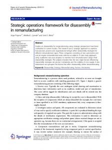
it is advantageous to produce a product with very different arrival and processing characteristics in a separate facility. In our paper, returns arrive to the plant with uncertain timing, and the disassembly and repair process is highly variable. Souza et al. (2001) consider a single-stage production process with no reverse flows, whereas we consider a multi-stage assembly– disassembly process with reverse flows; we contrast our results with theirs in Section 3.6. 3. Model Motivation and Development 3.1. Model Development A firm receives returned products comprised of several parts for remanufacturing. Product returns may be generated via the waste stream, as required by the extended producer responsibility laws, or via a product acquisition management system, where the firm motivates customers to return products of a known quality for a financial incentive and then screens product returns by testing, sorting, and grading operations (see Guide and Van Wassenhove 2001 for a discussion of managing product returns). Returned products are disassembled via a disassembly line, where at each station parts are removed, remanufactured, and placed into an inventory buffer. The yield of reusable recovered parts may be less than 100% due to age, wear, or product upgrade requirements. Assembly orders for new products may be generated by customer orders, or to fill finished good inventories. If available, remanufactured parts are used to assemble new products, otherwise new parts are used. Telecommunications voice switching equipment is an example of routinely remanufactured goods that follow this pattern (Olson 2001), although not the flow design we propose. In voice switching equipment, the end unit is comprised of circuit packs on a frame, and may include other interfacing equipment. During disassembly, parts are removed from the frame until nothing but the frame remains. Frames are then sent to the appropriate stations to add the needed circuit packs and other parts, in order to fill customer orders. In telecommunications equipment, as with many other remanufacturers, the market is extremely lead time sensitive and very small increases in quoted lead times may result in lost sales. 3.2. The Model We consider a product that is assembled by using a flow line that has, for ease of exposition, three assembly steps (parts A, B, and C). The methodology is easily extended to more stations. The order of assembly is C-B-A. We assume that the disassembly sequence is the reverse of the assembly sequence, that is, A-B-C. This is not unreasonable since Nasr, Hughson, Varel, and Bauer (1998) report that over half of all disassembly sequences are simply the reverse of the assembly sequence. There are no yield losses from imperfect remanufacturing processes. We study two main configurations (Figure 1). Under a parallel configuration, there exist two separate dedicated lines: one for assembly and one for disassembly. At each station of the disassembly line, the corresponding part is disassembled, remanufactured, and stored in a buffer to feed the assembly line. For each part, there is an additional buffer originated from a reliable supplier, which is used if there are no remanufactured parts; this buffer is large enough such that the line is never starved. This assumption is necessary for analytic tractability; we relax this assumption in the simulation study of Section 4 and show that our analytic insights are supported by the simulation. Under a mixed configuration, the same station, although with two servers, is used for disassembly, remanufacturing, and assembly of a specific part. All buffers are infinite, including those between stations. For consumer electronics, this simple set of operations (disassembly, testing, and remanufacturing) may be carried out at a single station, and the authors have observed this to be common practice for the remanufacturing of cellular telephones and other electronics items, such as aircraft avionics equipment and telecommunications circuit packs.

MIXED ASSEMBLY AND DISASSEMBLY OPERATIONS FOR REMANUFACTURING

323

FIGURE 1. Configurations for Assembly-Disassembly Lines (Buffers Between Stations Not Shown)

NOTATION assembly arrival rate in products per hour (mean time between assembled products ⫽ 1/␭) squared coefficient of variation (scv) of assembly interarrival time (scv ⫽ variance/ C 2a mean2) ␭r disassembly arrival rate in products per hour (mean time between returned products ⫽ 1/ ␭ r ). We assume that ␭ r ⬍ ␭ , which is consistent with our empirical observations. 2 scv of disassembly interarrival time (scv ⫽ variance/mean2) C a,r p proportion of demand that is filled with remanufactured products ⫽ ␭ r / ␭ i product index: i ⫽ 1 (assembly); i ⫽ 2 (disassembly/remanufacture) j station index: j ⫽ 1, . . . , 6 c number of servers at a station (c ⫽ 1 for parallel line and c ⫽ 2 for mixed line) ␶ ij mean processing time for product i at station j in hours 2 scv of processing time for product i at station j C s,ij ␶ •j mean processing time at station j in hours 2 scv of processing time at station j C s,•j 1/ ␭ ij mean product i interarrival time at station j C 2a,ij scv of interarrival time for product i at station j C 2d,ij scv of interdeparture time for product i at station j 1/ ␭ •j mean product interarrival time at station j C 2a,•j scv of interarrival time at station j C 2d,•j scv of interdeparture time at station j ␳j utilization at station j ⫽ ␭ •j ␶ •j /c W q, j waiting time in queue at station j under first-come-first-serve (FCFS) waiting time in queue at station j for product i when non-preemptive priority (NPP) W NPP q,ij is given to product 1

␭

324

MICHAEL E. KETZENBERG, GILVAN C. SOUZA, AND V. DANIEL R. GUIDE, JR.

There are no distributional assumptions about order interarrival time and product processing time; each station is modeled as a multi-class GI/G/c queue. For a GI/G/c open queuing network, we compute approximate mean flow time using the decomposition approach (Whitt 1983; Bitran and Morabito 1996), which we briefly describe here. Equations (1)–(7) below are equivalent to equations (13), (1), (2), (17), (18), (10), and (7), respectively, in Bitran and Morabito (1996). If products are processed FCFS, then the mean waiting time in queue at station j can be approximated as equal across products, and given by 2 2 , C s,•j , ␭ •j , ␳ j , c兲 ⬇ W q, j 共C a,•j

2 2 ⫹ C s,•j C a,•j 䡠 L q 共 ␳ j , c兲, 2 ␭ •j

(1)

where L q ( ␳ j , c) is the mean queue length of an M/M/c queue with equivalent utilization and number of stations (see, e.g., Buzacott and Shanthikumar 1993, p. 78). The interarrival time parameters are

␭ •j ⫽

冘 ␭ , and

(2)

冘 ␭␭

(3)

ij

i

2 C a,•j ⫽

ij

•j

i

2 C a,ij ,

and the processing time parameters are computed as:

␶ •j ⫽

冘 ␭␭

•j

i

2 C s,•j ⫽

冘 ␭␭ 冉 ␶␶ 冊 i

ij

ij

•j

•j

ij

␶ ij

(4)

2 2 共1 ⫹ C s,ij 兲 ⫺ 1.

(5)

The scv of interdeparture time from station j can be approximated as a function of interarrival and processing time parameters: 2 2 ⫽ 1 ⫹ 共1 ⫺ ␳ 2j 兲共C a,•j ⫺ 1兲 ⫹ C d,•j

␳ 2j

冑c

2 ⫺ 1兲. 共C s,•j

(6)

The splitting of the departure flow among products at station j is: 2 ⫽ C d,ij

␭ ij 2 共C ⫺ 1兲 ⫹ 1. ␭ •j d,•j

(7)

If station k is product i’s next processing station after j, then C 2a,ik ⫽ C 2d,ij . We use superscripts p and m to denote parameters, when different, for the parallel and mixed configurations, respectively. 3.3. Parallel Configuration In the parallel configuration, there is no interaction between the two products at any station. Define the sets A ⫽ {(i, j): i ⫽ 1; j 僆 {1, 2, 3}} (assembly pairs), and D ⫽ {(i, p) j): i ⫽ 2; j 僆 {4, 5, 6}} (disassembly pairs). Then, ␭ (ijp) ⫽ 0 and C 2( a,ij ⫽ 0, for (i, j) ⰻ ( p) 2( p) 2 2( p) 2( p) A 艛 D. Consequently, ␭ •j ⫽ ␭ for j ⫽ 1, 2, 3; C a,•1 ⫽ C a , and C a,•j ⫽ C d,•j⫺1 for j 2( p) ( p) p) ⫽ 2, 3 (where (6) is used to compute C d,•j ). Similarly, ␭ •j ⫽ ␭ r for j ⫽ 4, 5, 6; C 2( a,•4 2 2( p) 2( p) ( p) 2 2 ⫽ C a,r , and C a,•j ⫽ C d,•j⫺1 for j ⫽ 5, 6. Note that ␶ •j ⫽ ␶ ij , and C s,•j ⫽ C s,ij , for (i, j) 僆 A 艛 D. The flow time for assembled products is a direct application of (1) for stations 1 through 3 with c ⫽ 1.

MIXED ASSEMBLY AND DISASSEMBLY OPERATIONS FOR REMANUFACTURING

冘 兵W

325

3

W

共 p兲

⫽

q, j

2共 p兲 2 共C a,•j , C s,1j , ␭ , ␳ 共j p兲, 1兲 ⫹ ␶ 1j其.

(8)

j⫽1

3.4. Mixed Configuration In the mixed configuration, c ⫽ 2 for all stations, product 1 follows the sequence 1-2-3 of stations, and product 2 follows the sequence 3-2-1 (Figure 1). Consequently ␭ (m) 1j ⫽ ␭ and (m) 2(m) ␭ (m) 2j ⫽ ␭ r for all j. Using (4) and (5), we then compute ␶ •j and C s,•j for all j. For product 2 2(m) 2(m) 2(m) 2 2(m) 1, C 2(m) a,11 ⫽ C a , and C a,1j ⫽ C d,1, j⫺1 for j ⫽ 2, 3. For product 2, C a,23 ⫽ C a,r and C a,2j 2(m) ⫽ C d,2, j⫹1 for j ⫽ 1, 2. Using these relationships in (3), (6), and (7) results in a 12 ⫻ 12 linear system of equations, which can be solved to obtain C 2(m) a,•j . If products are processed FCFS, then direct application of (1) with c ⫽ 2 for stations 1 through 3, results in the flow time for assembled products:

冘 兵W 3

W 共m兲 ⫽

q, j

2共m兲 2共m兲 共C a,•j , C s,•j , ␭ ⫹ ␭ r , ␳ 共m兲 j , 2兲 ⫹ ␶ 1j其,

(9)

j⫽1

If we give non-preemptive priority to assembly (product 1), then we need to modify (1) accordingly (see, e.g., Buzacott and Shanthikumar 1993, p. 88): W NPP W q,2j ⫽

NPP q,1j

1 ⫺ ␳ 共m兲 j ⫽ W , and 1 ⫺ ␭␶ 1j / 2 q, j

1 ⫺ ␳ 共m兲 1 j W q, j ⫽ W . 共1 ⫺ ␭␶ 1j / 2兲共1 ⫺ ␭␶ 1j / 2 ⫺ ␭ r␶ 2j / 2兲 1 ⫺ ␭␶ 1j / 2 q, j

(10)

(11)

Consequently, the flow time for assembled products when non-preemptive priority is given to assembly in a mixed line is

冘 兵W 3

W 共m兲,NPP ⫽

2共m兲 2共m兲 共C a,•j , C s,•j , ␭ ⫹ ␭ r , ␳ 共m兲 j , 2兲 ⫹ ␶ 1j其.

NPP q,1j

(12)

j⫽1

3.5. Numerical Study In this section, we perform a comprehensive numerical analysis to establish under which conditions a parallel assembly line is preferred over a mixed assembly line. Our performance measure is the improvement in flow time ⌬ of using a parallel line over a mixed line: ⌬ ⫽ W 共m兲,NPP ⫺ W 共 p兲,

(13)

or, in percentage terms, %⌬ ⫽ 100% 䡠 ⌬/W (m),NPP . We focus on flow time because it is the most critical factor in winning orders stated by the majority of remanufacturing managers (Guide 2000). For ease of exposition, we consider a scenario where all lines are perfectly balanced—all assembly stations have the same processing time (mean and scv), or utilization; analogously for the disassembly stations. We set ␶ 1j ⫽ 10 and ␶ 2j ⫽ 13 for all j, and use a full factorial experimental design for the other parameters shown in Table 1; we justify these choices below. In total, there are 32 䡠 54 ⫽ 5,625 experimental cells. The utilization for assembly operations ␳ j , j ⫽ 1, 2, 3 varies from 0.70 to 0.95; these are high values commonly found in standard manufacturing operations (␭ is computed as ␭ ⫽ ␳ j ␶ 1j , for j ⫽ 1, 2, 3). The proportion of demand that is filled with remanufactured products p varies from 0.25 to 0.75; these are values reported in previous research (Geyer and Van Wassenhove 2000), and determine ␭ r from ␭. The values for C 2a simulate scenarios from

326

MICHAEL E. KETZENBERG, GILVAN C. SOUZA, AND V. DANIEL R. GUIDE, JR. TABLE 1 Experimental Design for Numerical Study Factor

Levels

␳ j , j ⫽ 1, 2, 3 p C 2a 2 C a,r 2 C s,1j 2 C s,2j

0.70, 0.90, 0.95 0.25, 0.50, 0.75 0, 0.25, 0.50, 0.75, 1.0 0, 0.25, 0.50, 0.75, 1.0 0, 0.25, 0.50, 0.75, 1.0 0.50, 0.75, 1.0, 1.5, 2.0

no arrival variability C 2a ⫽ 0 (in a make-to-stock (MTS) environment, a level schedule; in a make-to-order environment, a constant order stream) to random arrivals C 2a ⫽ 1 (Poisson process). 2 ⫽ 0 implies that the firm Regarding the variability of arrivals for returned products, C a,r has a sufficient buffer stock of returned products and that production orders are leveled for the short to intermediate term. This is plausible if the firm has a product acquisition management system in place and there is sufficient demand to justify an assembly line 2 technology (see Guide and Van Wassenhove 2001). At the other extreme, C a,r ⫽ 1 simulates an uncontrolled process for acquisition of used products, perhaps relying on the waste stream, or for a product early in its original product life cycle, where the available supply of used products would be highly uncertain. 2 At one end of the assembly processing time variability spectrum, C s,1j ⫽ 0 implies a 2 process with no variability, for example, an automated process. We point out that C s,1j ⫽0 can be a good approximation to some real processes—a recent empirical study in the auto industry shows values ranging from 0.01 to 0.12 (Inman 1999). At the other extreme of 2 assembly time variability, C s,1j ⫽ 1 implies a highly variable process, for example a labor-intensive process, or a process for highly customized products. Regarding the variabil2 ity of processing time for disassembly and remanufacturing C s,2j , data we collected in several remanufacturing firms suggest that it ranges from 0.5 to 4.0. The lower end of the range is relevant for electronics products (e.g., cellular telephones and avionics) and the upper range for complex mechanical products (e.g., jet turbine engines). Since our research focuses on high volume products, such as consumer electronics, we use in our experimental design the lower end of the range, from 0.5 to 2.0. 3.6. Numerical Results In this section, we summarize the results of the study from Section 3.5; all results are available at http://www.wam.umd.edu/⬃gsouza/mixed_line. Across experiments, %⌬ is positive in only 317 out of 5,625 cells, averaging ⫺296% overall, i.e., on average, the parallel line has a flow time almost four times greater than the mixed line. So, a parallel line outperforms a mixed line in only a small subset of experiments; in most cases, the parallel line has a very poor performance. We now focus on the 317 cells where %⌬ is positive, averaging 19%, to investigate under which conditions the parallel line outperforms the mixed line. Regarding assembly time 2 2 variability, C s,1j ⫽ 0 in 97.8% of cells, and C s,1j ⫽ 0.25 in the remaining 2.2% of cells. 2 Regarding assembly arrival variability, C a ⫽ 0 in 73.2% of cells; C 2a ⫽ 0.25 in 23.0% of cells, and C 2a ⬎ 0.25 in the remaining 3.8% of cells. These results clearly demonstrate that, due to the loss of pooling (that is, the mixed line has two servers per each of its three stations, as opposed to one server per each of its six stations for the parallel line), a parallel assembly line can only be of interest if assembly variability—in both processing and arrival time—is very low. In these cases, (1) shows that queuing time is very low for the parallel assembly

MIXED ASSEMBLY AND DISASSEMBLY OPERATIONS FOR REMANUFACTURING

327

line; thus, the pooling benefit for the mixed line is not high enough to compensate for its higher variability since the performance measure of interest is assembly flow time. We should point out, however, that in these cases where %⌬ ⬎ 0, mean assembly flow times are low (in either configuration), so the values of %⌬ are not as managerially important, i.e., the absolute performance of the mixed line is still good. When the variability in either processing time or arrival time, but not both, is very low, a parallel line is not necessarily preferred, for 2 example, %⌬ is positive in only 27.6% of cells where C s,1j ⫽ 0. 2 The magnitude of ⌬ increases linearly with C s,2j (this can be easily shown, analytically), and increases with ␳ j and p (though not linearly; we elaborate on this in Section 4.3); this is shown in Figure 2. Flow times increase exponentially with ␳ j (see (1)); consequently the magnitude of ⌬ increases with ␳ j . Similarly for p: a higher value of p indicates a higher value of utilization of disassembly operations, hence assembly operations are more “disturbed” by disassembly and remanufacturing operations on a mixed assembly line, and the potential benefits of decoupling the two types of operations by using a parallel configuration are higher. The directional results above are consistent with the focused factory literature: Souza, Wagner, and Whybark (2001), although focused on a single-stage process with no reverse flows, also find that the attractiveness of focused factories (parallel lines) decrease with C 2a 2 2 and C s,1j , and increase with C s,2j , p and ␳ j . In our scenario, the reverse flow of returned products in the mixed line impacts (i) the arrival variability in each station, and (ii) the availability of components for assembly (not captured in this model but studied in Section 4). Thus, the presence of multiple stages and reverse flows does not impact directional focused factory results. Reverse flows and multiple stages appears to limit, however, the environments (in terms of arrival and processing time variability) under which parallel lines are preferred—Souza, Wagner, and Whybark (2001) report several cases where focused factories (parallel lines) improve flow times; we contrast this to our result that parallel lines improve flow times only when assembly variability (in both interarrival and processing time) is very low (scv’s near zero).

2 2 ⫽ 0 and FIGURE 2. Improvement ⌬ in Flow Time of Using a Parallel Line as a Function of C s,2j (C 2a ⫽ C s,1j 2 C a,r ⫽ 1)

328

MICHAEL E. KETZENBERG, GILVAN C. SOUZA, AND V. DANIEL R. GUIDE, JR.

From a managerial perspective, our findings have implications for design engineering efforts to simplify disassembly, remanufacturing, and assembly operations in order to reduce the time required for these tasks and the associated variances. Facility engineers need to consider the entire product life cycle and its impact on product return volumes, whose proxy is p: a facility designed to recover products throughout its life cycle will begin with low values of p in the early stages of new product introduction and as p grows during the original product life cycle, the preferred line configuration will change unless intentional design efforts are made to keep the variances of disassembly and remanufacturing operations low. If these variances are kept in the lower ranges, a mixed line design will be preferred throughout the product’s life cycle. 4. Simulation Two basic assumptions of the analytic model include infinite buffers and no remanufacturing yield loss. While these are necessary to derive analytic insights into the problem, they are not realistic from a practitioner’s standpoint. A primary purpose of the simulation study here is to assess the robustness of the analytic results when these assumptions are relaxed. A secondary purpose is to explore the value of advanced yield information on both assembly and disassembly operations. With remanufacturing yield loss, processing time spent on unrecoverable parts may be greatly reduced with advanced yield information. The German manufacturer Bosch, for example, developed the Data Logger, a computer chip that can be embedded in a power tool to automatically determine if the motor can be recovered (Klausner, Grimm, and Hendrickson 1998). Our research serves as a basis for evaluating the conditions in which investments in such technologies—which provide advanced yield information (smart processing)—are beneficial from a flow time standpoint. Define the capacity ratio k as the ratio between the size of a product buffer b and its average daily requirement. The buffer size is b r ⫽ k ␭ r for remanufactured parts, and is b ⫽ k( ␭ ⫺ ␭ r ) for new parts supplied by the perfectly reliable exogenous supplier. Remanufacturing yield at station j follows a Bernoulli process with probability y j that a part is good and probability 1 ⫺ y j that it is bad and hence unrecoverable. In traditional remanufacturing, actual yield is determined only after the full processing time has transpired at station j. With advanced yield information, actual yield is known instantaneously at station j. To simplify model parameterization, let y j ⫽ y, @ j. The rest of this section is organized as follows: Section 4.1 defines the simulation model, Section 4.2 describes the experimental design, and Section 4.3 presents the results. 4.1. Model The simulation model is similar to the analytic model of Section 3 with exceptions to accommodate discrete events, remanufacturing yield loss, and finite buffers. Each period is an hour and we assume 8 hours in a day. Only at the beginning of each day are new jobs released to the lines and buffers replenished (event 0). The order of events in each hour, other than the first hour, is (1) process jobs, (2) transfer jobs, and (3) set up jobs, described as follows: (0) Job Arrivals and Buffer Replenishment. New jobs arrive to the system at the beginning of every day according to a batch size of mean ␭ and scv C 2a and disassembly jobs arrive 2 every day according to a batch size of mean ␭ r and scv C a,r . The arrival process in the simulation is not a renewal process, as assumed in the analytic model, however, it is consistent with observed remanufacturing practice, where new jobs are initiated at the beginning of the first shift each day. A separate order is created for each job arrival and is placed on the FCFS order queue of the respective job type, where the job type is either assembly or disassembly. At the same time, each job is moved to the queue of the first station for the given job type, according to Figure 1. Finally, new part buffers are replenished when

MIXED ASSEMBLY AND DISASSEMBLY OPERATIONS FOR REMANUFACTURING

329

new jobs are released to the lines—if the quantity in any new parts buffer is less than b, the quantity is brought up to b without delay. (1) Process jobs. Any jobs at station j are either waiting in the priority queue or are in-process with work remaining that is measured in hours. At the beginning of the hour, the time remaining for any in-process jobs is decreased by 1 hour. (2) Transfer new jobs. When the time remaining for a job is zero, the job is finished at that station and is transferred to the next station in line or, in the case the job is completed, it is used to satisfy outstanding orders on a FCFS basis. Specifically, any completed assembly jobs at station 3 are used to satisfy outstanding assembly orders on a FCFS basis. In the case of disassembly, any completed and recovered parts are added to the remanufactured parts bin for the given station. If the disassembly process yields an unrecoverable part, then the part is discarded and the remaining disassembly job is transferred to the next station in the line. (3) Set up new jobs. For each station that is idle, but has jobs waiting in queue, the next job is selected and set up for work. Jobs are selected FCFS, except for the mixed line configuration, where assembly jobs have non-preemptive priority over disassembly jobs. If the next job to be selected is an assembly job and there are no parts available in either the remanufactured parts buffer or the new parts buffer (starving), then a disassembly job will be selected instead. If, however, the next job to be selected is a disassembly job and the remanufactured parts buffer is full (blocking), then no jobs will be selected from the queue. The setup time is zero. When an assembly job is set up at a station, a part is drawn from a buffer, with remanufactured parts having priority over new parts. The processing time for 2 product i at station j is a discrete random variable with mean ␶ ij and scv C s,ij , derived empirically using Excel Solver as follows. (A similar procedure is used for the distribution of batch sizes for the arrival process.) Processing times are integers between 1 and 15 with 2 the corresponding probabilities set to achieve the desired ␶ ij and C s,ij . There is not a unique distribution that satisfies these constraints, but we have empirically observed that the shape of the distribution has negligible or no impact on mean flow times. (Theoretically, mean flow 2 times for a GI/G/c queue can be well approximated using only ␶ ij and C s,ij —see, e.g., Buzacott and Shanthikumar 1993, p. 92.) 4.2. Experimental Design The simulation study uses a factorial design, shown in Table 2, with 24 䡠 32 䡠 5 ⫽ 720 experiments. We duplicate the set of 720 experiments to assess the value of advanced yield information (defined later in Section 4.3.2). Hence, there are a total of 1,440 simulation experiments. 2 2 2 The values for C 2a , C a,r , C s,1j , and C s,2j are a subset of those chosen for the analytic model— given that their impact has already been assessed in Section 3.5—so that we may more fully explore the impact of parameters y and k. The range for y spans the range of values observed in industry where remanufacturing is profitable. For example, the expected

TABLE 2 Experimental Design for Simulation Study Parameter p C 2a 2 C a,r 2 C s,1j 2 C s,2j y k

Levels 0.40, 0.60, 0.80 0.0, 1.0 0.50, 1.0 0.25, 0.50 0.50, 2.0 0.85, 0.90, 0.95 1.50, 1.75, 2.00, 2.25, 2.50

330

MICHAEL E. KETZENBERG, GILVAN C. SOUZA, AND V. DANIEL R. GUIDE, JR.

yield for most parts remanufactured at Xerox is between 0.80 and 0.95; parts with yield below 0.75 are generally considered uneconomical and thus targeted for redesign (Ferrer and Ketzenberg 2001). Across experiments let ␳ j ⫽ 0.80, @j, and ␭ ⫽ 5. Since ␭ and ␳ j are fixed, then both ␶ 1j and ␶ 2j are derived as ␶ 1j ⫽ ␳ j / ␭ and ␶ 2j ⫽ ␳ j / ␭ r . We developed a customized simulation program using the PASCAL programming language. Each experiment is simulated for 2,200 hours and replicated 20 times. The first 200 hours of each replication are set aside for the simulation warm-up period so that statistics are calculated for 2,000 hours in each replication. This 200-hour period was chosen for convenience yet larger than the number of periods necessary for the queues at each station to reach steady state size. The random number streams across all experimental cells are identical for each replication in order to reduce the experiment-wise error. The standard error of any computed statistic averages 2.3% of its mean value, and has a maximum of 3.9%. 4.3. Results Despite their different assumptions, the results from the simulation model generally support the analytic results, suggesting validity for both approaches. The analytic result that ⌬ is positive for only a small fraction of cases—when assembly arrival and processing variability is very low, and disassembly and remanufacturing variability is very high—is 2 ⫽ 0.25, observed in the simulation (1.3% of experimental cells). Only when C 2a ⫽ 0, C s,1j 2 and C s,2j ⫽ 2.0 do we observe positive values for ⌬ that are statistically different from zero (p ⬍ 0.05). Similarly to the analytic results, we observe a trade-off between flow times W (m),NPP and ( p) W , and the mix p (Figure 3). The flow times for Figure 3 were computed by averaging W (m),NPP and W ( p) separately for each level of p across experimental cells. Confirming analytic results, Figure 3 shows that the difference in flow times between the mixed and parallel configurations increases with p. We discuss the impact of finite buffers, remanufacturing yield, and advanced yield information in the sections that follow. 4.3.1. IMPACT OF FINITE BUFFERS AND YIELD LOSS. We illustrate the relationship between the capacity ratio k, remanufacturing yield y, and average flow time in Figure 4. Figure 4 reports

FIGURE 3. Tradeoff Between Flow Time and Mix

MIXED ASSEMBLY AND DISASSEMBLY OPERATIONS FOR REMANUFACTURING

331

FIGURE 4. Relationship Between k, y, and Average Flow Time

average flow time separately for each configuration at each level of k and y; thus, we can observe the main effects of both k and y on flow time, as well as an interaction effect between the two. We discuss each effect in turn below. For either configuration, Figure 4 makes clear that the relationship between average flow time and k exemplifies a service-inventory tradeoff curve. More tightly capacitated buffers lead to more frequent starving and hence longer flow times as illustrated for k ⬍ 2. With large buffers, starving is infrequent so that additional inventory has little impact on long-run average flow times. Note that there is essentially no improvement in flow time of increasing inventory buffer sizes to more than twice a product’s daily requirements. With respect to yield, we observe that the values for W ( p) at each level of y are greater than for W (m),NPP , further corroborating our results with respect to ⌬. Figure 4 also makes clear that both W (m),NPP and W ( p) increase as yield decreases. As yield decreases, the remanufactured content of assemblies decreases. In turn, the quantity of new parts used increases and the rate of starving increases throughout the system— because buffers are capacitated, they become empty more frequently as the demand for new parts increases. In fact, we observe an interaction effect between y and k. Observe in Figure 4 that, as k decreases, the impact of yield increases and the difference in average flow times between each level of y is greater. This occurs because the buffer size k is predicated on both ␭ and ␭ r , but not on y. Hence, as yield decreases, the mean rate of supply to each assembly station decreases, while at the same time the variability of supply increases. In turn, starving occurs more frequently. Hence, we observe that average flow times increase at an increasing rate as both k and y decrease. Interestingly, the impact of yield on average flow time in a mixed configuration is greater than in a parallel configuration. On average, W (m),NPP increases 49% as y decreases from 0.95 to 0.85, while W ( p) increases 32% over the same range. As we have already observed, blocking and starving occurs within mixed and parallel configurations due to finite buffers. Relative to the parallel configuration, the effect of resource pooling in the mixed configuration increases the frequency with which demand exceeds supply for parts, particularly given NPP for assemblies. Hence, the frequency of starving is higher in a mixed configuration and lower remanufacturing yield will tend to exacerbate flow times as a result. It is not surprising that the impact of yield is greater in a mixed configuration than in a parallel configuration, simply because, in a mixed configuration, yield affects all products, while in a parallel case, it only affects disassembly. 4.3.2. VALUE OF ADVANCED YIELD INFORMATION. Using the simulation model, we also explore the value of advanced yield information (VAYI). With advanced yield information,

332

MICHAEL E. KETZENBERG, GILVAN C. SOUZA, AND V. DANIEL R. GUIDE, JR.

part quality is known instantaneously at each disassembly station so that processing time is never wasted on unrecoverable parts. Without advanced yield information, part quality is known only after processing at a station is completed. We measure VAYI as the percent improvement in long-run average flow time that can be achieved with information relative to the case where such information is unavailable. Across experiments, VAYI ranges between 0% and 20%, averaging 5.2%, for the mixed configuration, and ranges between ⫺11% and 39%, averaging 3.8%, for the parallel configuration. The largest improvements occur at lower yields because more time is saved from working on unrecoverable parts. The more interesting result—that the use of yield information in remanufacturing can lead to higher flow times for new assemblies in a parallel configuration—is quite surprising. We observed several cases (more than 50) for the parallel configuration in which the degradation in performance due to advanced yield information was statistically significant at 2 p ⬍ 0.01. These instances occur for experiments where C a,r ⫽ 1.0, p ⫽ 0.8, y ⱕ 0.90, and k ⱕ 2.00. We explain this phenomenon below. Essentially, the use of advanced yield information can cause the system to become unbalanced, and as a result the frequency of blocking and starving increases throughout the system as follows. Yield information eliminates wasted processing time so that disassembly jobs will move through the system faster—across the parallel configuration experiments, the average reduction in flow time for a disassembly job with advanced yield information is 34%. With shorter average flow times, remanufactured parts buffers are replenished more quickly, although the total number of recovered parts at each station does not change. Since remanufactured parts buffers are finite and replenished more quickly with advanced yield 2 is high. When blockinformation, blocking occurs more frequently—particularly when C a,r ing occurs early in the disassembly process (buffer A and station 4) it delays buffers B and C from being replenished. In turn, assembly jobs are often starved for parts, particularly in a tightly capacitated system. We use a representative case to illustrate the phenomenon where 2 2 2 p ⫽ 0.8, C 2a ⫽ 0.0, C a,r ⫽ 1.0, C s,1j ⫽ 0.25, C s,2j ⫽ 0.50, y ⫽ 0.85, and k ⫽ 1.75. In Table 3, we report the fraction of total hours at each station in which we observe blocking and starving in a parallel configuration for this representative case. Note that with advanced yield information, the frequency of both blocking and starving increases. In turn, W (m),NPP increases from 54.9 hours to 60.9 hours; a 10.8% increase. Note that when both starving and blocking occur simultaneously (e.g., starving at station 1 and blocking at station 4), the system must wait until the beginning of the next day, when buffers for new parts are replenished. The lesson is simple: with AYI, the system needs bigger buffers. While advanced yield information can lead to worse performance in a few instances for a parallel configuration, it leads to substantial improvement in other cases. We observe the largest improvements for experiments where p ⫽ 0.8 k ⱖ 2.5, y ⫽ 0.85, and C 2a ⫽ 1.0. Interestingly, while we observe that the average improvement in W (m),NPP (5.2%) due to advanced yield information is greater than corresponding average improvement in W ( p) (3.8%), the range of improvement for W ( p) (⫺11%, 39%) is considerably wider than for W (m),NPP (0%, 20%). In fact, it is somewhat surprising to find that W ( p) is more sensitive TABLE 3 Fraction of Hours at Each Station When Blocking or Starving Is Observed in a Parallel Configuration and VAYI Is Negative, for Representative Case Starving

Without AYI With AYI

Blocking

Station 1

Station 2

Station 3

Station 4

Station 5

Station 6

0.198 0.207

0.188 0.195

0.182 0.193

0.001 0.021

0.000 0.020

0.000 0.014

MIXED ASSEMBLY AND DISASSEMBLY OPERATIONS FOR REMANUFACTURING

333

FIGURE 5. Impact of Capacity Ratio on Average Flow Time With and Without AYI

to advanced yield information than W (m),NPP . In a parallel configuration, the first order effects of using information is limited solely to the disassembly operation, while in a mixed configuration, the first order effects also directly impact the assembly operation. Additional research is needed to understand the dynamics for these results. For either type of configuration, however, the use of advanced information has the effect of shifting the service-inventory tradeoff curve. In Figure 5, we illustrate the relationship between the capacity ratio and average flow time for both configurations and for the cases with and without advanced yield information. Notice that with advanced yield information, average flow time improves for every level of k, but note also that the effect of AYI is much smaller, on average, than the difference between the mixed and parallel lines. 5. Conclusions We study mixed assembly– disassembly line configurations when components of a product can be supplied by disassembly and remanufacturing (DR) operations, and the disassembly sequence is exactly the reverse of the assembly sequence. Under the mixed line configuration, DR and assembly are performed in the same line—assembly operations flow downstream whereas DR operations flow upstream. Under the parallel configuration, there are separate lines for assembly and DR. This problem differs from traditional assembly line design because of the reverse DR flow that provides parts to the forward assembly flow. Under which conditions is a particular configuration preferred in terms of mean assembly time? To answer this question, we propose an analytic model that assumes infinite buffers between stations, and an alternative reliable supplier with zero lead time for each part; we relax these assumptions in a simulation. Our analytic model is similar to the focused factory model by Souza, Wagner, and Whybark (2001), except that our model involves multiple stages and a reverse flow of products. Despite these differences, however, we obtain similar directional insights: the attractiveness of parallel lines (or focused factories) decrease with the variability of assembly interarrival and processing times, and increase with the variability of DR processing time, the percentage of demand that is met with remanufactured parts, and line utilization. Our

334

MICHAEL E. KETZENBERG, GILVAN C. SOUZA, AND V. DANIEL R. GUIDE, JR.

extensive numerical study with parameters values drawn from remanufacturing practice, however, provides a key new insight: due to a loss of pooling, parallel lines are preferred over mixed lines only in a very small subset of cases—when the variability of assembly interarrival and processing times are very low (scv’s near zero), and the magnitude of these benefits increase with variability in DR processing time. This key insight is supported by simulation results where buffers are finite, and there is yield in remanufacturing process. The simulation also provides some key insights into the impact of finite buffers, the impact of yield loss, and the value of advanced yield information. Our findings show that finite inventory buffers equal to two days production requirements provide the same flow times as infinite buffers, and that even relatively small finite buffers offer significant improvements in flow times. As yield loss increases, average flow times increase and the increase in flow times is more pronounced for mixed line configurations. Also, as yield loss increases, the buffer size necessary to maintain a given flow time level increases. Managers can influence the known yield by first working with design engineers to develop products with a finite, known number of uses, as is the case with power transformers used in Xerox photocopiers. If the number of useful lives is tracked in a database system, managers can plan on replacing the part the n th time the product is returned. However, this may only be useful where products may be remanufactured more than once. Managers may also foster the development of technology to facilitate advanced yield information, as with the Bosch electronic data logger system. In general, advanced yield information decreases flow times, although in some very special cases it increases flow times, a surprising result. In these very special cases, the use of advanced yield information may result in line imbalances, and these imbalances increase the starvation and blocking of jobs throughout the system, increasing flow times. Further research is certainly needed to fully explore these results in detail.1 1 We would like to recognize that the initial ideas for this project were generated during the first workshop on the Business Aspects of Closed-Loop Supply Chains in 2001, sponsored by the Carnegie Bosch Institute. Also, we thank two anonymous referees and the editors for the special issue for their comments and suggestions on earlier versions of this paper.

References BITRAN, G. AND R. MORABITO (1996), “Open Queuing Networks: Optimization and Performance Evaluation Models for Discrete Manufacturing Systems,” Production and Operations Management, 5, 2, 163–193. BUZACOTT, J. AND G. SHANTHIKUMAR (1993), Stochastic Models of Manufacturing Systems, Prentice Hall, Englewood Cliffs, New Jersey. CHOW, W. M. (1990), Assembly Line Design: Methodology and Applications, Marcel Dekker, New York, New York. FERRER, G. AND M. KETZENBERG (2001), “Value of Information in Remanufacturing Complex Products,” Kenan Flagler Business School Working Paper, University of North Carolina. FLEISCHMANN, M. (2001), “Quantitative Models for Reverse Logistics,” Lecture Notes in Economics and Mathematical Systems, Volume 501, Springer-Verlag. Berlin. GEYER, R. AND L. N. VAN WASSENHOVE (2000), “Product Take-Back and Component Reuse,” The Center for Integrated Manufacturing and Service Operations, INSEAD R&D Working Paper 2000/34/TM/CIMSO 12. GUIDE, JR., V. D. R. (2000), “Production Planning and Control for Remanufacturing: Industry Practice and Research Needs,” Journal of Operations Management, 18, 467– 483. GUIDE, JR., V. D. R., V. JAYARAMAN, R. SRIVASTAVA, AND W. C. BENTON (2000), “Supply Chain Management for Recoverable Manufacturing Systems,” Interfaces, 30, 3, 125–142. ———, ———, AND R. SRIVASTAVA (1999), “Production Planning and Control for Remanufacturing: A State-ofthe-Art Survey,” Robotics and Computer-Integrated Manufacturing, 15, 3, 221–230. ——— AND R. SRIVASTAVA (1998), “Inventory Buffers in Recoverable Manufacturing,” Journal of Operations Management, 16, 551–568. GUIDE, JR., V. D. R. AND L. N. VAN WASSENHOVE (2000), “Closed-Loop Supply Chains,” INSEAD R&D Working Paper 2000/75/TM. ——— AND ——— (2001), “Managing Product Returns for Remanufacturing,” Production and Operations Management, 10, 2, 142–155.

MIXED ASSEMBLY AND DISASSEMBLY OPERATIONS FOR REMANUFACTURING

335

GUNGOR, A. AND S. M. GUPTA (2001), “Disassembly Sequence Plan Generation Using a Branch and Bound Algorithm,” International Journal of Production Research, 39, 481–509. INMAN, R. (1999), “Empirical Evaluation of Exponential and Independence Assumptions in Queueing Models of Manufacturing Systems,” Production and Operations Management, 8, 4, 409 – 432. KLAUSNER, M., W. M. GRIMM, AND C. HENDRICKSON (1998), “Reuse of Electric Motors in Consumer Products,” Journal of Industrial Ecology, 2, 2, 89 –102. LUND, R. (1984), “Remanufacturing,” Technology Review, 19 –29. ——— (1998), Remanufacturing: An American Resource. Fifth International Congress for Environmentally Conscious Design and Manufacturing, Rochester Institute of Technology. NASR, N., C. HUGHSON, E. VAREL, AND R. BAUER (1998), “State-of-the-art Assessment of Remanufacturing Technology,” Rochester Institute of Technology, National Center for Remanufacturing, Rochester, New York. OLSON, D. (2001), Special Customer Operations, Lucent Technologies, Private communication with the authors. SOUZA, G. C., M. KETZENBERG, AND V. D. R. GUIDE, JR. (2002), “Capacitated Remanufacturing with Service Level Constraints,” Production and Operations Management, 11, 2, 231–248. ———, H. M. WAGNER, AND D. C. WHYBARK (2001), “Evaluating Focused Factory Benefits with Queuing Theory,” European Journal of Operational Research, 128, 597– 610. WHITT, W. (1983), “The Queuing Network Analyzer,” Bell Syst. Tech. J., 62, 2817–2843.

Michael E. Ketzenberg is an assistant professor of operations management in the College of Business at Colorado State University. Dr. Ketzenberg earned his Ph.D. from the University of North Carolina at Chapel Hill. His research interests include remanufacturing, supply chain management, and value of information. His work has appeared in several journals, including Production and Operations Management, Harvard Business Review, Journal of Operations Management, and International Journal of Production Economics. Gilvan C. Souza is an assistant professor of management science in the Robert H. Smith School of Business at the University of Maryland. Dr. Souza earned his Ph.D. from the University of North Carolina at Chapel Hill. His research interests include remanufacturing, management of technology, and supply chain management. His work has appeared or is forthcoming in Production and Operations Management, Management Science, European Journal of Operational Research, and International Journal of Production Research. V. Daniel R. Guide, Jr. joined the faculty in the Department of Supply Chain & Information Systems in the Smeal College of Business Administration, The Pennsylvania State University in the fall of 2002. He was a visiting research scholar at INSEAD from 2001–2003. Professor Guide’s research is focused on the development and control of closed-loop supply chains, time-based models for commercial product returns, remanufacturing, and industrial ecology. His research has appeared in numerous academic and managerial journals, including Manufacturing & Service Operations Management, Harvard Business Review, Interfaces, and this journal. Professor Guide’s research has been supported by grants from the Carnegie Bosch Institute and the National Science Foundation. He also regularly works and consults with global organizations (including the U.S. Navy, HewlettPackard, Robert Bosch Tool Company, and Lucent) on a variety of supply chain problems.