imizing the sum of weighted absolute residuals through linear programming meth- ods. Recently, an ..... (Kollo and Srivastava, 2004). 3 Simulation Study.
The International Journal of Biostatistics Volume 5, Issue 1
2009
Article 28
Mixed-Effects Models for Conditional Quantiles with Longitudinal Data Yuan Liu, Medical University of South Carolina Matteo Bottai, University of South Carolina
Recommended Citation: Liu, Yuan and Bottai, Matteo (2009) "Mixed-Effects Models for Conditional Quantiles with Longitudinal Data," The International Journal of Biostatistics: Vol. 5: Iss. 1, Article 28. DOI: 10.2202/1557-4679.1186
Unauthenticated Download Date | 10/18/18 8:34 AM
Mixed-Effects Models for Conditional Quantiles with Longitudinal Data Yuan Liu and Matteo Bottai
Abstract We propose a regression method for the estimation of conditional quantiles of a continuous response variable given a set of covariates when the data are dependent. Along with fixed regression coefficients, we introduce random coefficients which we assume to follow a form of multivariate Laplace distribution. In a simulation study, the proposed quantile mixed-effects regression is shown to model the dependence among longitudinal data correctly and estimate the fixed effects efficiently. It performs similarly to the linear mixed model at the central location when the regression errors are symmetrically distributed, but provides more efficient estimates when the errors are over-dispersed. At the same time, it allows the estimation at different locations of conditional distribution, which conveys a comprehensive understanding of data. We illustrate an application to clinical data where the outcome variable of interest is bounded within a closed interval. KEYWORDS: asymmetric Laplace distribution, longitudinal data, mixed-effects model, Monte Carlo Expectation Maximisation (MCEM) algorithm, multivariate Laplace distribution, quantile regression Author Notes: We thank the two anonymous reviewers for their insightful comments and Dr. Sharon Yeatts for her help with the editing.
Unauthenticated Download Date | 10/18/18 8:34 AM
Liu and Bottai: Quantile Mixed-Effect Model
1 Introduction Popularized by Koenker and Bassett (1978), quantile regression has gradually become a well established technique in a wide range of applications. It represents an important complement to the classic mean regression and characterizes the whole conditional distribution of a response variable given a set of covariates. Robustness against outliers, efficiency for a wide range of error distributions, and equivariance to monotone transformation are some of the other desirable features of quantile regression. Median regression, a special case of quantile regression and a type of robust regression, has been familiar to most researchers. Quantile regression has recently been applied is a variety of areas, including economics (Machado and Mata, 2005; Angrist et al., 2006), medicine/public health (Austin and Schull, 2003; Austin et al., 2005; Wei et al., 2006), ecology (Cade et al., 2005), survival data analysis (Yin and Cai, 2005) and microarray data analysis (Sohn et al., 2008; Li and Zhu, 2007; Huang et al., 2008). For more details about the quantile regression approach, one can refer to Buchinsky (1998), Koenker and Hallock (2001), Yu et al. (2003), and Koenker (2005). In the case of classic quantile regression, there are very few assumptions about the form of error distribution, and the estimation of parameters is obtained by minimizing the sum of weighted absolute residuals through linear programming methods. Recently, an asymmetric Laplace distribution (ALD), which is characterized by a peak at the mode and thick tails, has been used in Bayesian quantile regression for error distribution (Yu and Zhang, 2005; Yu and Moyeed, 2001). The connection between maximizing a likelihood function composed of independently distributed ALD and minimisation of the objective function in quantile regression was shown by Yu and Moyeed (2001) and used to develop the likelihood ratio test for quantile regression (Koenker and Machado, 1999), and to apply quantile regression to longitudinal data (Geraci and Bottai, 2007). In the mean regression, a similar connection exists between MLE based on normal distribution and least-squares estimation. Kotz et al. (2001) and Kozubowski and Nadarajah (2008) reviewed several different forms of the Laplace distribution. In this paper, we focus on exploring the use of quantile regression for analysis of longitudinal data. These data are characterized by repeated measurements on the same subject over time, as may be collected in clinical trials, epidemiologic studies, etc. By using the connection between ALD and quantile regression, we develop a likelihood-based approach to estimate parameters of conditional quantile functions with the random effects by adopting an ALD for the residual errors and a multivariate distribution for the random effects that is not restricted to be normal. This quantile mixed-effects model is analogous to the linear mixed model (Verbeke and Molenberghs, 2000; Demidenko, 2004). The within-subject dependence 1
Unauthenticated Download Date | 10/18/18 8:34 AM
The International Journal of Biostatistics, Vol. 5 [2009], Iss. 1, Art. 28
among data is taken into account through incorporation of random effects to avoid bias in the parameter estimate. The proposed approach allows the estimation at different quantiles of conditional distribution, and hence leads to a robust estimation of parameters and conveys a comprehensive understanding of data. There is a relatively small amount of literature about the extension of quantile regression to longitudinal data or dependent data. Three types of models can be identified among them: the marginal model, penalized model and conditional model. Jung (1996) proposed quasi-likelihood based estimating equations for median regression, and based on Jung’s work, Lipsitz et al. (1997) described a weighted GEE model in quantile regression for longitudinal data with random drop-off. Karlsson (2008) examined a weighted version of quantile regression estimator adjusted to the case of nonlinear longitudinal data. These methods are basically marginal models which capture the overall trend among all subjects for a given quantile. Koenker (2004) proposed a penalized quantile regression with a large number of subject-specific fixed effects, in which the inflation effect was controlled by a regularization, or shrinkage, whose degree needs to be chosen suitably. Geraci and Bottai (2007) proposed a conditional model for quantile regression with random intercept. In this paper, we generalize the conditional model proposed by Geraci and Bottai (2007) and a quantile regression with multiple random effects is developed. In addition, instead of normal distribution for the random effects, heavy-tailed distributions are usually considered to handle outliers and unduly large observations in robust mixed models (Lange et al., 1989; Pinheiro et al., 2001; Song et al., 2007). Inspired by the robustness of quantile regression and heavy-tailed property for ALD, we describe and evaluate the use of a symmetric multivariate Laplace distribution (Kotz et al., 2001) for the random effects, which is characterized by peak at zeros and thick tails on the edges. Multivariate Laplace distribution has been mainly used in speech and image data, and to the best of our knowledge it is the first time that this distribution is being considered for the random effects in a mixed model. This paper is organized as follows: Section 2 gives the connection between ALD and quantile regression, the quantile mixed-effects model, a proposed semiparametric Monte Carlo Expectation Maximization (MCEM) algorithm for point estimation, and an introduction to a multivariate Laplace distribution; Section 3 conducts a simulation study aimed to evaluate the performance of the proposed model; Section 4 illustrates an application to clinical trial data; Section 5 makes a conclusion.
DOI: 10.2202/1557-4679.1186
2
Unauthenticated Download Date | 10/18/18 8:34 AM
Liu and Bottai: Quantile Mixed-Effect Model
2 Model and Method 2.1 Independent Data Suppose (xTi , yi), i = 1, . . . , N, is an independent random sample from some population, where xi is a p × 1 vector of regressors and yi is a scalar response variable with conditional cumulative distribution function Fy , whose shape is unspecified. Following Koenker and Bassett (1978), the τ -th quantile of data is modeled as Qyi (τ |xi ) = xTi βτ ,
i = 1, . . . , N,
where τ ∈ (0, 1), Qyi (·) ≡ Fy−1 (·), and βτ ∈ Rp is a column vector of unknown i fixed parameters with length p. Alternatively, the above expression can be rewritten as yi = xTi βτ + ǫi , with Qǫi (τ |xi ) = 0, where ǫi is the error term whose distribution is restricted to have the τ -th quantile to be zero. Through a numerical method, e.g. linear programming, the estimator βˆτ is obtained by solving βˆτ = arg min β∈Rp
N X
ρτ (yi − xTi βτ ),
(1)
i=1
where ρτ (v) = v(τ − I(v 6 0)) is the loss function with v being a real number and I(·) is the indicator function. For a special case of τ = 0.5 (median regression), equation (1) simplifies to βˆ0.5 = arg min β∈Rp
N X
|yi − xTi β0.5 |.
i=1
The parameter βτ and its estimator βˆτ depend on the quantile τ . For simplicity, we will omit the subscript in the remainder of the paper. A three-parameter ALD (Yu and Zhang, 2005) provides a natural link between minimization of the sum of weighted absolute residuals in equation (1) and the maximum likelihood theory. Other forms of Laplace distribution were summarised by Kotz et al. (2001) and Kozubowski and Nadarajah (2008). A random variable Y follows an ALD if its corresponding probability density is given by � � �� τ (1 − τ ) y−µ exp −ρτ , (2) f (y|µ, σ, τ ) = σ σ
where ρτ (v) is defined in equation (1), σ > 0 is the scale parameter, and −∞ < µ < +∞ is the location parameter which is also the mode and the τ -th quantile of 3
Unauthenticated Download Date | 10/18/18 8:34 AM
The International Journal of Biostatistics, Vol. 5 [2009], Iss. 1, Art. 28
y. Let µi = xTi β, and for any given value of τ , we assume that ǫi ∼ ALD(0, σ, τ ), which restricts the τ -th quantile of residuals to be zero. Then the likelihood for N independent observations is written, ( N ) X � y i − xT β � i L(β, σ; y, τ ) ∝ σ −N exp − ρτ . (3) σ i=1 Considering σ a nuisance parameter, the maximisation of the likelihood in (3) with respect to the parameter β is equivalent to the minimisation of the objective function in (1).
2.2 Longitudinal Data Consider longitudinal data with repeated measurements in the form (yij , xTij ), for j = 1, . . . , ni , and i = 1, . . . , N, where yij is the jth scalar measurement of a continuous random variable on the ith subject, xTij are row p−vectors of a known design matrix and β is a p × 1 vector of fixed regression coefficients. We follow the similar notation as the linear-mixed model and define the linear mixed-effects quantile function of response yij as yij = xTij β + zTij ui + ǫij ,
with Qǫij (τ |xij , ui ) = 0,
(4)
where zij is a q × 1 subset of xij with random effects; ui is a q × 1 vector of random regression coefficients; the error term ǫij , for j = 1, . . . , ni and i = 1, . . . , N, is assumed to be independently distributed as ALD. The random regression coefficents ui , for i = 1, . . . , N, which account for the correlation among observations, are assumed to be mutually independent and to follow some multivariate distribution fu (0, Σ). We discuss the choice of the distribution for random effects, fu (0, Σ), in section 2.5. We also assume independence between ui and ǫij and between the random regression coefficients ui and the explanatory variables xTij . The conditional density function of yij |ui can be written as � � �� τ (1 − τ ) yij − µij f (yij |ui , xij ; β, σ) = exp −ρτ , σ σ where µij = xTij β + zTij ui is the linear predictor of the τ th quantile function, and τ is fixed and known. Q i Let f (yi |ui , xi ; β, σ) = nj=1 f (yij |ui , xij ; β, σ) be the density for the ith subject conditional on the random effect ui , where yi = (yi1 , . . . , yini )T and xi =
DOI: 10.2202/1557-4679.1186
4
Unauthenticated Download Date | 10/18/18 8:34 AM
Liu and Bottai: Quantile Mixed-Effect Model
(xi1 , . . . , xini )T . The complete data density of (yi , ui ), for i = 1, . . . , N, is then given by f (yi , ui |xi ; η) = f (yi |ui , xi ; β, σ)f (ui |xi ; Σ) = f (yi |ui , xi ; β, σ)f (ui |Σ), where we assume that ui is independent of xi , f (ui |Σ) is the density of ui , and η = (β, σ, Σ) is the parameter of interest. If we let y = (y1 , . . . , yN ), x = (x1 , . . . , xN ) and u = (u1 , . . . , uN ), the joint density of (y, u) based on N subjects is given by f (y, u|x; η) =
N Y
f (yi |ui , xi ; β, σ)f (ui |Σ).
(5)
i=1
For simplicity, in the next section we will use f (y, u|η) and f (y|η) to denote f (y, u|x; η) and f (y|x; η) .
2.3 Estimation We obtain the maximum likelihood estimates for the parameter η by maximising the marginal density f (y|η), which is calculated by integrating out the random effects u R in equation (5). That is, L(η; y) = f (y|u; η)f (u; Σ)du. Only under limited cases, however, is a closed form solution available; generally, this integral is intractable. We propose a Monte Carlo Expectation Maximisation (MCEM) algorithm, which has been widely applied to generalized linear mixed models (Booth and Hobert, 1999). Within this algorithm, random effects are considered as unobserved, missing values and a simulation method is used to evaluate the intractable integral in the Estep. 2.3.1 E-step We write the E-step for the ith subject at iteration (t + 1) Oi(η|η (t) ) = E{l(η; yi , ui )|yi ; η (t) } Z = {log f (yi |β, ui , σ) + log f (ui |Σ)}f (ui |yi , η (t) )dui ,
(6)
where η (t) = (β (t) , σ (t) , Σ(t) ), l(η; yi , ui ) is the log likelihood for the ith subject, and the expectation is taken with respect to the distribution of the unobserved data ui given the observed data yi , whose density is f (ui |yi , η (t) ) ∝ f (yi |ui ; β (t) , σ (t) )f (ui |Σ(t) ).
(7) 5
Unauthenticated Download Date | 10/18/18 8:34 AM
The International Journal of Biostatistics, Vol. 5 [2009], Iss. 1, Art. 28
By drawing a random sample vi = (vi1 , . . . , vimi ) of size mi from the conditional distribution of f (ui |yi , η (t) ) in (7), the expectation in (6) can be approximated by mi 1 X (t) Oi (η|η ) ≈ {log f (yi |vik ; β, σ) + log f (vik |Σ)}. (8) mi k=1
Based on the assumption that the observations are independent across subject, the marginal density of log f (y|η) is approximately O(η|η (t) ) ≈ ≈
N X i=1 N X i=1
Oi (η|η (t) ) mi 1 X {log f (yi |vik ; β, σ) + log f (vik |Σ)}. mi k=1
(9)
The Monte Carlo M-step is usually relatively simple as pointed out by McCulloch (1994). The reason is that O(η|η (t) ) in equation (9) is the sum of a likelihood involving only β and σ in the first term and a second term involving only Σ. In the first term, if we let y˜ijk = yij − zTij vik , then we may consider y˜ijk to be independent, and the maximisation of (9) with respect to β and σ leads to a linear quantile regression with response variable y˜ijk . The maximisation with respect to Σ can sometimes be written in closed form depending on the distribution of the random effects. 2.3.2 M-step To obtain the maximum likelihood estimate of the parameter η for the τ th quantile function, we propose the following iterative procedure: Step 1: Initialize the parameters η (t) = (β (t) , σ (t) , Σ(t) ), set t = 0 and substitute η (t) in (7); (t)
(t)
Step 2: For each subject i = 1, . . . , N, independently draw a sample vi = (vi1 , . . . , (t) vimi ) for k = 1, . . . , mi , from equation (7) with sample size mi by a MCMC sample, e.g. via the Gibbs sampler with the adaptive rejection sampling algorithm (Gilks et al., 1995). Step 3: Solve β
(t+1)
DOI: 10.2202/1557-4679.1186
mi X ni N X 1 X (t) = arg min ρτ (y˜ikj − xTij β), β∈B m i i=1 k=1 j=1
6
Unauthenticated Download Date | 10/18/18 8:34 AM
Liu and Bottai: Quantile Mixed-Effect Model (t)
(t)
where y˜ikj = yij − zTij vik . Set σ
(t+1)
= PN
1
i=1
and
ni mi
mi X ni N X X
(t)
ρτ (y˜ikj − xTij β (t+1) )
i=1 k=1 j=1
b (t) , . . . , v(t) ), Σ(t+1) = Φ(v i N
b is the maximum likelihood estimate of Σ, which depends on the where Φ distribution of random effects;
Step 4: Set t = t + 1 and repeat steps 1 − 3 until the parameter η achieves convergence. In step 2, Monte Carlo random samples for random effects are generated by a Gibbs sampler and used to approximate the E-step, and the minimisation problem in step 3 is equivalent to a weighted quantile regression with an offset. Then, at each iteration, η (t+1) is the maximum likelihood estimate of η, given η (t) . The choice of the Monte Carlo sample size mi and convergence criteria are important issues in the implementation of the MCEM algorithm. It is well known that the simulation size mi should be increased with the number of iterations. Several approaches have been proposed to increase the simulation size over iterations. Booth and Hobert (1999) suggested a rule for increasing the number of simulations when the change in the parameter value is swamped by Monte Carlo error, as well as a rule for stopping when the change in the parameter estimates relative to their standard errors is small enough. Instead, Eickhoff et al. (2004) proposed a likelihood-distance-based algorithm, in which the change in the estimated log likelihood over iterations is evaluated, and the algorithm is stopped when such a likelihood distance is less than a certain small number δ with probability larger than 1 − ǫ (e.g., ǫ = 0.05 or 0.01). We adopt Eickhoff’s algorithm to assess convergence of the MCEM algorithm, since the likelihood at each iteration can be approximated by random samples directly. The final estimated log likelihood can also be used to calcualte the AIC to evaluate the model fit.
2.4 Confidence Intervals for Parameters Construction of confidence intervals for the parameters is usually based on the asymptotic normality of the maximum likelihood estimator (MLE). The asymptotic theory for quantile regression is well studied, but the development of convenient inference procedures has been challenging, as the asymptotic covariance matrix of quantile estimates involves the unknown error density function which cannot be 7
Unauthenticated Download Date | 10/18/18 8:34 AM
The International Journal of Biostatistics, Vol. 5 [2009], Iss. 1, Art. 28
estimated reliably. In our case, the error term has been set to be ALD, and for a given τ , the mode of ALD is located at the τ -th quantile of residuals. Maximizing the likelihood leads to unbiased point estimate, but ALD may not represent the true distribution of error density. At the same time the density function f (y|η) might not be differentiable with respect to η. Alternatively, some other methods are available to provide inference for quantile regression with longitudinal data, such as the rank score test proposed by Wang and Fygenson (2009) recently, and the block bootstrap method which has been applied in the works of Buchinsky (1995) and Lipsitz et al. (1997). In this study, we consider the latter method to construct tests and the confidence intervals for βτ . The bootstrap method has been widely used in applications of quantile regression. To retain the dependent structure in a longitudinal data, independent subjects are assumed and the xy-pairs from each subject {(yi , xi ), for i = 1, . . . , N} are treated as basic resampling units and sampled from original data with replacement B times. The practical question about choosing the number of replications B was addressed by Andrews and Buchinsky (2000, 2001).
2.5 Multivariate Laplace Distribution for Random Effects In this section we focus on the distribution for the random effects in our model. Random effects in the linear mixed model are typically assumed to follow a multivariate normal distribution, which sometimes is believed to be too restrictive to represent the data and vulnerable to outliers. Multivariate Student’s t distribution is a classic alternative, which is useful when the data are over dispersed with respect to the normal distribution. Other multivariate distributions with heavier tails than normal may also provide alternatives. Inspired by the robustness property of the Laplace distribution, we consider a multivariate Laplace distribution. As discussed by Kotz et al. (2001), let X be a q-dimensional, zero-mean Gaussian variable with covariance matrix equal to Σ, and Z be a standard exponential variable which is independent of X; then the representation Y = mZ + Z1/2 X is distributed as multivariate Laplace distribution with parameter m and Σ and denoted as Y ∼ ALq (m, Σ), whose density can be expressed as
f (y; m, Σ) =
2ey
T Σ−1 m
�
yT Σ−1 y 2 + mT Σ−1 m
�ν/2
(2π)q/2 |Σ|1/2 np o T −1 T −1 ×Kν (2 + m Σ m)(y Σ y) ,
(10)
where m is a q-vector, Σ is a q × q covariance matrix, ν = (2 − q)/2 and Kν (u) is the modified Bessel function of the third kind which is given by DOI: 10.2202/1557-4679.1186
8
Unauthenticated Download Date | 10/18/18 8:34 AM
Liu and Bottai: Quantile Mixed-Effect Model
� � Z 1 � u �ν ∞ −λ−1 u2 Kν (u) = t exp −t − dt, u > 0. 2 2 4t 1 The density in equation (10) represents a series of skewed multivariate distribution with E(Y) = m and COV (Y) = Σ + mmT , in which parameter m controls both location and skewness. For m = 0, it simplifies to a symmetric multivariate Laplace distribution which is elliptically contoured. Also, when q = 1, equation (10) is another form of asymmetric Laplace distribution discussed by Kozubowski and Nadarajah (2008). Kotz et al. (2001, page 233) showed the heavier tail of symmetric bivariate Laplace distribution relative to a Gaussian bivariate density under same setting of m and Σ. Because of the availability of the correlation matrix, Lindsey and Lindsey (2006) applied it to model dependence among repeated measurements data. Eltoft et al. (2006) presented a similar symmetric multivariate Laplace distribution with application of speech and image data. In our quantile mixed-effects model, for a given quantile τ , the random effects are assumed to be distributed around βτ with zero-mean, so a symmetric multivariate Laplace distribution is adopted for the random effects in model (5) as
f (ui ; Σ) =
2 (2π)q/2 |Σ|1/2
�
uTi Σ−1 ui 2
�ν/2
Kν
�q
2(uTi Σ−1 ui )
�
.
(11)
The implementation of this distribution into the MCEM algorithm described in section 2.3 is straightforward, and the modified Bessel function in the likelihood is available in the statistical software R. After generating random sample for random (t) (t) effects (vi , . . . , vN ) in step 2 of the MCEM algorithm, we are able to get the b (t+1) by an iterative EM-type approach (Eltoft et maximum likelihood estimate Σ b (t+1) = al., 2006). Alternatively, by method of moments, we can calculate that Σ P (t) (t)T N 1 (Kollo and Srivastava, 2004). i=1 vi vi N
3 Simulation Study We evaluate the performance of the proposed quantile mixed-effects model at several quantiles of data under different data-generating scenarios. The probability distributions for the error term are generated from the Normal, the Student’s T3 and the χ22 distribution, and the latter two represent over-dispersed data and skewed data respectively. The probability distributions for the random effects are selected from either the Normal or the T3 distribution, and the correlation among the random effects is set to be zero. Hence there are a total of six combinations of distribution for the error term and the random effects.
9
Unauthenticated Download Date | 10/18/18 8:34 AM
The International Journal of Biostatistics, Vol. 5 [2009], Iss. 1, Art. 28
We use N = 20 subjects and ni = n = 20, for i = 1, . . . , N, measurements within each subject. The data are generated by the model yij = 1 + 2xij + u0i + u1i xij + ǫij ,
j = 1, . . . , 20,
i = 1, . . . , 20, (12)
where xij is the independent variable generated from a uniform distribution between 0 and 20. The random effects for intercept, u0i , and slope, u1i , and the error term, ǫij , are independently generated and the selected distribution is standardized to have mean zero and variance one. In each scenario, 1000 simulated data sets are generated, and for each data set, we estimate the fixed regression coefficients β for three different quantile functions, τ = (0.25, 0.50, 0.75), by using the proposed model in which a Laplace distribution for error term and a multivariate Laplace distribution for random effects are used to construct the likelihood. For comparison, we also provide the parameters estimated by the linear mixed model (LMM). Based on 1000 Monte Carlo replications, the bias and variance of the estimators of the fixed regression coefficients, β0 and β1 , for each quantile τ are calculated as Bias = β¯l − βl 1000 1 X ˆ(k) ¯ 2 Variance = (β − βl ) , 1000 k=1 l
P ˆ(k) where β¯l = 1000 k=1 βl /1000 and βl , l = 0, 1 are the quantile-dependent true values of the intercept and slope. According to the data-generating procedure, the true value of β0 is obtained by adding the τ -th quantile value of standardized error distribution to the true intercept value, which is 1 in this simulation study. The true value β1 = 2 is constant across quantiles. The left panel of Figure 1 shows the scatter plot of the data from a single simulated data set generated from standardized normal distributions for both the error term and the random effects. The variance of y increases along with x. First we erroneously treat these as independent data and estimate the slope of y given x by classical linear quantile regressions for 9 quantiles, τ = 0.1, 0.2, . . . , 0.9. The estimated slope βˆ1 increases along with τ (black dots in right panel). Then we apply the proposed quantile mixed-effects model. The estimates βˆ1 are consistently near the true value (hollow triangles in right panel). This indicates that, for longitudinal data, the dependence within subjects should be accounted for to avoid serious bias in the estimation of quantile regression models. Table 1 summarizes the results from six scenarios. The fixed regression slope ˆ β1 estimated by the proposed quantile mixed-effects model does not vary across DOI: 10.2202/1557-4679.1186
10
Unauthenticated Download Date | 10/18/18 8:34 AM
Liu and Bottai: Quantile Mixed-Effect Model
60
2.4
50
2.2
40
2.0
y 30
^ β1 1.8
20
1.6 1.4
10
1.2
0 0
5
10 x
15
20
0.0
0.2
0.4
0.6
0.8
1.0
τ
Figure 1: A plot of simulated data generated by normal distributions for both the error term and the random effects (left panel). On the right panel, the black dots indicate the estimated slope of y given x by assuming independent observations at 9 quantiles (τ = 0.1, 0.2, . . . , 0.9), and the hollow triangles indicate the estimated slope by the proposed quantile mixed-effects model. quantiles and is consistently around its true value with small bias and variance in all the six scenarios. For the scenarios with symmetric error distributions (ǫ ∼ Normal, ǫ ∼ T3 ), in which the mean and median are equal, we compare the median mixed-effects model Q0.50 with LMM. The two methods showed comparable bias and variance. The point estimates of the fixed regression intercept βˆ0 vary the quantiles and capture the location of the different quantiles of the conditional distribution. When the error term is symmetrically distributed (ǫ ∼ Normal, ǫ ∼ T3 ), the quantile function Q0.50 is more efficient (smaller bias and variance) than Q0.75 and Q0.25 . When the error term is χ22 distributed, βˆ0 is more efficient in the lower quartiles. Efficiency is greater at quantiles that have a higher density of data. The bias of βˆ1 in Q0.50 is similar to that in LMM for the scenarios with symmetric error distributions. The estimator βˆ0 is slightly more efficient in LMM when the error term is normally distributed, while it is more efficient in Q0.50 when the error term follows a T3 distribution. This agrees with the expectation that mean regression outperforms median regression when the error term is normally distributed, and is less efficient when the distribution has heavy tails. We also fitted the same simulated data with quantile mixed-effects models in 11
Unauthenticated Download Date | 10/18/18 8:34 AM
The International Journal of Biostatistics, Vol. 5 [2009], Iss. 1, Art. 28
Table 1: Estimates, bias, and variance of βˆ0 and βˆ1 for the three quantile functions Q0.25 , Q0.50 , and Q0.75 , and the linear mixed model (LMM) in six simulated scenarios. The results are averaged over 1000 Monte Carlo replications. βˆ0 LMM
Q0.25
βˆ1 Q0.50
Q0.75
LMM
Q0.25
Q0.50
Q0.75
ǫ ∼ normal u ∼ normal Est 0.996 0.306 0.994 1.687 Bias -0.004 -0.019 -0.006 0.013 Var 0.059 0.064 0.062 0.064
1.994 1.994 1.994 1.993 -0.006 -0.006 -0.006 -0.007 0.055 0.055 0.055 0.055
ǫ ∼ normal u ∼ T3 Est 1.009 0.317 Bias 0.009 -0.008 Var 0.060 0.073
1.008 1.698 0.008 0.023 0.070 0.069
1.991 1.991 1.991 1.991 -0.009 -0.009 -0.009 -0.009 0.047 0.047 0.047 0.047
ǫ ∼ T3 u ∼ normal Est 0.998 0.505 Bias -0.002 -0.054 Var 0.058 0.057
1.002 1.498 0.002 0.057 0.053 0.056
1.998 1.998 1.998 1.998 -0.002 -0.002 -0.002 -0.002 0.050 0.050 0.050 0.050
ǫ ∼ T3 u ∼ T3 Est 1.004 0.513 Bias 0.004 -0.045 Var 0.061 0.063
1.003 1.494 0.003 0.053 0.059 0.064
1.999 1.998 1.999 1.999 -0.001 -0.002 -0.001 -0.001 0.046 0.046 0.046 0.046
ǫ ∼ χ22 u ∼ normal Est 1.005 0.329 Bias 0.005 0.041 Var 0.059 0.053
0.763 1.478 0.070 0.092 0.057 0.070
2.009 0.009 0.050
2.010 0.010 0.050
2.009 0.009 0.050
2.009 0.009 0.051
ǫ ∼ χ22 u ∼ T3 Est 0.987 0.313 Bias -0.013 0.025 Var 0.075 0.068
0.741 1.448 0.047 0.062 0.077 0.095
2.007 0.007 0.047
2.008 0.008 0.047
2.008 0.008 0.047
2.009 0.009 0.047
DOI: 10.2202/1557-4679.1186
12
Unauthenticated Download Date | 10/18/18 8:34 AM
Liu and Bottai: Quantile Mixed-Effect Model
which the density chosen to model the random effects was multivariate normal instead of multivariate Laplace. The results (not shown) were very similar to those in Table 1. In all scenarios considered in our simulation, the choice of the distribution for random effects appears not to be crucial.
4 Real Data Analysis: Labour Pain Data The labour pain data were reported by Davis (1991) and analysed by Jung (1996), Geraci and Bottai (2007), and He et al. (2003). The data set consists of repeated measurements of self-reported pain in labour on N = 83 women, of which 43 were randomly assigned to a pain medication group and 40 to a placebo group. The response was measured every 30 minutes on a 100-mm line, where 0 meant no pain and 100 extreme pain. A nearly monotone pattern of missing data was found for the response variable, and the maximum number of measurements for a woman was six. Figure 2 shows the box-plot for these data. The skewness in both placebo and pain medication groups is obvious. The mean response can be modeled by the linear mixed model for this data, but it may not be the best location to represent the data. Instead, the quantile mixed-effects model we proposed will provide a more insightful alternative by fitting the model at different quantiles of data. Like the linear mixed model, our model can handle the imbalance in this data and make use of all available data. The amount of measured pain is bounded between 0 and 100, and the pain score in the placebo group increases very quickly in the first 2 hours and stabilises afterwards. This pattern suggests that a non-linear model may provide a more realistic fit. Let yij be the amount of pain for patient i at time j, Ri be the treatment indicator taking on value 0 for placebo and 1 for treatment, and let Tij be the measurement time divided by 30 minutes and centered at its mean. For i = 1, . . . , 83, and j = 1, . . . ni , we consider five models. Model 1: Quantile linear regression with no random effects yij = xTij β + ǫij , with Qǫij (τ |xij ) = 0, where xTij = (1, Tij , Ri , Ri Tij ) and β = (β0 , β1 , β2 , β3 )T . Model 2: Quantile linear regression with random intercept yij = xTij β + u0i + ǫij , with Qǫij (τ |xij , u0i ) = 0, where xTij = (1, Tij , Ri , Ri Tij ), β = (β0 , β1 , β2 , β3 )T . 13
Unauthenticated Download Date | 10/18/18 8:34 AM
The International Journal of Biostatistics, Vol. 5 [2009], Iss. 1, Art. 28
100
labor pain
80
60
40
20
75%
75%
50%
50% 25%
25%
0 30
60
90
120
150
180
minutes since randomization
Figure 2: Box plot of labour pain score for the placebo (hollow box) and the pain medication (shaded box) groups with the fitted 25%, 50% and 75% quantile functions by Model 5 for the placebo (solid line) and the pain medication (dashed line) groups. Model 3: Quantile linear regression with random intercept and random slope yij = xTij β + zTij ui + ǫij , with Qǫij (τ |xij , ui ) = 0, where xTij = (1, Tij , Ri , Ri Tij ), β = (β0 , β1 , β2 , β3 )T , zTij = (1, Tij ) and ui = (u0i , u1i)T . Model 4: Quantile cubic regression with random intercept and random slope yij = xTij β + zTij ui + ǫij , with Qǫij (τ |xij , ui ) = 0, where xTij = (1, Tij , Ri , Ri Tij , Tij2 , Tij3 , Ri Tij2 , Ri Tij3 ), β = (β0 , β1 , β2 , β3 , β4 , β5 , β6 , β7 )T , zTij = (1, Tij ) and ui = (u0i , u1i )T . DOI: 10.2202/1557-4679.1186
14
Unauthenticated Download Date | 10/18/18 8:34 AM
Liu and Bottai: Quantile Mixed-Effect Model
Model 5: Quantile logit regression with random effects T
yij = 100 ·
T
exij β+zij ui T
T
1 + exij β+zij ui
+ ǫij , with Qǫij (τ |xij , ui ) = 0,
where xTij = (1, Tij , Ri , Ri Tij ), β = (β0 , β1 , β2 , β3 )T , zTij = (1, Tij ) and ui = (u0i , u1i)T . Model 1 is the linear quantile regression defined by Koenker and Bassett (1978), in which independence of observations is assumed. Model 2 is the quantile regression applied by Geraci and Bottai (2007), in which the dependence among data is accounted for by a subject-specific random intercept. Model 3, a linear model, and model 4, a cubic polynomial model, both include a random intercept and a random slope for time. Since the outcome variable is bounded between 0 and 100 and the trend is nonlinear, we utilize the logistic function in model 5. Instead of estimating the complicated nonlinear model 5 directly, we make use of a distinctive feature of quantile regression, namely that its inference is “equivariant” to monotone transformation. If we let h be a monotone function on R, then for any random variable Y , we have Qτ {h(Y )|x} = h{Qτ (Y |x)}, or equivalently, Qτ (Y |x) = h−1 {Qτ (h(Y )|x)}. We first apply a logit transformation to the pain score yij and define yij∗ = logit(yij /100). For the logit to be defined, we replace the values 0 and 1 with 0.025 and 0.975, respectively. Then we regress yij∗ on the linear model, as in model 3. In all five models, we assume that the residuals follow the ALD(0, σǫ , τ ) as defined in section 2.2 and the random effects follow the multivariate Laplace distribution � � �� � � 2 �� u0i 0 σu0 σu0 u1 ∼ ALq , . u1i 0 σu0 u1 σu21 We estimate the fixed regression coefficients β and the variance components (σǫ , σu20 , σu0 u1 , σu21 ) by the MCEM algorithm proposed and provide the standard deviation by the block bootstrap technique with a sample of size B = 500. For a ˆ + 2p for model comparison, where log L ˆ is given τ , AIC is calculated as −2 log L the estimated log likelihood from the MCEM step in section 2.3 and p is the number of parameters in the model. Table 2 summarizes the estimated fixed regression coefficients for the three quantile functions τ = (0.25, 0.50, 0.75) for all five models. Firstly, we compare the models according to the AIC. Among the linear models (models 1 - 3), model 3, whicht includes multiple random effects provides the best fit. The non-significant higher power terms in the cubic model 4 do not improve the fit over model 3. The 15
Unauthenticated Download Date | 10/18/18 8:34 AM
The International Journal of Biostatistics, Vol. 5 [2009], Iss. 1, Art. 28
nonlinear model 5 has fewer parameters than model 4 and provides the best fit of all three quantile functions. The interpretation of the parameters in model 5 is similar to that in model 3, except that the outcome of model 5 is the transformed pain score. The intercept, β0 , represents the τ th quantile of the pain score yij in models 3 or of the logit transformed pain score yij∗ in model 5 for women in the placebo group at mean follow-up time. It’s estimate increases along with the quantiles. The coefficient β2 represents the difference in logit transformed pain score between the placebo group and the treatment group at the mean time, and such difference is largest in the third quartile. The estimates for the coefficient β1 show that the logit transformed pain score significantly increases over time in the placebo group and the rate of change is greater in higher quartile. The rate of change in pain is quite smaller in the medication group. The interaction term T × R is significant at the 0.05 level in the three quartile functions, which suggests that the treatment is effective. Also, the magnitude of the coefficient associated with T × R or β3 is larger in the higher quantiles (τ = 0.5 and τ = 0.75) of the labour pain score, which indicates that the treatment is more effective when the labour pain is worse. In model 1, the effects of T and T × R in the third quartile are substantially smaller than in the other two quartiles, but in models 2, 3, and 5, their magnitude is comparable across all quartile functions. model 1 assumes independence of observations, and its inconsistent inference suggests that overlooking the dependence among data in a quantile regression may lead to biased estimation. The fitted curves from model 5 are plotted in Figure 2.
5 Conclusion In this paper, a likelihood-based quantile regression is proposed for longitudinal data by adopting the asymmetric Laplace distribution for the error term, in which multiple random effects are incorporated into the model to account for the dependence among data. This approach is analogous to the traditional linear mixed model for the mean but allows the estimation at different quantiles of the conditional distribution and hence provides a more robust estimator and offers a more comprehensive understanding of the data. This method is more general than that previously described by Geraci and Bottai (2007) and permits greater flexibility in the analysis of longitudinal data. In addition to longitudinal data, the proposed method can be applied to other types of dependent data, such as cluster, hierarchical, and spatial data. In the simulation study, the proposed quantile mixed-effects regression correctly handles the dependence among longitudinal data and estimates the fixed regression coefficients efficiently. Its observed bias and sampling variance are comDOI: 10.2202/1557-4679.1186
16
Unauthenticated Download Date | 10/18/18 8:34 AM
Liu and Bottai: Quantile Mixed-Effect Model
Table 2: Parameter estimates for the labour pain data for the five different regression models. Paramter
ˆ 0.25 (s.d.) Q
Model 1 β0 β1 β2 β3 AIC
22.35 (2.88)* 11.01 (1.58)* -21.7 (2.95)* -10.81 (1.63)* 3330.0
46.7 (2.9)* 80.44 (3.03)* 16.64 (1.31)* 8.37 (1.63)* -38.04 (3.34)* -49.47 (3.91)* -15.46 (1.64)* -4.29 (2.28)* 3425.4 3545.1
Model 2 β0 β1 β2 β3 AIC
36.59 (3.97)* 9.81 (0.92)* -26.85 (5.54)* -9.12 (1.03)* 2838.9
48.95 (4.33)* 64.43 (4.6)* 11.23 (1.12)* 12.18 (1.19)* -30.76 (5.93)* -36.58 (6.47)* -9.95 (1.28)* -9.78 (1.42)* 2894.5 2932.6
Model 3 β0 β1 β2 β3 AIC
41.29 (4.1)* 11.09 (1.28)* -29.27 (5.56)* -9.06 (1.73)* 2574.9
50.25 (4.46)* 59.54 (4.44)* 11.66 (1.37)* 12.06 (1.4)* -31.44 (6.23)* -32.75 (6.19)* -9.67 (1.87)* -9.55 (1.94)* 2578.1 2623.3
Model 4 β0 β1 β2 β3 β4 β5 β6 β7 AIC
40.41 (4.16)* 13.76 (1.78)* -29.18 (5.62)* -12.51 (2.32)* 0.75 (0.48) -0.55 (0.27) -0.58 (0.58) 0.69 (0.32) 2576.5
50.08 (4.58)* 58.69 (4.71)* 13.56 (1.86)* 13.51 (1.92)* -32.88 (6.51)* -34.47 (6.57)* -12.45 (2.55)* -12.25 (2.67)* 0.67 (0.48) 0.68 (0.47) -0.39 (0.27) -0.3 (0.27) -0.18 (0.6) 0.15 (0.6) 0.58 (0.34) 0.51 (0.35) 2575.6 2622.4
Model 5 β0 -0.46 (0.28) β1 0.72 (0.08)* β2 -1.92 (0.39)* β3 -0.58 (0.11)* AIC 2567.8 *significant at 5% level.
ˆ 0.5 (s.d.) Q
0.09 (0.27) 0.76 (0.09)* -2.01 (0.37)* -0.63 (0.12)* 2541.5
ˆ 0.75 (s.d.) Q
0.64 (0.28)* 0.77 (0.09)* -2.06 (0.38)* -0.62 (0.12)* 2579.8
17
Unauthenticated Download Date | 10/18/18 8:34 AM
The International Journal of Biostatistics, Vol. 5 [2009], Iss. 1, Art. 28
parable with those of the linear mixed model at the central location when the errors are symmetrically distributed. By fitting a set of quantile functions, the proposed method effectively describes any underlying conditional distribution and provides more efficient estimates than the linear mixed model for the mean when the errors are over-dispersed. The use of the ALD error permits embedding our model within the likelihood framework. Although fully parametric, the proposed model allows for semi-parametric estimation of the conditional quantiles in that it is valid for any underlying distribution of the regression residual error, provided that the model (4) is correctly specified. The use of the bootstrap further allows for inference that is free of distributional assumptions, as it is illustrated in the simulation study. Inference about conditional quantiles, whether with independent or dependent data, facilitates understanding of the entire conditional distribution of the outcome given the explanatory variables. The proposed model assumes that the random coefficients are independent of the explanatory variables. This assumption, which also underlies the popular mixed effects regression on the mean, may be valid in our application to labour pain data, where the independent variable is a product of experimental randomization. In general, however, regression models, whether additive or multiplicative, that allow for arbitrary dependence of the random coefficients and explanatory variables, might be preferable while being also more demanding on the size of data sets. The proposed MCEM algorithm and bootstrap provide convenient solutions for estimation and inference but can be computationally demanding. Computational time increases substantially with the number of subjects. We recommend caution when selecting the likelihood distance δ in Eickhoff’s algorithm. Too small a value may excessively increase the simulation size and make convergence difficult to achieve. The asymmetric multivariate Laplace distribution ALq (m, Σ) (Kotz et al., 2001), a thick tailed multivariate distribution, is considered for the random effects for the purpose of robustness. Even though we do not observe substantial gain over the traditional multivariate normal distribution in the simulation study, it is worthwhile to keep considering this distribution and make use of its asymmetric scenarios to cover the skewed random effects distributions. Alternatively, Visk (2009) presented a three-parameter asymmetric multivariate Laplace distribution ALq (a, µ, Σ) which has separate shift (a) and shape (µ) parameters and may be more appealing to accommodate skewed random effects distributions.
DOI: 10.2202/1557-4679.1186
18
Unauthenticated Download Date | 10/18/18 8:34 AM
Liu and Bottai: Quantile Mixed-Effect Model
References Andrews, D. W. K. and M. Buchinsky (2000). A three-step method for choosing the number of bootstrap repetitions. Econometrica 68(1), 23–52. Andrews, D. W. K. and M. Buchinsky (2001). Evaluation of a three-step method for choosing the number of bootstrap repetitions. Journal of Econometrics 103(1-2), 345–386. Angrist, J., V. Chernozhukov, and I. Fernández-Val (2006). Quantile regression under misspecification, with an application to the U.S. wage structure. Econometrica 74, 539–563. Austin, P. C. and M. J. Schull (2003). Quantile regression: a statistical tool for out-of-hospital research. Academic emergency medicine 10, 789–797. Austin, P. C., J. V. Tu, P. A. Daly, and D. A. Alter (2005). The use of quantile regression in health care research: a case study examining gender differences in the timeliness of thrombolytic therapy. Statistics in medicine 24, 791–816. Booth, J. G. and J. P. Hobert (1999). Maximizing generalized linear mixed model likelihoods with an automated monte carlo em algorithm. Journal of the Royal Statistical Society (Series B): Statistical Methodology 61(1), 265–285. Buchinsky, M. (1995). Estimating the asymptotic covariance matrix for quantile regression models: a monte carlo study. Journal of Econometrics 68, 303–338. Buchinsky, M. (1998). Recent advances in quantile regression models: A practical guideline for empirical research. The Journal of Human Resources 33(1), 88– 126. Cade, B. S., B. R. Noon, and C. H. Flather (2005). Quantile regression reveals hidden bias and uncertainty in habitat models. Ecology 86, 786–800. Davis, D. S. (1991). Semi-parametric and non-parametric methods for the analysis of repeated measurements with applications to clinical trials. Statistics in medicine 10, 1959–1980. Demidenko, E. (2004). Mixed Models: Theory and Applications. Wiley-IEEE. Eickhoff, J. C., J. Zhu, and Y. Amemiya (2004). On the simulation size and the convergence of the monte carlo em algorithm via likelihood-based distances. Statistics and Probability Letters 67, 161–171. 19
Unauthenticated Download Date | 10/18/18 8:34 AM
The International Journal of Biostatistics, Vol. 5 [2009], Iss. 1, Art. 28
Eltoft, T., T. Kim, and T. Lee (2006). On the multivariate laplace distribution. IEEE Signal Processing Letters 13(5), 300–303. Geraci, M. and M. Bottai (2007). Quantile regression for longitudinal data using the asymmetric laplace distribution. Biostatistics 8(1), 140–154. Gilks, W. R., N. Best, and K. Tan (1995). Adaptive rejection metropolis sampling within gibbs sampling. Applied Statistics 44, 455–472. He, X., B. Fu, and W. K. Fung (2003). Median regression for longitudinal data. Statistics in medicine 22, 3655–3669. Huang, L., W. Zhu, C. P. Saunders, J. N. MacLeod, M. Zhou, A. J. Stromberg, and A. C. Bathke (2008). A novel application of quantile regression for identification of biomarkers exemplified by equine cartilage microarray data. BMC bioinformatics 9, 300. Jung, S.-H. (1996). Quasi-likelihood for median regression models. Journal of the American Statistical Association 91, 251–257. Karlsson, A. (2008). Nonlinear quantile regression estimation of longitudinal data. Communications in Statistics - Simulation and Computation 37(1), 114–131. Koenker, R. (2004). Quantile regression for longitudinal data. Journal of Multivariate Analysis 91, 74–89. Koenker, R. (2005). Quantile Regression. New York: Cambridge University Press. Koenker, R. and G. Bassett (1978). Regression quantiles. Econometrics 46, 33–50. Koenker, R. and K. F. Hallock (2001). Regression quantiles. Journal of Economic Perspectives 15, 143–156. Koenker, R. and J. A. F. Machado (1999). Goodness of fit and related inference processes for quantile regression. Journal of the American Statistical Association 94(448), 1296–1310. Kollo, T. and M. S. Srivastava (2004). Estimation and testing of parameters in multivariate laplace distribution. Communications in Statistics: Theory and Methods 33(10), 2363–2387. Kotz, S., T. J. Kozubowski, and K. Podgórski (2001). The Laplace Distribution and Generalizations. A Revisit with Applications to Communications, Economics, Engineering, and Finance. Birkhäuser, Basel. DOI: 10.2202/1557-4679.1186
20
Unauthenticated Download Date | 10/18/18 8:34 AM
Liu and Bottai: Quantile Mixed-Effect Model
Kozubowski, T. J. and S. Nadarajah (2008). Multitude of laplace distributions. Statistical Papers. Lange, K. L., R. J. A. Little, and J. M. G. Taylor (1989). Robust statistical modeling using t-distribution. Journal of the American Statistical Association 84, 881–896. Li, Y. and J. Zhu (2007). Analysis of array CGH data for cancer studies using fused quantile regression. Bioinformatics 23, 2470–2476. Lindsey, J. and P. Lindsey (2006). Multivariate distributions with correlation matrices for nonlinear repeated measurements. Computational Statistics and Data Analysis 50, 720–732. Lipsitz, S. R., G. M. Fitzmaurice, G. Molenberghs, and L. P. Zhao. (1997). Quantile regression methods for longitudinal data with drop-outs: application to cd4 cell counts of patients infected with the human immunodeficiency virus. Journal of the Royal Statistical Society: Series C (Applied Statistics) 46(4), 463–476. Machado, J. A. F. and J. Mata (2005). Counterfactual decomposition of changes in wage distributions using quantile regression. Journal of Applied Econometrics 20, 445–465. McCulloch, C. E. (1994). Maximum likelihood variance components estimation for binary data. Journal of the American Statistical Association 89(425), 330–335. Pinheiro, J. C., C. Liu, and Y. N. Wu (2001). Efficient algorithms for robust estimation in linear mixed-effects models using the multivariate t distribution. Journal of Computational and Graphical Statistics 10, 249–276. Sohn, I., S. Kim, C. Hwang, J. Lee, and J. Shim (2008). Support vector machine quantile regression for detecting differentially expressed genes in microarray analysis. Methods of information in medicine 47, 459–467. Song, P. X.-K., P. Zhang, and A. Qu (2007). Maximum likelihood inference in robust linear mixed-effects models using multivariate t distributions. Statistica Sinica 17, 929–943. Verbeke, G. and G. Molenberghs (2000). Linear Mixed models for longitudinal data. Springer. Visk, H. (2009). On the parameter estimation of the asymmetric multivariate laplace distribution. Communications in Statistics - Theory and Methods 38, 461–470.
21
Unauthenticated Download Date | 10/18/18 8:34 AM
The International Journal of Biostatistics, Vol. 5 [2009], Iss. 1, Art. 28
Wang, H. J. and M. Fygenson (2009). Inference for censored quantile regression models in longitudinal studies. Annals of Statistics 37(2), 756–781. Wei, Y., A. Pere, R. Koenker, and X. He (2006). Quantile regression methods for reference growth charts. Statistics in Medicine 25, 1369–1382. Yin, G. and J. Cai (2005). Quantile regression models with multivariate failure time data. Biometrics 61, 151–161. Yu, K., Z. Lu, and J. Stander (2003). Quantile regression: applications and current research areas. Journal of the Royal Statistical Society: Series D (The Statistician) 52, 331–350. Yu, K. and R. A. Moyeed (2001). Bayesian quantile regression. Statistics and Probability Letters 54, 437–447. Yu, K. and J. Zhang (2005). A three-parameter asymmetric laplace distribution and its extension. Communications in Statistics -Theory and Methods 34, 1867–1879.
DOI: 10.2202/1557-4679.1186
22
Unauthenticated Download Date | 10/18/18 8:34 AM