Mixed Frequency Data Sampling Regression Models: The R Package ...

Journal of Statistical Software

JSS

August 2016, Volume 72, Issue 4.

doi: 10.18637/jss.v072.i04

Mixed Frequency Data Sampling Regression Models: The R Package midasr Eric Ghysels

Virmantas Kvedaras

Vaidotas Zemlys

University of North Carolina

Vilnius University

Vilnius University

Abstract When modeling economic relationships it is increasingly common to encounter data sampled at different frequencies. We introduce the R package midasr which enables estimating regression models with variables sampled at different frequencies within a MIDAS regression framework put forward in work by Ghysels, Santa-Clara, and Valkanov (2002). In this article we define a general autoregressive MIDAS regression model with multiple variables of different frequencies and show how it can be specified using the familiar R formula interface and estimated using various optimization methods chosen by the researcher. We discuss how to check the validity of the estimated model both in terms of numerical convergence and statistical adequacy of a chosen regression specification, how to perform model selection based on a information criterion, how to assess forecasting accuracy of the MIDAS regression model and how to obtain a forecast aggregation of different MIDAS regression models. We illustrate the capabilities of the package with a simulated MIDAS regression model and give two empirical examples of application of MIDAS regression.

Keywords: MIDAS, specification test.

1. Introduction Regression models involving data sampled at different frequencies are of general interest. In this document we introduce the R (R Core Team 2016) package midasr (Ghysels, Kvedaras, and Zemlys 2016) for regression modeling with mixed frequency data based on a framework put forward in recent work by Ghysels et al. (2002), Ghysels, Santa-Clara, and Valkanov (2006a) and Andreou, Ghysels, and Kourtellos (2010) using so called MIDAS, meaning Mi(xed) Da(ta) S(ampling), regressions. The package is available from the Comprehensive R Archive Network (CRAN) at http://CRAN.R-project.org/package=midasr. In a general framework of regressions with functional constraints on parameters, the midasr

midasr: Mixed Frequency Data Sampling Regression Models in R

2

package not only provides similar functionality within a standard R framework of the model specification comparable to that available in the usual functions lm or nls, but also deals with an extended model specification analysis for MIDAS regressions. Several recent surveys on the topic of MIDAS are worth mentioning at the outset. They are: Andreou, Ghysels, and Kourtellos (2011) who review more extensively some of the material summarized in this document, Armesto, Engemann, and Owyang (2010) who provide a very simple introduction to MIDAS regressions and finally Ghysels and Valkanov (2012) who discuss volatility models and mixed data sampling. Econometric analysis of MIDAS regressions appears in Ghysels, Sinko, and Valkanov (2006b), Andreou et al. (2010), Bai, Ghysels, and Wright (2013), Kvedaras and Račkauskas (2010), Rodriguez and Puggioni (2010), Wohlrabe (2009), among others. MIDAS regression can also be viewed as a reduced form representation of the linear projection which emerges from a state space model approach – by reduced form we mean that the MIDAS regression does not require the specification of a full state space system of equations. Bai et al. (2013) show that in some cases the MIDAS regression is an exact representation of the Kalman filter, in other cases it involves approximation errors which are typically small. The Kalman filter, while clearly optimal as far as linear projection goes, has several disadvantages: (1) it is more prone to specification errors as a full system of measurement and state equations is required and as a consequence (2) requires a lot more parameters, which in turn results in (3) computational complexities which often limit the scope of applications. In contrast, MIDAS regressions – combined with forecast combination schemes if large data sets are involved (see Andreou, Ghysels, and Kourtellos 2013) – are computationally easy to implement and are less prone to specification errors. The key feature of the package is its flexibility in terms of the model formulation and estimation, which allows for1 : • estimation of regression models with their parameters defined (restricted) by certain functional constraints using the familiar R formula interface allowing any choice of a constraint, which can be selected from a standard list or can be customized using user-defined R functions; • parsimonious aggregation-linked restrictions (as, e.g., in Ghysels 2013) as a special case; • estimation of MIDAS models with many variables and (numerous) different frequencies; • constrained, partially constrained, or unconstrained estimation of the model; • various mixtures of restrictions/weighting schemes and also lag orders as they can be specific to each series; • statistical testing for the adequacy of the model specification and the imposed functional constraint; 1

Ghysels (2013) also developed a package for MATLAB (The MathWorks Inc. 2014) which deals with the estimation and information criteria-based specification of MIDAS regressions as well as forecasting and nowcasting of low frequency series. All of the midasr features replicate or extend features provided by this package. The key extensions are: the specification of any user-defined functional constraint, the inclusion of multiple variables of different frequency and different functional constraints, the testing of the adequacy of a chosen model specification, and the option to calculate standard errors of the parameters robust to serial correlation and heteroscedasticity in regression disturbances.


3

• information criteria and testing-based selection of models; • forecasting and nowcasting functionality, including various forecast combinations. Suppose {yt , t ∈ Z} is a univariate process observed at low frequency. Lags of the process are denoted by Byt = yt−1 , where B is the low frequency lag operator. A MIDAS regression (i) involves linear projections using stochastic processes {xτ , τ ∈ Z}, i = 0, . . . , k, observed at (i) a higher frequency, i.e., for each low frequency period t = t0 we observe the process xτ at mi ∈ N high frequency periods τ = (t0 − 1)mi + 1, . . . , t0 mi . Throughout the article we represent ith high frequency period τ in terms of low frequency period t as τ = (t − 1)mi + j, j = 1, . . . , mi . Note that this notation does not exclude the case mi = 1. In that case the (i) high frequency process xτ is observed at the same frequency as the low frequency process yt . However we require that mi ≥ 1, such that the process yt is observed at the lowest frequency. (i) (i) Lags of the processes xτ are denoted by Lxτ = xτ −1 , where L is the high frequency lag operator, which operates on the lag irrespective of the frequency of the process. The package deals with any specification of mixed frequency regression model which can be represented as yt − α1 yt−1 − · · · − αp yt−p =

li k X X (i) (i)

βj xtmi −j + εt ,

(1)

i=0 j=0

where we require (0)

(0)

(k)

(k)

E(εt |yt−1 , . . . , yt−p , xtm0 , . . . , xtm0 −li , . . . , xtmk , . . . , xtmk −lk ) = 0, so that the Equation 1 is identified as a projection equation. The model stated in the Equation 1 can be estimated in the usual time series regression fashion or using a Bayesian approach. However, the number of parameters in this model d = P p + ki=0 li can be very large in terms of the number n of available observations of yt 2 . Since the estimation of the model can easily become infeasible, whenever either larger differences in frequencies or more variables and/or higher lag orders prevail, Ghysels et al. (2002) introduced a sufficiently flexible parametric restriction to be imposed on the original parameters, (i)

(i)

βj = fi (γ i , j), j = 0, . . . , li , γ i = (γ1 , . . . , γq(i) ), qi ∈ N. i

(2)

This approach greatly reduces the number of parameters to be estimated, from d to q = Phi i=0 qi , which is assumed to be always considerably less than the number of observations available at the lowest frequency. This gain is offset by the fact that (1) becomes a non-linear model; however, if the parameters of an underlying data generating process followed a certain functional constraint which is perfectly or well approximated by a constraint function chosen by a researcher, then significant efficiency gains could be achieved from the imposed constraints. Figure 1 plots the out-of-sample prediction precision (on the left) and the parameter estimation precision (on the right) in an unconstrained and constrained simple model with correct and approximate restrictions (see Appendix A for details). 2 In the MIDAS literature it is common to have li ≥ mi and mi can be large, for example monthly versus daily data.

4


Mean squared error

Distance from true values 0.8

1.6 0.6

Constraint Unrestricted

1.4

Correct

0.4

Incorrect 1.2 0.2 1.0 250

500

750

1000

250

500

750

1000

Sample size

Figure 1: A plot depicting efficiency gains when the correct non-linear constraint is imposed. The left panel plots the average out-of-sample prediction accuracy against sample size. The right panel plots the average Euclidean distance of estimated model parameters to their true values. As can be seen, even an incorrect constraint might be useful whenever the number of degrees of freedom in an unconstrained model is low and, consequently, one cannot rely on the large sample properties of unconstrained estimators. Furthermore, this approach seems to be necessary whenever estimation is simply infeasible because of the lack of degrees of freedom.

2. Theory The model (1) can be rewritten in a more compact form: α(B)yt = β(L)> xt,0 + εt , where α(z) = 1 −

Pp

j=1 αj z

j

(3)

and

(0)

(i)

(l)

xt,0 : = xtm0 , . . . , xtmi , . . . , xtml β(z) =

l X

>

(0)

,

(i)

(l) >

β j z j , β j = βj , . . . , βj , . . . , βj

,

j=0

(0)

(i)

(l)

Lj xt,0 : = xt,j = Lj xtm0 , . . . , Lj xtmi , . . . , Lj xtml

>

.

In order to simplify notation, without loss of generality, a single order of the lag polynomials is used with l being the maximum lag order. If the orders of some components of β(z) are smaller, it is easy to set some coefficients of the polynomial equal to zero. We require the existence of the continuous second derivative of the functional constraint 2 with respect to its parameters, i.e., ∂ γ∂ ∂fγi > . The functional constraints can vary with each i

i

variable and/or frequency, and therefore we use γ to represent a vector of all the parameters of a restricted model with q = dim(γ) their total number.


5

As will be shown in the next section, all variants of the usual linear (in terms of variables) MIDAS regression model are covered by regression (3) via the specification of functional constraints. When each restriction function is an identity mapping, one obtains an unrestricted MIDAS regression model.3

2.1. Frequency alignment It is instructive to rewrite the model (1) in matrix notation. We start with a few examples. Suppose yt is observed quarterly and we want to explain its variation with the variable xτ , which is observed monthly. Since each quarter has three months, the frequency m is 3 in this example. Suppose we assume that the monthly data in the current and the previous quarter has explanatory power. This means that for each quarter t we want to model yt as a linear combination of variables x3t , x3t−1 , x3t−2 observed in the quarter t and variables yt−1 and x3(t−1) , x3(t−1)−1 , x3(t−1)−2 observed in the previous quarter t − 1. In matrix notation the MIDAS model (1) for this example is: y2  ..    . = 

y1 x6 . . . ..  α +  .. .. .  1  . . yn−1 x3n . . .





yn





x1 β0 ε2 ..   ..  +  ..  . .  .   .  x3n−5 β5 εn 







By writing the model in matrix notation we transform the high-frequency variable xτ into a low-frequency vector (x3t , . . . , x3t−5 )> . We call this transformation the frequency alignment. Note that we require that the number of observations of xτ is exactly 3n. Let us examine another example. Suppose we have another variable zt observed weekly which we want to add to the model. The model (1) does not allow varying frequency ratios, so we need to assume that each month has exactly 4 weeks. If months do not always have four weeks, as they do in practice, one can simply think of this model as taking a fixed set of weekly lags. The frequency m for the variable zτ is then 12. We use again the current and previous quarter data for explaining variation in yt . This means that for quarter t we model yt as a linear combination of variables x3t , x3t−1 , x3t−2 and z12t , z12t−1 , . . . , z12t−11 observed in the quarter t, and variables yt−1 , x3(t−1) , . . . , x3(t−1)−2 and z12(t−1) , z12(t−1)−1 , . . . , z12(t−1)−11 observed in the quarter t − 1. The model in matrix form is then: y2  ..    . = 

yn



y1 x6 . . . ..  α +  .. .. .  1  . . yn−1 x3n . . .







x1 β0 z24 . . . ..   ..  +  .. .. .  .   . . x3n−5 β5 z12n . . . 





z1 .. . z12n−23

γ0 ε2   ..   ..   .  +  . . 

γ23







εn

In this example we aligned xτ into a vector (x3t , . . . , x3t−5 )> and zτ into a vector (z12t , . . . , z12t−23 )> . Again we require that the number of observations of high frequency variables are multiples of n, with multiplication factor being the corresponding frequencies. This is not a restrictive assumption in practical applications as will be further explained in Section 3. Let us return to the general case of the model (1). We align the frequency of high-frequency (i) (i) (i) variable xτ by transforming it to the low-frequency vector (xtmi , xtmi −1 , . . . , xtmi −l )> . The 3

See Foroni, Marcellino, and Schumacher (2015).

6


model (1) is then expressed in matrix notation as follows: yl yl−1  ..   ..  . = . 

yn





 (i) 

εl β0 α1 yl−p k  . . ..   ..  + X X (i)   .  +  . , . .  .   .  i=0 (i) ε yn−p αp n β

... .. .





yn−1 . . .





l

where 

(i)

(i)

xumi

 (i) x  (u+1)mi  ..  .   (i) X (i) :=   xtmi  ..  .   (i) x  (n−1)mi (i)

xnmi

xumi −1

(i)

... ...

x(u+1)mi −1 .. . ... (i) xtmi −1 ... .. . ... (i) x(n−1)mi −1 . . . (i)

xnmi −1

...

(i)

xumi −l

(i)

 

x(u+1)mi −l    ..  .   (i) xtmi −l  ,  ..  .  (i)

(4)



x(n−1)mi −l   (i)

xnmi −l

and u is the smallest integer such that umi − l > 0 and u > p. The purpose of this subsection was to show how the frequency alignment procedure turns a MIDAS regression into a classical time series regression where all the variables are observed at the same frequency.

2.2. Estimation Equation 3 can be estimated directly via ordinary least squares (OLS), without restrictions on the parameters. This is a so called U-MIDAS regression model, see Foroni et al. (2015). Furthermore, a consistent non-parametric approach could be used to estimate the underlying parameters of a function as, e.g., in Breitung, Roling, and Elengikal (2013). Since, none of these approaches use a parametric functional constraint, they can be estimated using already available R packages. The midasr package aims at the estimation of mixed frequency models with some parametric functional constraints. While model (3) is a linear model in terms of variables, any non-linear functional constraints will result in non-linearities with respect to the parameters γ. Therefore, in the general case, we use in the function midas_r the non-linear least squares (NLS) estimator of parameters γ of a restricted model (3) as defined by b = argmin γ γ ∈Rq

n X

>

2

α(B)yt − f γ (L) xt,0

,

d(l+1)/me

where the lag polynomial of constrained parameters is defined by f γ (z) =

l X

f γ ,j z j

j=0

with

>

f γ ,j = f0 (γ 0 ; j), . . . , fi (γ i ; j), . . . , fk (γ k ; j)

(5)


7

for each (i, j) ∈ {0, 1, . . . , k} × {0, 1, . . . , l}. A number of numerical algorithms are readily available in R. By default, the optim optimization function is used with optional choices of optimization algorithms in it. However, a user can also choose within the function midas_r other procedures available in R such as nls, thus customizing the desired algorithm which is suitable for the problem at hand. The efficiency of the estimator and consistency of the standard errors depend on whether the errors of the model are spherical. We leave the aspect of efficiency of estimation to be considered by a user, however the implementation of heteroscedasticity and autocorrelation (HAC) robust standard errors is an option available in the package sandwich (see Zeileis 2004, Zeileis 2006). If all the functional relations fi (·) were non-constraining identity mappings, then the NLS estimator would be equivalent to the ordinary least squares (OLS) problem in terms of the original parameters. For convenience, such a U-MIDAS version can be dealt with directly using a different function midas_u of the package (see an illustration in the Section 3) or a standard lm function, provided the alignment of data frequencies is performed as discussed in the previous section.

2.3. Taxonomy of aggregates-based MIDAS regression models Based on the parsimony of representation argument, the higher-frequency part of conditional expectation of MIDAS regressions is often formulated in terms of aggregates as follows β(L)> xt,0 =

l k X X (i) (i)

βj xtmi −j

i=0 j=0

=

q k X X

(6) (i) λ(i) ˜t−r , r x

i=0 r=0

with some low-frequency number of lags q ∈ N and parameter-driven low-frequency aggregates (i)

(i)

x ˜t−r := xt−r (δ i,r ) =

mi X

(i)

wr(i) (δ i,r ; s)x(t−1−r)mi +s ,

s=1

which depend on a weighting (aggregating within a low-frequency period) function wr (δ i,r ; s) with its parameter vector δ i,r , which, in the general case, can vary with each variable/frequency and/or the low-frequency lag order r ∈ N. Here the aggregation weights are usually non(i) negative and, for identification of parameters {λr }h,p i=0,r=0 , satisfy the normalization conPmi −1 straint such as s=0 wr (δ i,r ; s) = 1. To have the weights add to one, it is convenient to define a weighting function in the following form (i)

∀ i, r

wr(i) (δ i,r ; s) (i)

ψr (δ i,r ; s)

= Pm i

(i) j=1 ψr (δ i,r ; j)

, s = 1, . . . , mi ,

(7)

given some underlying function ψr (·). Provided that the latter function is non-negativelyvalued (and the denominator is positive), the resulting weights in Equation 7 are also nonnegative. Table 1 provides a list of some underlying functions producing, within the context of Equation 7, the usual weighting schemes with non-negative weights (whenever the parameter

8

midasr: Mixed Frequency Data Sampling Regression Models in R (i)

Related midasr function

Resulting (normalized) weighting scheme

ψ(δ; s) := ψr (δ i,r ; s)

Exponential Almon lag polynomial

ψ(δ; s) = exp

Beta (analogue of probability density function)

nbeta

Log-Cauchy (analogue of probability density function)

ψ(δ; s) = xsδ1 −1 (1 − xs )δ2 −1 , where xs := ξ + (1 − ξ)h(s), h(s) := (s − 1)/(m − 1), with some marginally small quantity ξ > 0, and > δ = (δ1 , δ2 ) ∈ R2+ . ψ(δ; s) = z(s)e−δ1 z(s) , where z(s) = exp δ2 s , and > δ = (δ1 , δ2 ) ∈ R2+ . −1 ψ(δ; s) = s−1 δ22 + (ln s − δ1 )2 , > where δ = (δ1 , δ2 ) ∈ R × R+ .

Nakagami (analogue of probability density function)

ψ(δ; s) = s2δ1 −1 exp(−δ1 /δ2 s2 ), where > δ = (δ1 , δ2 ) , δ1 ≥ 0.5, δ2 ∈ R+ .

nakagamip

P

p j j=1 δj s

nealmon

, p ∈ N, >

where δ = (δ1 , . . . , δj , . . . , δp ) ∈ Rp .

Gompertz (analogue of probability density function)

gompertzp

lcauchyp

Table 1: A sample of weighting schemes in aggregation-based MIDAS specifications. space of underlying functions is appropriately bounded, which in some cases is also needed for identification of parameters). In order to avoid heavy notation, indices i and r – which are connected respectively with frequency/variable and the lag order – are dropped in the table. Some other weighting functions which do not have a representation as in Equation 7 are also available in the package such as (non-normalized) almonp and the polynomial specification with step functions polystep (see Ghysels et al. 2006b for further discussion of step functions). However, the choice of a particular weighting function in the MIDAS regression with aggregates represents only one restriction imposed on β(L) out of many other choices to be made. To see this, let us note that aggregates-based MIDAS regressions can be connected with the following restrictions on the conditional expectation of model (3):

(i)

E α(B)yt |y t,1 , {xt,0 }lj=0 = β(L)> xt,0 = =

= (i) wr (·)=wr (·)

=

wr (·)=w(·)

= δ i,r =δ i

q k X X i=0 r=0 q k X X i=0 r=0 q k X X i=0 r=0 q k X X i=0 r=0 q k X X i=0 r=0

(i)

λ(i) ˜t−r r x λ(i) r λ(i) r λ(i) r λ(i) r

mi X s=1 mi X s=1 mi X s=1 mi X s=1

(i)

wr(i) (δ i,r ; s)x(t−1−r)mi +s (i)

wr (δ i,r ; s)x(t−1−r)mi +s (i)

w(δ i,r ; s)x(t−1−r)mi +s (i)

w(δ i ; s)x(t−1−r)mi +s

(8)


= (i) λr =λ(i)

k X i=0

λ

(i)

q X mi X

9

(i)

w(δ i ; s)x(t−1−r)mi +s ,

r=0 s=1

where y t,1 = (yt−1 , . . . , yt−p )> . As can be seen – and leaving aside other less intuitive restrictions – depending on the choice of a particular MIDAS specification with aggregates, one can impose restrictions on the equality of (i)

• the applied weighting scheme/function across variables and/or frequencies (∀ i, wr (·) = wr (·)); • the applied weighting scheme/function across all low-frequency lags r = 0, 1, . . . , q of aggregates (∀ r, wr (·) = w(·)); • parameters of the weighting functions in each lag (∀ r, δ i,r = δ i ); (i)

• impact of contemporaneous and lagged aggregates for all lags (∀ r, λr = λ(i) ). Furthermore, let si stand for an enumerator of ith higher-frequency periods within a lowfrequency period. Then, noting that, given a frequency ratio mi , there is a one-to-one mapping between higher-frequency index j ∈ N and a pair (r, si ) ∈ N × {1, 2, . . . , mi } j = rmi + si , it holds that (i) fi (γ i ; rmi + si ) = λ(i) r wr (δ i,r ; s).

(9)

Hence, it is easy to see that the aggregates-based MIDAS induces a certain periodicity of the functional constraint fi in Equation 3 as illustrated bellow using a stylized case where all the restrictions are imposed in Equation 8: fi (·, 0), λ(i) w(·, 1),

fi (·, 1), λ(i) w(·, 2),

... ...

fi (·, m − 1) λ(i) w(·, m)

fi (·, m), λ(i) w(·, 1),

fi (·, m + 1), λ(i) w(·, 2),

... ...

fi (·, 2m − 1) λ(i) w(·, m)

... , ...

for any i ∈ {0, 1, . . . , h}. From Equation 9 it is clear that any specification of MIDAS regression models which relies on aggregates is a special case of representation (3) with just a specific functional constraint on parameters. On the other hand, not every general constraint β(L) can be represented using periodic aggregates. For instance, in the above characterized example the correspondence necessarily breaches whenever there exists at least one frequency i, for which none of q ∈ N satisfies l = qmi − 1.

2.4. Specification selection and adequacy testing Besides the usual considerations about the properties of the error term, there are two main questions about the specification of the MIDAS regression models. First, suitable functional constraints need to be selected, since their choice will affect the precision of the model. Second, the appropriate maximum lag orders need to be chosen. One way to address both issues together is to use some information criterion to select the best model in terms of the parameter restriction and the lag orders using either in- or out-ofsample precision measures. Functions midas_r_ic_table and amidas_table of the package


10

allow the user to make an in-sample choice using some usual information criteria, such as AIC and BIC, and a user-specified list of functional constraints.4 Another way is to test the adequacy of the chosen functional constraints. For instance, whenever the autoregressive terms in model (3) are present (p > 0), it was pointed out by Ghysels et al. (2006b) that, in the general case, φ(L) = β(L)/α(B) will have seasonal patterns thus corresponding to some seasonal impact of explanatory variables on the dependent one in a pure distributed lag model (i.e., without autoregressive terms). To avoid such an effect whenever it is not (or is believed to be not) relevant, Clements and Galvão (2008) proposed to us a common factor restriction which can be formulated as a common polynomial restriction with a constraint on the polynomial β(L) to satisfy a factorization β(L) = α(B)φ(L), so that inverting Equation 3 in terms of the polynomial α(B) leaves φ(L) unaffected, i.e., without creating/destroying any (possibly absent) seasonal pattern of the impact of explanatory variables. However, there is little if any knowledge a priori whether the impact in the distributed lag model should be seasonal or not. Hence, an explicit testing of adequacy of the model and, in particular, of the imposed functional constraint is obviously useful. Let β denote a vector of all coefficients of polynomial β(z) defined in Equation 3, while f γ represents the corresponding vector of coefficients restricted by a (possibly incorrect) functional constraint in f γ (z). Let βb denote the respective OLS estimates of unconstrained ˆ γ := model, i.e., where functional restrictions of parameters are not taken into account. Let f f γ γ =γ b denote a vector of the corresponding quantities obtained from the restricted model b as defined in Equation 5. Denote by α, α, b and α b γ the relying on the NLS estimates γ corresponding vectors of coefficients of polynomial α(z), its OLS estimates in an unrestricted >

b := (α b )> , b >, β model, and its NLS estimates in a restricted model.5 Let θ := (α> , β > )> , θ > > e := (α ˆ )> signify the corresponding vectors of all coefficients in Equation 3. Then, bγ, f and θ γ under the null hypothesis of ∃ γ ∈ Rq such that f γ = β, it holds b − θ) e > A(θ b − θ) e ∼ χ2 d − q , (θ

where A is a suitable normalization matrix (see Kvedaras and Zemlys 2012 for a standard and Kvedaras and Zemlys 2013 for a HAC-robust version of the test), and q = dim(γ) and d = dim(θ) denotes the number of parameters in a restricted and unrestricted model, respectively. Functions hAh_test and hAhr_test of the package implement the described testing as will be illustrated later.

2.5. Forecasting Let us write model (3) for period t + 1 as yt+1 = α> y t,0 + β(L)> xt+1,0 + εt+1 ,

(10)

where y t,0 = (yt , . . . , yt−p+1 )> and α = (α1 , α2 , . . . , αp )> is a vector of parameters of the autoregressive terms. This representation is well suited for (one step ahead) conditional forecasting of yt+1 , provided that the information on the explanatory variables is available. 4

Although aimed at forecasting, the function select_and_forecast can also be used to perform the selection of models relying on their out-of-sample performance. 5 Recall that unconstrained α elements make a subset of parameter vector γ of a constrained model.


11

If it were absent, forecasts of xt+1,0 would be also necessary from a joint process of {yt , xt,0 } which might be difficult to specify and estimate correctly, especially, bearing in mind the presence of data with mixed frequencies. Instead, a direct approach to forecasting is often applied in the MIDAS framework. Namely, given an information set available up to a moment t defined by It,0 = {y t,j , xt,j }∞ j=0 , where y t,j = (yt−j , . . . , yt−j−p+1 )> (0)

(i)

(k)

xt,j = (xtm0 , . . . , xtmi , . . . , xtmk )> , an h-step ahead direct forecast > y˜t+h = E yt+h It,0 = α> h y t,0 + β h (L) xt,0 , h ∈ N

(11)

can be formed leaning on a model linked to a corresponding conditional expectation > yt+h = α> h y t,0 + β h (L) xt,0 + εh,t , E εh,t It,0 ,

where αh and β h (L) are the respective horizon h-specific parameters. Note that, in principle, these conditional expectations have a form of representation (3) with certain restrictions on the original lag polynomials of coefficients. Hence, in the general case, the suitable restrictions for each h will have a different form. Given periods h = 1, 2, . . . , and a selected model or a list of specifications to be considered, package midasr provides the point forecasts corresponding to the estimated analogue of Equation 11 evaluates the precision of different specifications, and performs weighted forecasting using the framework defined in Ghysels (2013).

2.6. Alternative representations of MIDAS regressions The model (1) represents a very general MIDAS regression representation. We give below a sample of other popular MIDAS regression specifications from Andreou et al. (2011). These specifications assume that only one high frequency variable is available. We denote its frequency by m. 1. DL-MIDAS(pX ): yt+1 = µ +

pX m−1 X X

βrm+j x(t−r)m−j + εt+1

r=0 j=0

2. ADL-MIDAS(pY ,pX ): yt+1 = µ +

pY X

µj yt−j +

pX m−1 X X


r=0 j=0

j=0

3. FADL-MIDAS(pF ,pX ,pY ): yt+1 = µ +

pF X i=0

αi Ft−i +

pY X j=0

µj yt−j +

pX m−1 X X r=0 j=0

where Ft is a factor derived from additional data.

βrm+j x(t−r)m−j + εt+1 ,


12

4. ADL-MIDAS-M(pX ,pY ), or multiplicative MIDAS: yt+1 = µ +

pY X j=0

where Xt−r =

Pmi −1 j=0

µj yt−j +

pX X

αr Xt−r + εt+1 ,

r=0

βj x(t−r)m−j .

5. MIDAS with leads, where it is assumed that we have only J < m observations of high frequency variable xτ available for period t + 1 yt+1 = µ +

pY X j=0

µj Yt−j +

J X j=1

β−j xtm+j +

pX m−1 X X


r=0 j=0

The parametric restriction is usually placed on coefficients βj in these representations in the usual manner of (2), i.e., it is assumed that βj = f (γ, j), for chosen function f with parameters γ. If we compare these representations with (1) the notable differences are the specification of yt+1 instead of yt as a response variable and a preference to make the maximum high frequency lag be a multiple of the corresponding frequency. The multiplicative MIDAS is the special case of aggregates-based MIDAS specification. It is evident then that all these representations are special cases of (1). Various examples illustrating MIDAS regressions specifications together with corresponding R code are also given in the Table 3.

3. Implementation in the midasr package 3.1. Data handling From a data handling point of view, the key specificity of the MIDAS regression model is that the length of observations of variables observed at various frequencies differs and needs to be aligned as described in Section 2. There is no existing R function which performs such a transformation and the package midasr provides a solution to these challenges. The basic functionality of data handling is summarized in Table 2. Function fmls(x, k, m) performs exactly the transformation defined in Equation 4, converting an observation vector x of a given (potentially) higher-frequency series into the corresponding stacked matrix of observations of (k + 1) low-frequency series (contemporaneous with k lags) as defined by the maximum lag order k and the frequency ratio m. For instance, given a series of twelve observations R> x fmls(x, k = 2, m = 3)

Journal of Statistical Software Function mls(x, k, m)

Description Stacks a HF data vector x into a corresponding matrix of observations at LF x of size dim m × dim k: from the first to the last HF lag defined by vector k.

Example mls(x, 2:3, 3)

fmls(x, k, m)

Same as mls, except that k is a scalar and the k + 1 lags are produced starting from 0 up to k. Same as fmls, only the resulting matrix contains k + 1 first-order HF differences of x.

fmls(x, 2, 3)

dmls(x, k, m)

dmls(x, 2, 3)

13 Notes dim x m

must be an integer (NA are allowed). For m = 1, the function produces lags of x that are defined by vector argument k, e.g., mls(x, 2:3, 1) yields a data set containing the lags xt−2 and xt−3 of xt . fmls(x, 2, 3) is equivalent to mls(x, 0:2, 3). mls(x, 1, 1) can be used in dmls to get stacking of lagged differences, e.g., dmls(mls(x, 1, 1), 2, 3).

Table 2: A summary of a basic data handling functionality in the package midasr.

[1,] [2,] [3,] [4,]

X.0/m X.1/m X.2/m 3 2 1 6 5 4 9 8 7 12 11 10

i.e., three variables (a contemporaneous and two lags) with four low-frequency observations (n = 12/m). Function mls is slightly more flexible as the lags included can start from a given order rather than from zero, whereas the function fmls uses a full lag structure. dmls performs in addition a first-order differencing of the data which is convenient when working with integrated series. A couple of issues should be taken into account when working with series of different frequencies: • It is assumed that the numbers of observations of different frequencies match exactly through the frequency ratio (ni = nmi ), and the first and last observations of each series of different frequency are correspondingly aligned (possibly using NA to account for some missing observations for series of higher frequency). • Because of different lengths of series of various frequencies, the data for the model cannot be kept in one data.frame. It is expected that variables for the model are either vectors residing in the R global environment, or are passed as elements of a list. Variables of different frequency can be in the same data.frame, which in turn should be an element of a list.

3.2. An example of simulated MIDAS regression Using the above data handling functions, it is straightforward to simulate a response series from the MIDAS regression as a data generating process (DGP). For instance, suppose one


0.2 0.0

Weights

0.4

14

0

5

10

15

High frequency lag

Figure 2: A plot of shapes of functional constraints of xτ (blue) and zτ (red). is willing to generate a low-frequency response variable y in the MIDAS with two higherfrequency series x and z where the impact parameters satisfy the exponential Almon lag polynomials of different orders as follows: yt = 2 + 0.1t +

7 X (1)

16 X (2)

j=0

j=0

βj x4t−j +

βj z12t−j + εt ,

(12)

xτ1 ∼ n.i.d.(0, 1), zτ2 ∼ n.i.d.(0, 1), εt ∼ n.i.d.(0, 1), where (xτ1 , zτ2 , εt ) are independent for any (τ1 , τ2 , t) ∈ Z3 , and (i)

(i)

exp

βj = γ0 Pd −1 i j=0

P

exp

qi −1 (i) s s=1 γs j

P

qi −1 (i) s s=1 γs j

, i = 1, 2,

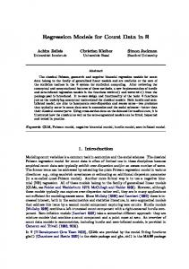
where d1 = k1 + 1 = 8 is a multiple of the frequency ratio m1 = 4, whereas d2 = k2 + 1 = 17 is not a multiple of m2 = 12. Here q1 = 2, q2 = 3 with parameterizations γ 1 = (1, −0.5)> , γ 2 = (2, 0.5, −0.1)> , which yield the shapes of functional constraints as plotted in Figure 2. The following R code produces a series according to the DGP characterized above: R> R> R> R> R> R> R> R> +

set.seed(1001) n set_x set_z expand_weights_lags(weights = c("nealmon", "nbeta"), from = 1, + to = c(2, 3), m = 1, start = list(nealmon = c(1, -1), + nbeta = rep(0.5, 3)))


1 2 3 4

23

weights lags starts nealmon 1:2 c(1, -1) nealmon 1:3 c(1, -1) nbeta 1:2 c(0.5, 0.5, 0.5) nbeta 1:3 c(0.5, 0.5, 0.5)

Given the sets of potential specifications for each variable as defined above, the estimation of all the models is performed by R> eqs_ic eqs_ic$candlist[[5]] eqs_ic modsel(eqs_ic, IC = "AIC", type = "restricted") which also prints the usual summary statistics as well as the testing of adequacy of the applied functional restriction using, by default, hAh_test. A word of caution is needed here to remind that, as is typical, the empirical size of a test corresponding to a complex model-selection procedure might not correspond directly to a nominal one of a single-step estimation.

3.6. Forecasting Conditional forecasting (with prediction intervals, etc.) using unrestricted U-MIDAS regression models which are estimated using lm can be performed using standard R functions, e.g.,

24


the predict method for ‘lm’ objects. Conditional point prediction given a specific model is also possible relying on a standard predict function. The predict method implemented in package midasr works similarly to the predict method for ‘lm’ objects. It takes the new data, transforms it into an appropriate matrix and multiplies it with the coefficients. Suppose we want to produce the forecast yˆT +1|T for model (12). To produce this forecast we need the data x4(T +1) , . . . , x4T −3 and z12(T +1) , . . . , z12T −4 . It would be tedious to calculate precisely the required data each time we want to perform a forecasting exercise. To alleviate this problem package midasr provides the function forecast. This function assumes that the model was estimated with the data up to low frequency index T. It is then assumed that the new data is the data after the low frequency T and then calculates the appropriate forecast. For example suppose that we have new data for one low frequency period for model (12). Here is how the forecast for one period would look like: R> newx newz forecast(eq_rb, newdata = list(x = newx, z = newz, trend = 251)) Point Forecast 1 28.28557 It is also common to estimate models which do not require new data for forecasting yt+` = 2 + 0.1t +

7 X (1)

16 X (2)

j=0

j=0

βj x4t−j +

βj z12t−j + εt+` ,

where ` is the desired forecasting horizon. This model can be rewritten as yt = 2 + 0.1(t − `) +

7+4` X j=4`

(1)

βj x4t−j +

16+12` X

(2)

βj z12t−j + εt ,

j=12`

and can be estimated using midas_r. For such a model we can get forecasts yˆT +`|T , . . . , yˆT +1|T using the explanatory variable data up to low frequency index T. To obtain these forecasts using the function forecast we need to supply NA values for explanatory variables. An example for ` = 1 is as follows: R> eq_f forecast(eq_f, newdata = list(x = rep(NA, 4), z = rep(NA, 12), + trend = 251)) Point Forecast 1 27.20452 Note that we still need to specify a value for the trend. In addition, the package midasr provides a general flexible environment for out-of-sample prediction, forecast combination, and evaluation of restricted MIDAS regression models using


25

the function select_and_forecast. If exact models were known for different forecasting horizons, it can also be used just to report various in- and out-of-sample prediction characteristics of the models. In the general case, it also performs an automatic selection of the best models for each forecasting horizon from a set of potential specifications defined by all combinations of functional restrictions and lag orders to be considered, and produces forecast combinations according to a specified forecast weighting scheme. In general, the definition of potential models in the function select_and_forecast is similar to that one used in the model selection analysis described in the previous section. However, different best performing specifications are most likely related with each low-frequency forecasting horizon ` = 0, 1, 2, . . . . Therefore the set of potential models (parameter restriction functions and lag orders) to be considered for each horizon needs to be defined. Suppose that, as in the previous examples, we have variables x and z with frequency ratios m1 = 4 and m2 = 12, respectively. Suppose that we intend to consider forecasting of y up to three low-frequency periods ` ∈ {1, 2, 3} ahead. It should be noted that, in terms of highfrequency periods, they correspond to `m1 ∈ {4, 8, 12} for variable x, and `m2 ∈ {12, 24, 36} for variable z. Thus these variable-specific vectors define the lowest lags6 of high-frequency period to be considered for each variable in the respective forecasting model (option from in the function select_and_forecast). Suppose further that in all the models we want to consider specifications having not less than 10 high-frequency lags and not more than 15 for each variable. This defines the maximum high-frequency lag of all potential models considered for each low-frequency horizon period ` ∈ {1, 2, 3}. Hence, for each variable, three corresponding pairs (`m1 + 10, `m1 + 15), ` ∈ {1, 2, 3} will define the upper bounds of ranges to be considered (option to in the function select_and_forecast). For instance, for variable x, three pairs (14, 19), (18, 23), and (22, 27) correspond to ` = 1, 2, and 3 and together with that defined in option from (see x = (4, 8, 12)) imply that the following ranges of potential models will be under consideration for variable x: • ` = 1 : from [4 − 14] to [4 − 19], • ` = 2 : from [8 − 18] to [8 − 23], • ` = 3 : from [12 − 22] to [12 − 27]. The other options of the function select_and_forecast are options of functions midas_r_ic_table, modsel and average_forecast. R> cbfc cbfc$accuracy$individual R> cbfc$accuracy$average report, respectively: • the best forecasting equations (in terms of a specified criterion out of the above-defined potential specifications), and their in- and out-of-sample forecasting precision measures for each forecasting horizon; • the out-of-sample precision of forecast combinations for each forecasting horizon. The above example illustrated a general usage of the function select_and_forecast including selection of best models. Now suppose that a user is only interested in evaluating a one step ahead forecasting performance of a given model. Suppose further that he/she a priori knows that the best specifications to be used for this forecasting horizon ` = 1 is with • mls(x, 4:12, 4, nealmon) with parameters x = c(2, 10, 1, -0.1) (the first one representing an impact parameter and the last three being the parameters of the normalized weighting function), and • mls(z, 12:20, 12, nealmon) with parameters z = c(-1, 2, -0.1), i.e., with one parameter less in the weighting function. Given already preselected and evaluated models, a user can use the function average_forecast to evaluate the forecasting performance. To use this function at first it is necessary to fit the model and then pass it to function average_forecast specifying the in-sample and outof-sample data, accuracy measures and weighting scheme in a similar manner to function select_and_forecast R> mod1 avgf R> R> R> R> R> R> R>

data("USqgdp", package = "midasr") data("USpayems", package = "midasr") y R> + R>

fulldata + R> + + R> R> R>

tb